Non-Gaussianity and the recovery of the mass power spectrum from the Ly$\alpha$ forest

Abstract

We investigate the effect of non-Gaussianity on the reconstruction of the initial mass field from the Ly$\alpha$ forest. We show that the transmitted flux of QSO absorption spectra are highly non-Gaussian in terms of the statistics, the kurtosis spectrum and scale-scale correlation. These non-Gaussianities can not be completely removed by the conventional algorithm of Gaussianization, and the scale-scale correlations are largely retained in the mass field recovered by the Gaussian mapping. Therefore, the mass power spectrum recovered by the conventional algorithm is systematically lower than the initial mass spectrum on scales at which the local scale-scale correlation is substantial. To reduce the non-Gaussian contamination, we present two methods. The first is to perform the Gaussianization scale-by-scale using the discrete wavelet transform (DWT) decomposition. We show that the non-Gaussian features of the Ly$\alpha$ forest basically will no longer exist in the scale-by-scale Gaussianized mass field. The second method is to choose a proper orthonormal basis (representation) to suppress the effect of the non-Gaussian correlations. In the quasilinear regime of cosmic structure formation, the DWT power spectrum is efficient for suppressing the non-Gaussian contamination. These two methods significantly improve the recovery of the mass power spectrum from the Ly$\alpha$ forest.

1 Introduction

Since high resolution QSO spectra became available, the transmitted flux in QSO spectra, or the Ly$\alpha$ forest, offers an unprecedented opportunity to study the large-scale structure of the universe and its evolution at redshifts beyond the galaxy redshift catalog (e.g. Bi & Davidsen 1997 and references within). A basic goal of this study is to reconstruct the initial mass field. Assuming that these objects trace the underlying matter field in some way, it seems to be possible to trace the evolution of mass field back in time. Because the initial mass field is expected to be Gaussian in many models of the origin of fluctuations, reconstructing the initial mass fluctuations is synonymous with recovering the mass power spectrum (e.g. Croft et al. 1999.)

The recovery of power spectrum from the Ly$\alpha$ forests relies upon two theoretical conjectures. The first is to assume that the transmitted flux of a QSO Ly$\alpha$ absorption spectrum is a point-to-point tracer of the underlying dark matter distribution. The Ly$\alpha$ forest has been successfully modeled by the absorption of the ionized intergalactic gas, of which the distribution is continuous, and locally determined by the underlying dark matter distribution (Bi 1993; Fang et al. 1993; Bi, Ge & Fang 1995; Hernquist et al 1996; Bi & Davidsen 1997; Hui, Gnedin & Zhang 1997). Thus, the transmitted flux of a QSO absorption spectrum at a given redshift depends only on the mass density of dark matter at the position corresponding to the redshift.

The second assumption is that the initial mass field can be recovered from the flux of QSO spectrum by the Gaussianization algorithm (Weinberg 1992; Croft et al. 1998). With this method, the shape of 1-D initial Gaussian density field with an arbitrary normalization can be recovered approximately from the observed flux by a point-to-point Gaussian mapping if the relation between flux and mass density is monotonous, i.e. the higher the underlying mass density, the stronger the Ly$\alpha$ absorption. The monotony would be a good approximation in the weak nonlinear or quasilinear evolutionary regime of the cosmic clustering.

This paper is trying to study the influence of the non-Gaussianity of the Ly$\alpha$ forest on the recovery of the initial power spectrum. It is motivated by the recently systematic detection of non-Gaussianity of the Ly$\alpha$ forests. Despite it is well known that the two-point correlation function of the Ly$\alpha$ absorption lines is quite weak, the distribution of these lines does show non-Gaussian behavior. For instance, it has been well known about ten years ago that the distribution of the nearest neighbor Ly$\alpha$ line intervals is different from a Poisson process (Duncan, Ostriker, & Bajtlik 1989; Liu and Jones 1990; Fang, 1991). Recently, the detection of the spectrum of higher order cumulants (Pando & Fang 1998a) and the scale-scale correlations (Pando et al. 1998) of the Ly$\alpha$ forests implies systematic non-Gaussianity on scales as large as about 10 h^-1 Mpc. The abundance of the Ly$\alpha$ line “clusters” identified with respect to the richness is also found to be significantly different from a Gaussian process (Pando & Fang 1996.)

According to the philosophy of the Gaussianization reconstruction, all the non-Gaussian features of the Ly$\alpha$ forests are not initial. It should be removed by the Gaussianization of the flux of QSO spectra. The recovered mass field should be Gaussian. The algorithm of Gaussian mapping is designed for removing the non-Gaussianities of the flux, and recovering a Gaussian mass field.

The idea of Gaussianization is exquisite. However, we will show that even though the current algorithm of Gaussian mapping does map the distribution of the flux value into a Gaussian probability distribution function (PDF), the above-mentioned non-Gaussianities of the Ly$\alpha$ forests still remain largely in the Gaussianized flux. Namely, the recovered field is not linear and Gaussian, but contaminated by the non-Gaussian behavior in the Ly$\alpha$ forest.

It has been recognized that the estimation of power spectrum is significantly affected by the non-Gaussian behavior, such as the correlation between band-averaged power spectra which is essentially the scale-scale correlation (e.g. Meiksin & White 1999). Therefore, with the current algorithm of Gaussianization, the recovered power spectrum is distorted by the non-Gaussianity of the Ly$\alpha$ forests. The question is then raised: how to improve the algorithm of Gaussianization in order to recover a mass field exempted from the non-Gaussianity of the Ly$\alpha$ forest? Or how to suppress the effect of the non-Gaussian contamination in estimation of the power spectrum? We try to investigate these problems in this paper.

This paper is organized as follows. In §2, using popular cold dark matter models, we present the non-Gaussian features in the transmitted flux of the Ly$\alpha$ forests. In §3, we demonstrate that the non-Gaussianity of mass field recovered by the conventional Gaussianization algorithm is about the same order as the original non-Gaussianity. Two alternatives which yield better Gaussianization are then proposed. In §4, the distortion of power spectrum by the non-Gaussianity is shown, and a possible way of suppressing the non-Gaussian effect on the power spectrum detection, i.e. properly choosing representation of the power spectrum, is suggested. We conclude this paper with a discussion of our findings in §5.

2 The Non-Gaussian features of the Ly$\alpha$ forests

2.1 Samples of the Ly$\alpha$ forests

To investigate the recovery method of mass power spectrum, we generate the simulation samples of the Ly$\alpha$ forest in the semi-analytic model of the intergalactic medium (IGM) developed by H.G. Bi et al. (Bi 1993; Fang et al. 1993; Bi, Ge & Fang 1995; Bi & Davidsen 1997.) This model can approximately fit most observed features of the Ly$\alpha$ forest, including the column density distribution and the number density of the Ly$\alpha$ forest lines; the distribution of the equivalent widths and their redshift dependence; the clustering and the Gunn-Peterson effect. Moreover, in this model, the relations among the dark matter field, the flux of the Ly$\alpha$ absorption and the power spectrum of reconstructed initial mass fields are under control. It would be very useful to reveal the problems of the reconstruction.

The model was described in detail in the above listed references. We now give a brief account of, especially, the fundamental physics underlying in this model. The basic assumption of the model is that the density distribution of the baryonic diffuse matter $n({\bf x})$ in the universe is determined by the underlying dark matter density distribution via a lognormal relation as

$$n({\bf x})=n_{0}\exp\left[\delta_{0}({\bf x})-\frac{<\delta_{0}^{2}>}{2}\right],$$ (1)

where $n_{0}$ is the mean number density, and $\delta_{0}({\bf x})$ is a Gaussian random field derived from the density contrast $\delta_{DM}$ of the dark matter by:

$$\delta_{0}({\bf x})=\frac{1}{4\pi x_{b}^{2}}\int\frac{\delta_{DM}({\bf x}_{1})}{|{\bf x}-{\bf x}_{1}|}e^{-\frac{|{\bf x}-{\bf x}_{1}|}{x_{b}}}d{\bf x}_{1}$$ (2)

in the comoving space, or

$$\delta_{0}({\bf k})=\frac{\delta_{DM}({\bf k})}{1+x_{b}^{2}k^{2}}$$ (3)

in the Fourier space. To take into account the effect of redshift distortion, the peculiar velocity field along the line of sight is also calculated by the simulation model (Bi 1993; Fang et al. 1993; Bi& Davidsen 1997.)

The Gaussian field $\delta_{DM}$ is produced in a cold dark matter model. To account for the baryonic effect on the transfer function, we adopt the fitting formula for power spectrum presented by Eisenstein & Hu (1999). Because the goal of this paper is mainly on examining the recovery method of power spectrum, we will not take into account the variants of CDM family, but only the “standard” one, i.e. the flat model ($\Omega_{0}=1.0$) normalized by the 4-year COBE data, and the $\Gamma=\Omega_{0}h$ is taken to be 0.3, where $h$ denotes the normalized Hubble parameter, and $\Omega_{0}$ is the cosmological density parameter of total mass. This model is compatible with the galaxy correlation observed on scales of $\sim 10$ h^-1 Mpc (Efstathiou et.al. 1992). The baryonic fraction in the total mass was fixed by the constraint from the primordial nucleosynthesis of $\Omega_{b}=0.0125$ h^-2 (Walker et.al, 1991).

The factor $x_{b}$ in Eq. (2) is the Jeans length of IGM given by

$$x_{b}\equiv\frac{1}{2\pi H_{0}}\left[\frac{2\gamma kT_{m}}{3\mu m_{p}\Omega(1+z)}\right]^{\frac{1}{2}},$$ (4)

where $T_{m}$ and $\mu$ are the density-average temperature and molecular weight of the IGM respectively, and $\gamma$ is the ratio of specific heats. The thermal equation of state of IGM is assumed to be polytropic, $T\propto n^{\gamma-1}$ with $\gamma=4/3$.

The lognormal relation, Eq.(1), has the following property: (1) When fluctuations are small, i.e. $(n/n_{0}-1)\simeq\delta_{0}$, Eq. (1) is just the expected linear evolution of the IGM; (2) On small scales as $|{\bf x}-{\bf x}_{1}|\ll x_{b}$, Eq. (1) becomes the well-known isothermal hydrostatic solution, which describes highly clumped structures such as intracluster gas, $n\propto\exp(-\mu m_{p}\psi_{DM}/\gamma kT)$, where $\psi_{DM}$ is the dark matter potential (Sarazin & Bahcall 1977).

The absorption optical depth at observed wavelength $\lambda$ is

$$\tau(\lambda)=\int^{t_{0}}_{t_{qso}}\sigma\left(\frac{c}{\lambda_{\alpha}}\frac{1+z}{1+z_{0}}\right)n_{HI}(t)dt,$$ (5)

where $z_{0}=(\lambda/\lambda_{\alpha})-1$, $t_{0}$ denotes the present time, $t_{qso}$ is the time corresponding to the redshift $z_{qso}$ of the QSO, and so does for the relation between $t$ and $z$; $\sigma$ is the absorption cross section at the Ly$\alpha$ transition, and $\lambda_{\alpha}=1216\AA$ represents the Ly$\alpha$ wavelength. The density of the neutral hydrogen atoms, $n_{HI}$, can be found from $n$ by the cosmic abundance of hydrogen, and photoionization equilibrium (Bi, Ge & Fang 1995.)

Obviously in this model, the relation between the transmitted flux, $F(\lambda)=e^{-\tau}$, and $n({\bf x})$ or $\delta_{0}({\bf x})$ is basically local. The non-locality is only caused by the width of the absorption cross section $\sigma$, and the peculiar velocity of the neutral hydrogen. Therefore, $F$ is approximately a point-to-point tracer of mass fluctuation $\delta_{0}({\bf x})$. Moreover, the $F$ is monotonically related to $\delta_{0}$, and then, to the density contrast $\delta_{DM}$ on scales larger than $x_{b}$.

In this paper, we produce the simulation samples in the redshift range $z=2.066\sim 2.436$ with $2^{14}$ pixels. The corresponding simulation size in the CDM model is 189.84 h^-1Mpc in comoving space which is long enough to incorporate most of the fluctuation power. The selection of this redshift range is to compare the simulation with the Keck spectrum of HS1700+64. The spectrum of HS1700+64 ranges from 3723.012Åto 5523.554Åwith the resolution $3$ kms^-1, or totally 55882 pixels in which the first $2^{14}$ pixels are chosen here. These data have been used for testing the model considered in Bi & Davidsen (1997).

2.2 The skewness and kurtosis spectra of the transmitted flux

If appropriate parameters of the intergalactic UV background are adopted, the lognormal IGM model described in §2.1 could explain successfully many observed properties of the Ly$\alpha$ forest and their evolution from redshift 2 to 4. Now we show that it also works against tests of the non-Gaussian features.

We use the wavelet transform to analyze the non-Gaussian behavior of the transmitted flux $F$. As a 1-D field, the flux $F(\lambda)$ in the wavelength range of $L=\lambda_{max}-\lambda_{min}$ is subject to a discrete wavelet transform (DWT) as

$$F=\bar{F}+\sum_{j=0}^{\infty}\sum_{l=0}^{2^{j}-1}\tilde{\epsilon}_{j,l}\psi_{j,l}(\lambda)$$ (6)

where $\psi_{j,l}(x)$, $j=0,1,...$, $l=0...2^{j}-1$, is an orthogonal and complete set of the DWT basis (the details of the DWT, see e.g. Fang & Thews 1998). The wavelet basis $\psi_{j,l}(x)$ is localized both in the physical space and the Fourier (scale) space. The function $\psi_{j,l}(x)$ is centered at position $lL/2^{j}$ of the physical space, and at wavenumber $2\pi\times 2^{j}/L$ of the Fourier space. Therefore, the wavelet function coefficients (WFCs), $\tilde{\epsilon}_{j,l}$, have two subscripts $j$ and $l$. They describe the fluctuation of the flux on scale $L/2^{j}$ at position $lL/2^{j}$. To be more specific, we will use the Daubechies 4 wavelet in this paper, although all conclusions are not affected by this particular choice as long as a compactly supported wavelet basis is used.

The WFC, $\tilde{\epsilon}_{j,l}$, is computed by the inner product of

$$\tilde{\epsilon}_{j,l}=<F*\psi_{j,l}>.$$ (7)

Since the DWT bases are complete, the WFCs contain all information of the flux.

Note that the $\psi_{j,l}(x)$ are orthogonal with respect to the position index $l$, and therefore, for an ergodic field, the $2^{j}$ WFCs at a given $j$, i.e. $\tilde{\epsilon}_{j,l}$, $l=0,1...2^{j}-1$, can be treated as independent measures of the flux field. The $2^{j}$ WFCs, $\tilde{\epsilon}_{j,l}$, from one realization of $F(\lambda)$ can be employed as a statistical ensemble. In other words, when the fair sample hypothesis holds (Peebles 1980), an ensemble average can be estimated equivalently by averaging over $l$, i.e. $\langle\tilde{\epsilon}_{j,l}\rangle\simeq(1/2^{j})\sum_{l=0}^{2^{j}-1}\tilde{\epsilon}_{j,l}$, where $\langle...\rangle$ denotes the ensemble average. The distribution of $\tilde{\epsilon}_{j,l}$ represents approximately the one-point distribution of the WFCs at a given scale $j$.

The non-Gaussianity of the flux $F(\lambda)$ can be directly measured by the deviation of the one-point distribution from a Gaussian distribution. For this purpose, we calculate the cumulant moments defined by

$$I^{2}_{j}=M^{2}_{j},$$ (8)

$$I^{3}_{j}=M^{3}_{j},$$ (9)

$$I^{4}_{j}=M^{4}_{j}-3M^{2}_{j}M^{2}_{j},$$ (10)

$$I^{5}_{j}=M^{5}_{j}-10M^{3}_{j}M^{2}_{j},$$ (11)

where

$$M^{n}_{j}\equiv\frac{1}{2^{j}}\sum_{l=0}^{2^{j}-1}(\tilde{\epsilon}_{j,l}-\overline{\tilde{\epsilon}_{j,l}})^{n}.$$ (12)

The second order cumulant moment gives the DWT power spectrum (§4) (Pando & Fang 1998). For Gaussian fields all the cumulant moments higher than order 2 are zero. Thus one can measure the non-Gaussianity by $I^{n}_{j}$ with $n>2$. We call $I^{n}_{j}$ the DWT spectrum of $n$-th cumulant. The cumulant measures $I^{3}_{j}$ and $I^{4}_{j}$ are related to the well known skewness and kurtosis, respectively, defined by

$$S_{j}\equiv\frac{1}{(I_{j}^{2})^{3/2}}I^{3}_{j},$$ (13)

$$K_{j}\equiv\frac{1}{(I_{j}^{2})^{2}}I^{4}_{j}.$$ (14)

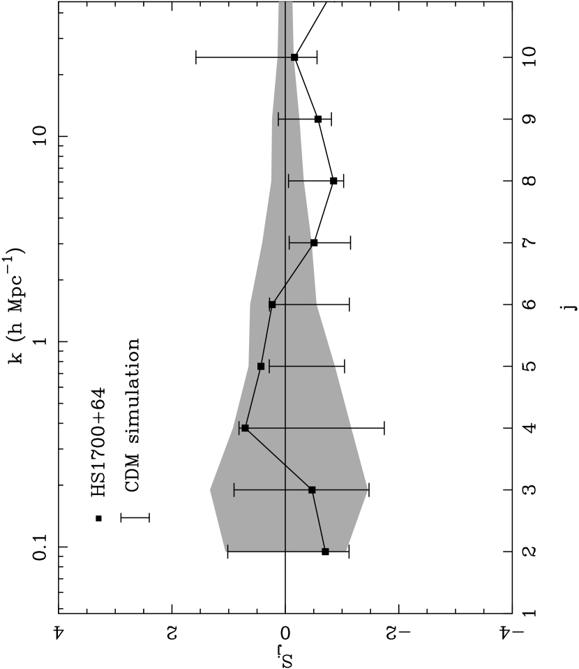
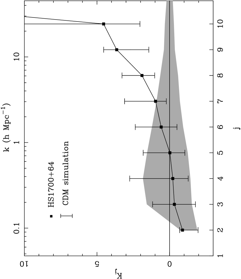
Using the skewness and kurtosis spectra as statistical indicators, a significant non-Gaussian behavior has been found in the distribution of Ly$\alpha$ forest lines (Pando & Fang 1998a). The skewness and kurtosis spectra of the transmitted flux in 100 simulated samples are shown in Figs. 1 and 2, respectively. To assess the statistical significance, the 95% confidence range from 100 realizations of Gaussian noise are also displayed in these figures. Clearly, the kurtosis spectrum of simulated $F$ shows difference from the Gaussian noise spectra on the scales $j\geq 8$ (or $\leq 1.5$ h^-1 Mpc) with 95% confidence. The skewness spectrum does not show significant difference from the Gaussian noise till $j=11$ ($\sim 100$ h^-1 kpc). These results are qualitatively consistent with that for the observed forest line distributions. In addition, the skewness and kurtosis spectra of the flux of HS1700+64 are also presented in Figs. 1 and 2. Obviously, the CDM model is in excellent agreement with the observation.

2.3 The scale-scale correlations of the transmitted flux

The scale-scale correlations measure the correlations between the fluctuations on different scales (Pando et al. 1998, Pando, Valls–Gabaud, & Fang 1998, Feng, Deng & Fang 2000). This non-Gaussianity is independent from the higher order cumulants (§2.2), which are only of $j$ dependent. A simplest measure of the scale-scale correlation is given by

$$C^{p,p}_{j}=\frac{2^{(j+1)}\sum_{l=0}^{2^{j+1}-1}\tilde{\epsilon}^{p}_{j;[l/2]}\;\tilde{\epsilon}^{p}_{j+1;l}}{\sum\tilde{\epsilon}^{p}_{j,[l/2]}\sum\tilde{\epsilon}^{p}_{j+1;l}}$$ (15)

where $p$ is an even integer, and [  ]’s denote the integer part of the quantity. Because $Ll/2^{j}=L2l/2^{j+1}$, the position $l$ at scale $j$ is the same as the positions $2l$ and $2l+1$ at scale $j+1$. Therefore, $C_{j}^{p,p}$ measures the correlation between fluctuations on scale $j$ and $j+1$ at the same physical point. For Gaussian fields, $C_{j}^{p,p}=1$. $C_{j}^{p,p}>1$ corresponds to the positive scale-scale correlation, and $C_{j}^{p,p}<1$ to the negative case. One variant of the above definition is

$$C^{p,p}_{j,\Delta l}=\frac{2^{(j+1)}\sum_{l=0}^{2^{j+1}-1}\tilde{\epsilon}^{p}_{j;[l/2]+\Delta l}\;\tilde{\epsilon}^{p}_{j+1;l}}{\sum\tilde{\epsilon}^{p}_{j,[l/2]}\sum\tilde{\epsilon}^{p}_{j+1;l}}.$$ (16)

This statistics is for measuring the correlations between fluctuations on scales $j$ and $j+1$, but at different positions, i.e. the fluctuation at scale $j$ is displaced from the $j+1$ fluctuation by a distance $\Delta lL/2^{j}$.

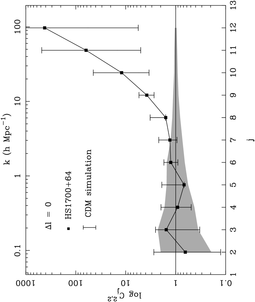
The scale-scale correlation $C_{j}^{2,2}$ calculated from the simulated transmitted flux and HS1700+64 are shown in Fig. 3. Clearly, the values of $C_{j}^{2,2}$ are significantly larger than unity and well above the Gaussian noise spectra on all the scales $j\geq 7$. This result is also qualitatively in agreement with the scale-scale correlation of the Ly$\alpha$ forests (Pando et al. 1998.). Figure 3 also indicates that the model of §2.1 is still in a good shape of fitting the observed non-Gaussian correlation.

Similar to Eq.(15) for the correlation between scales $|j-j^{\prime}|=1$, one may define, in principle, the correlation between two arbitrary scales with $|j-j^{\prime}|>1$. However, for hierarchical clustering the scale-scale correlation is quantified mainly by $|j-j^{\prime}|=1$. Therefore, we will not calculate the scale-scale correlations for $|j-j^{\prime}|>1$.

3 The Non-Gaussian features of the Gaussian-recovered mass fields

3.1 Non-Gaussianity after Gaussianization

The cosmological reconstruction is to extract the power spectrum of the initial linear mass fluctuations from the observed distribution of various tracers of the evolved density field. The algorithm of Gaussianization was designed for recovering the primordial density fluctuations from an observed galaxy distribution (Weinberg 1992). This method has been recently applied to recovering the linear density field and its power spectrum from the observed transmitted flux $F$ of QSO absorption spectra (Croft et al 1998, 1999).

The key step of the Gaussianization algorithm is a pixel-to-pixel mapping from an observed flux $F$ into the density contrast $\delta$. The probability distribution function (PDF) of the observed transmitted flux $F$ is generally non-Gaussian, while the PDF of the initial density contrasts $\delta\equiv(n/n_{0})-1$ is assumed to be Gaussian in large variety of galaxy formation models. The relation between $F=\exp(-\tau)$ and $\delta$ is monotonic, i.e. high initial density $\delta$ pixels evolved into high $\tau$ pixels, low initial density pixels into low $\tau$ pixels. Thus, using the observed $F$, one can sort out the total N pixels by the amount of $F$ in the ascending order: the pixel with lowest $F$ is labeled by 1st, the next higher $F$ pixel is labeled by 2nd, and so on. For the n-th pixel, we then assign the density contrast $\delta$, which is given by the solution of the equation $(2\pi)^{-1/2}\int_{-\infty}^{\delta}\exp(-x^{2}/2)dx=n/N$. Thus, the Gaussian mapping produces a mass field with the same rank order as the flux but with a Gaussian PDF of $\delta({\bf x})$. The overall amplitude of the recovered power spectrum should be determined by a separate procedure. For instance, we may set up the initial condition by using the recovered spectrum, evolve the simulation to the observed redshift and then normalize the spectrum by requiring that the simulation reproduces the observed power spectrum of the transmitted QSO flux. This amplitude normalization is model-dependent.

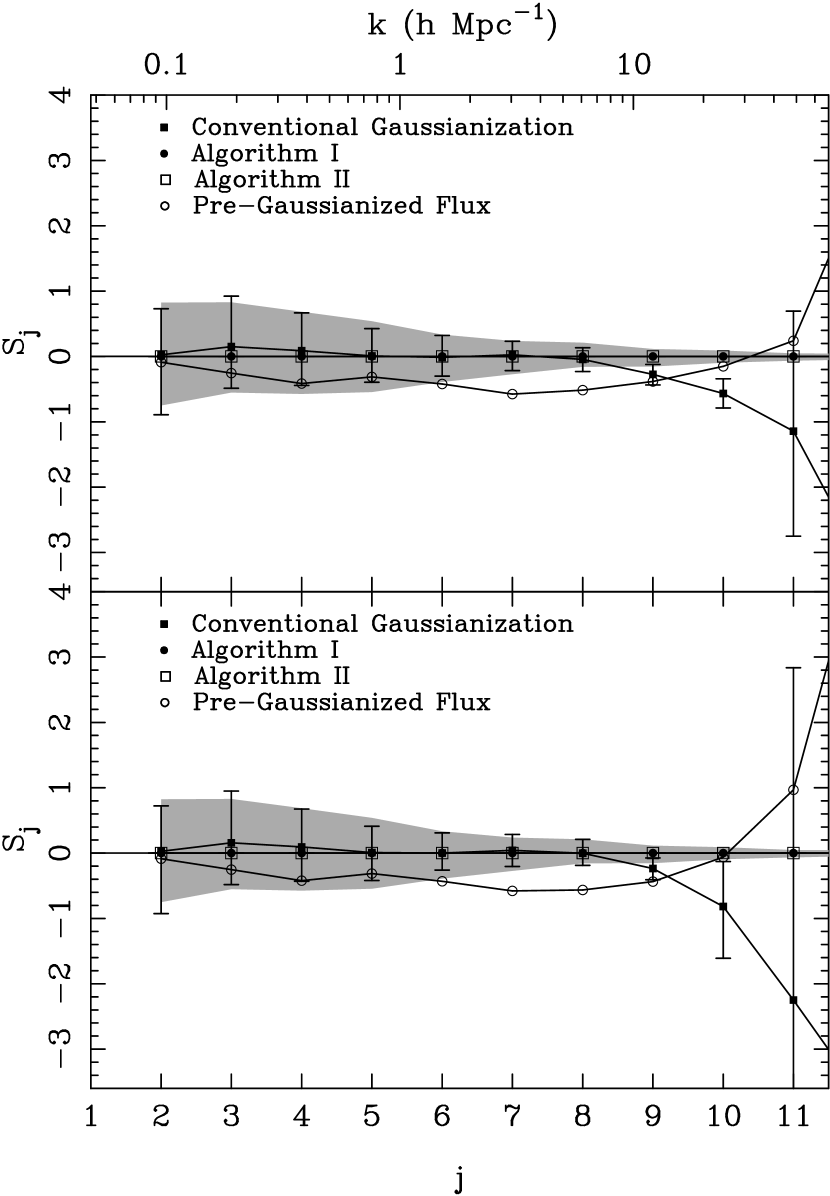
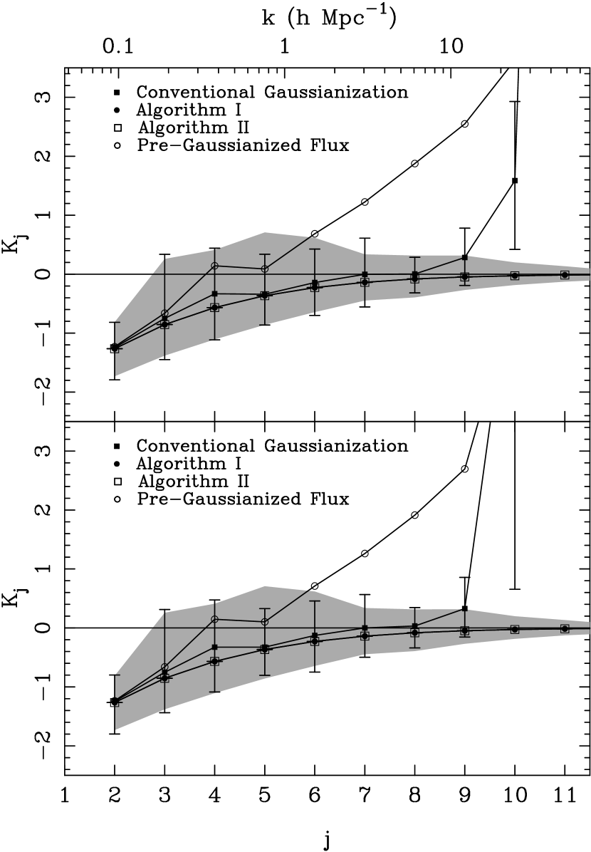
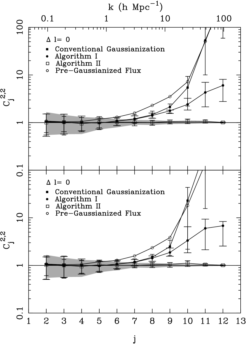
We apply the Gaussianization to 100 simulation samples of the QSO transmitted flux, and measure the skewness and kurtosis spectrum as well as the scale-scale correlation. The results are displayed in Figs. 4 - 6. For comparison, the non-Gaussian spectra of the flux in Figs. 1 - 3. are also plotted correspondingly. Figs. 4 - 6 show that the Gaussianized flux still largely exhibits non-Gaussian features. Especially, the scale-scale correlations of the Gaussianized field is as strong as the pre-Gaussianized flux on scales $j\geq 10$. That is, the recovered density field is seriously contaminated by the non-Gaussianities in the original flux.

3.2 The efficiency of the conventional Gaussianization

The reason for the lower efficiency of the conventional Gaussian mapping (§3.1) is simple. The initial Gaussian random mass field is assumed to be a superposition of independent modes, of which the PDFs are Gaussian. For instance, in the Fourier representation, all Fourier modes of a Gaussian mass field are Gaussian, i.e. they have Gaussian PDF of the amplitudes and randomized phases. The conventional algorithm considered only the Gaussianization of one variable, $\delta$. It does not guarantee the Gaussianization of the amplitudes and phases of all relevant modes. In other words, the Gaussian mapping algorithm will work perfectly for a system with one stochastic variable, but not so for a field.

Alternatively, this problem can also be seen via the DWT representation. Using eq.(1), any 1-D mass field given by density contrast $\delta(x)$ ($\bar{\delta}=0$) can be decomposed with respect to a DWT basis as

$$\delta(x)=\sum_{j=0}^{\infty}\sum_{l=0}^{2^{j}-1}\tilde{\epsilon}^{M}_{j,l}\psi_{j,l}(x),$$ (17)

where the superscript $M$ means mass. Equation (17) represents a linear superposition of modes $\psi_{j,l}$. As has been pointed out in §2.2, for a given $j$, the 2^j WFCs $\tilde{\epsilon}^{M}_{j,l}$ form a statistical ensemble. The distribution of the 2^j WFCs gives the one-point distribution of the amplitude of mode at the scale $j$. For the initial Gaussian mass field, these one-point distributions should be Gaussian. Obviously, the Gaussian PDF of $\delta$ does not imply that the one-point distributions of the WFCs for all $j$ are Gaussian (the central limit theorem). The amplitude $\delta$ can only play the role as one variable of the field.

Moreover, even when the one-point distributions of 2^j WFCs at all $j$ are Gaussianized, the mass field could still be non-Gaussian. For instance, suppose the one-point distribution of the 2^j WFCs, $\tilde{\epsilon}^{M}_{j,l}$, on scale $j$, is Gaussian. If the WFCs on scale $j+1$ is given by

$$\tilde{\epsilon}^{M}_{j+1;2l} = a\tilde{\epsilon}^{M}_{j,l},$$ (18)

$$\tilde{\epsilon}^{M}_{j+1;2l+1} = b\tilde{\epsilon}^{M}_{j,l},$$

where $a$ and $b$ are arbitrary constant, the one-point distribution of the 2^j+1 WFCs $\tilde{\epsilon}^{M}_{j+1,l}$ is also Gaussian. However, Eq.(18) leads to a strong correlation between $\tilde{\epsilon}^{M}_{j+1,l}$ and $\tilde{\epsilon}^{M}_{j,l}$. This is an example of the scale-scale correlation, i.e. the scale $j+1$ fluctuations are always proportional to those on the scale $j$ at the same position. Moreover, this correlation can not be eliminated by the Gaussianization of $\tilde{\epsilon}^{M}_{j;l}$. The Gaussian mapping changes all the WFCs at a given position (pixel) by a same amplifying or reducing factor, and therefore, the local relations Eq.(18) remains.

The scale-scale correlations only depend upon the statistical behavior of the fluctuation distribution with respect to the index $j$. Therefore, a Gaussian field requires the uncorrelation between the distributions of WFCs with different $j$. This uncorrelation corresponds to decorrelating the band average Fourier modes, which will be discussed in detail in §4.

3.3 Algorithms of scale-by-scale Gaussianization

Based on the considerations in the last section, we may design an algorithm which is capable of reducing the contamination of the non-Gaussianity, and produce fields with less non-Gaussianity.

The new method is based on the scale-by-scale decomposition of flux and mass field. From Eq.(6), we have

$$F=F^{j}+\sum_{j^{\prime}=j}^{\infty}\sum_{l=0}^{2^{j^{\prime}}-1}\tilde{\epsilon}_{j^{\prime},l}\psi_{j^{\prime},l},$$ (19)

and

$$F^{j}\equiv\bar{F}+\sum_{j^{\prime}=0}^{j-1}\sum_{l=0}^{2^{j^{\prime}}-1}\tilde{\epsilon}_{j^{\prime},l}\psi_{j^{\prime},l}.$$ (20)

$F^{j}$ is actually a smoothed $F$ by a filter on the scale $j$. There is a recursion relation in $F^{j}$ given by

$$F^{j+1}=F^{j}+\sum_{l=0}^{2^{j}-1}\tilde{\epsilon}_{j,l}\psi_{j,l}.$$ (21)

Namely, flux $F^{j+1}$ can be reconstructed from flux $F^{j}$ and 2^j WFCs $\tilde{\epsilon}_{j,l}$ at the scale $j$. Similarly, for a mass distribution, we have

$$\delta=\delta^{j}+\sum_{j^{\prime}=j}^{\infty}\sum_{l=0}^{2^{j^{\prime}}-1}\tilde{\epsilon}^{M}_{j^{\prime},l}\psi_{j^{\prime},l},$$ (22)

$$\delta^{j}\equiv\sum_{j^{\prime}=0}^{j+1}\sum_{l=0}^{2^{j^{\prime}}-1}\tilde{\epsilon}^{M}_{j^{\prime},l}\psi_{j^{\prime},l},$$ (23)

and

$$\delta^{j+1}=\delta^{j}+\sum_{l=0}^{2^{j}-1}\tilde{\epsilon}^{M}_{j,l}\psi_{j,l}.$$ (24)

Since the relations between $F$ and $\delta$ are local and monotonic, the smoothed flux $F^{j+1}$ depends only on the smoothed mass field $\delta^{j+1}$, and one can perform a local and monotonic mapping between $F^{j+1}$ and $\delta^{j+1}$. Thus, we can implement the reconstruction of the mass field $\delta^{j+1}$ from $F^{j+1}$ by a scale-by-scale Gaussianization algorithm (hereafter referred to as algorithm I):

1. Supposing the reconstruction down to the scale $j$ has been done, i.e. the $\delta^{j}$ is known already;

2. Calculating the WFCs of the flux $F$ on the scale $j$;

3. Making the Gaussian mapping of the 2^j WFCs $\tilde{\epsilon}_{j,l}$, and assigning the Gaussianized result, $\varepsilon_{j,l}$, to the 2^j pixels according to the rank order. The distribution of $\varepsilon_{j,l}$ is Gaussian with zero mean and variance one.

4. Finding the 2^j WFCs of mass field by

$$\tilde{\epsilon}^{M}_{j,l}=\nu\varepsilon_{j,l}.$$ (25)

where the parameter $\nu$ is a normalization factor to be determined. The one-point distribution of the WFCs of mass field at the scale $j$, $\tilde{\epsilon}^{M}_{j,l}$, is then Gaussianized.

5. Reconstructing the mass field $\delta^{j+1}$ on scale $j+1$ by the recursion relation Eq.(24)

6. To determine the parameter $\nu$, we require that the DWT power spectrum of the flux $F^{j+1}$ simulated from $\delta^{j+1}$ reproduces the observed flux $F^{j+1}$. We have then $\delta^{j+1}$. The reconstruction of mass field on the scale $j+1$ is done.

Repeating the steps 1 to 6, one can reconstruct the mass field on scales from large to small until the scale of the resolution of the flux $F$, or the scale on which the relation between $F$ and $\delta$ is no longer local.

Figure 7 illustrates the transmitted flux, the initial density field and the recovered density field by algorithm I. The recovered 1D density field is in excellent agreement with the original density field scale-by-scale. The non-Gaussianities of the recovered fields by algorithm I are shown in Figs. 4 - 6. The skewness and kurtosis spectra exhibit almost nothing but Gaussianity. The scale-scale correlation is also significantly reduced.

The Gaussianization algorithm I is conceptually clear. However, it needs to determine the normalization factor $\nu$ at each scale. Therefore, it is rather cumbersome to do the numerical calculation. Moreover, there is still somewhat residual scale-scale correlation in the recovered mass field. In fact, algorithm I does ensure the Gaussian PDF of $\tilde{\epsilon}^{M}_{j,l}$, but it is unable to remove all the correlation between different modes, just as the simple example [Eq.(18)] demonstrated in §3.2.

To avoid the multiple normalizations and keep the virtues of scale-by-scale Gaussianization, we design an alternative algorithm as follows (hereafter referred to as algorithm II):

1. Using the conventional Gaussianization (§3.1) to reconstruct the mass field, i.e. to perform Gaussian mapping of the density contract $\delta$ and normalize the mass field by requiring that the evolved simulations reproduce the power spectrum of the observed flux.

2. Calculating the WFCs $\tilde{\epsilon}_{j,l}$ of the recovered mass field $\delta^{M}$ on each scale $j$.

3. Similar to the step 3 of algorithm I, making the Gaussianization of $\tilde{\epsilon}_{j,l}$ for each scale $j$ to produce unnormalized WFCs $\varepsilon^{M}_{j,l}$.

4. Normalizing the WFCs $\varepsilon^{M}_{j,l}$ on scale $j$ by requiring that the variance of $\varepsilon^{M}_{j,l}$, i.e., the 2nd cumulant moment $I_{j}^{2}$ [Eq.(7)], is the same as those for the WFCs $\tilde{\epsilon}_{j,l}$.

5. For each scale $j$, randomizing the spatial sequence of the Gaussianized WFCs $\varepsilon^{M}_{j,l}$, i.e., making a random permutation among the index $l$.

6. Using these WFCs $\varepsilon^{M}_{j,l}$, one can reconstruct the mass density field by Eq.(24) till the scale given by the resolution of the flux.

Algorithm II is still scale-by-scale in nature. However, the normalization is one only once for the recovered $\delta$. The step 4 ensure that the normalization is unchanged after the step 3, which eliminates the non-Gaussianities of the skewness and kurtosis spectra. Step 5 is for eliminating the residual scale-scale correlations by a randomization of the spatial index $l$ of $\tilde{\epsilon}_{j,l}$. Namely, it changes only the position of $\tilde{\epsilon}_{j,l}$, but not the values. Therefore, it is similar to a randomization of phases of the Fourier modes, and will not change the normalization of the amplitude and power spectrum of the fields.

Figs. 4 - 6 show that the Gaussianized field by the algorithm II contains almost none of the non-Gaussian features considered. However, it should be pointed out that the field given by algorithm II is no longer a point-to-point reconstruction due to the randomization of $l$. Namely, the recovered field will not be point-to-point the same as the field shown in Fig. 7. Nonetheless, since the purpose of the Gaussianization is to recover the power spectrum of the primordial density fluctuations, algorithm II is a valuable approach. As will be shown in next section, the algorithm II gives more unbiased estimation of power spectrum by the standard FFT technique.

In order to illustrate the effect of the peculiar velocities on the Gaussianization, each of Figs. 4 - 6 contains two panels: one employed the simulation samples including the effects of peculiar velocities, and the other did not. All the figures show that for the algorithm I, the effect of peculiar velocities is significant only on small scales $j>9$, or $k>10$ h Mpc^-1; while for algorithm II, the effect of peculiar velocities appears on smaller scales. Therefore, our proposed scale-by-scale Gaussianization methods would not be affected by the peculiar velocities as least up to the scale j=9.

4 Recovery of mass power spectrum from the transmitted QSO flux

4.1 The power spectrum in different representations

As a preparation for measuring the non-Gaussian effects on power spectrum recovery, we first discuss the representation of power spectrum. Principally, a random field can be described by any complete orthonormal basis (representation). Although the default usage of power spectrum is defined on the Fourier basis, one can define the power spectrum with respect to different representation. This is due to the fact that the Parseval’s theorem holds for any complete and orthonormal basis decomposition.

In the Fourier representation, the power spectrum of a 1-D density field $\delta(x)$ is given by

$$P(n)=|\hat{\delta}_{n}|^{2}.$$ (26)

where $\hat{\delta}_{n}$ is the Fourier transform of $\delta(x)$. $|\hat{\delta}_{n}|^{2}$ measures the power of mode $n$ because of Parseval’s theorem

$$\frac{1}{L}\int_{0}^{L}\delta^{2}(x)dx=\sum_{n=-\infty}^{\infty}|\hat{\delta}_{n}|^{2}.$$ (27)

Similarly, we have the Parseval’s theorem for the DWT transform given by (Fang & Thews 1998, Pando & Fang, 1998b)

$$\frac{1}{L}\int_{0}^{L}\delta^{2}(x)dx=\sum_{j=0}^{\infty}\frac{1}{L}\sum_{l=0}^{2^{j}-1}\tilde{\epsilon}^{2}_{j,l}.$$ (28)

(For simplicity, we ignore the superscript $M$ on $\tilde{\epsilon}_{j,l}$). Therefore, the term $\tilde{\epsilon}^{2}_{j,l}$ describes the power of mode $(j,l)$, and the total power on the scale $j$ is

$$P_{j}=\frac{1}{L}\sum_{l=0}^{2^{j}-1}|\tilde{\epsilon}_{j,l}|^{2},$$ (29)

which defines the DWT power spectra $P_{j}$.

Generally, the second order correlation functions of $\hat{\delta}_{n}$ or $\tilde{\epsilon}_{j,l}$ can be converted from each other by

$$\langle\tilde{\epsilon}_{j,l}\tilde{\epsilon}_{j^{\prime},l^{\prime}}\rangle=\sum_{n,n^{\prime}=-\infty}^{+\infty}\langle\hat{\delta}_{n}\hat{\delta}^{*}_{n^{\prime}}\rangle\hat{\psi}_{j^{\prime},l^{\prime}}(n^{\prime})\hat{\psi}^{*}_{j,l}(n)$$ (30)

$$\langle\hat{\delta}_{n}\hat{\delta}^{*}_{n^{\prime}}\rangle=\sum_{j,j^{\prime}=0}^{+\infty}\sum_{l=0}^{2^{j}-1}\sum_{l^{\prime}=0}^{2^{j^{\prime}}-1}\langle\tilde{\epsilon}_{j,l}\tilde{\epsilon}_{j^{\prime},l^{\prime}}\rangle\hat{\psi}_{j,l}(n)\hat{\psi}^{*}_{j^{\prime},l^{\prime}}(n^{\prime})$$ (31)

where $\hat{\psi}_{j,l}(n)$ is the Fourier transform of $\psi_{j,l}(x)$. For an homogeneous random field, $\langle\hat{\delta}_{n}\hat{\delta}^{*}_{n^{\prime}}\rangle=\langle|\hat{\delta}_{n}|^{2}\rangle\delta_{n,n^{\prime}}$, we have then

$$\langle\tilde{\epsilon}^{2}_{j,l}\rangle=\sum_{n=-\infty}^{+\infty}\langle|\hat{\delta}_{n}|^{2}\rangle|\hat{\psi}_{j,l}(n)|^{2}$$ (32)

or

$$P_{j}=\sum_{n=-\infty}^{+\infty}P(n)|\hat{\psi}(n/2^{j})|^{2}$$ (33)

where $\hat{\psi}(n/2^{j})$ is the Fourier transform of the generating wavelet $\psi(x)$ (Pando & Fang 1998b). In Eq. (33) the function $|\hat{\psi}(n/2^{j})|^{2}$ plays the role of window function in the wavenumber $n$ space. The function $\hat{\psi}(n)$ is localized in $n$-space. For the Daubechies 4 wavelet, $|\hat{\psi}(n)|$ is peaked at $n=\pm n_{p}$ with the width of $\Delta n_{p}$. Therefore, the DWT spectrum $P_{j}$ gives an estimator of the “band averaged” Fourier power spectrum within the band centered at

$$\log n=(\log 2)j+\log n_{p},$$ (34)

with the band width,

$$\Delta\log n=\Delta n_{p}/n_{p}.$$ (35)

As the mean of the WFCs $\tilde{\epsilon}_{j,l}$ over $l$ is zero, so the second cumulant moment $I_{j}^{2}$ is related to DWT spectrum $P_{j}$ by $I_{j}^{2}=(L/2^{j})P_{j}$, we will use variance $I_{j}^{2}$ as the estimator of DWT power spectrum instead of $P_{j}$.

For a Gaussian field, the statistical behavior are completely determined by the second order statistics of the Gaussian variables $\hat{\delta}_{n}$ or $\tilde{\epsilon}_{j,l}$. Theoretically, the power spectrum estimators $P(n)$ and $P_{j}$ present the equivalent description. However, as will be shown below, once non-Gaussianity appears, these estimators will no longer be equivalent.

4.2 Effect of non-Gaussianity on the recovery of mass power spectrum

Using the 100 realizations of the mass density fields recovered by the conventional algorithm, and algorithm I and II of the Gaussianization, we calculated the power spectra by the standard FFT technique. To reveal the effect of non-Gaussianity on the power spectrum estimation, we do not include the effects of instrumental noise and continuum fitting in the synthetic spectra. The dominant sources of error in estimation of power spectrum would be the cosmic variance and the non-Gaussian effects.

Figure. 8 compares the power spectra obtained by different Gaussianization methods. The 1-D linear power spectrum of Eq.(3) is also shown by solid line. These power spectra are normalized to the present. In general, the recovered power spectrum can match the shape of the linear theory over a wide range of wavelength, especially on larger wavelength. Yet, the recovered spectra show somewhat systematic departure from the initial mass power spectrum with the increase of wavenumbers. For the conventional Gaussianization, the recovered power spectrum falls below the initial power spectrum on scales of $j\geq 8$ or $k\sim 1.5$ h^-1 Mpc. The power spectrum recovered by the algorithm I is better than the conventional Gaussianization, and the recovery by algorithm II gives the best one, which is almost the same as the initial power spectrum on all scales.

Comparing Fig. 8 with Figs. 4 - 6, we can see that the scales on which the depression of the recovered power spectrum appears is always the same as the scale on which the scale-scale correlations become significant. Moreover, the less the scale-scale correlation (Fig. 6), the less the depression. This indicates that the recovered spectrum is substantially affected by the non-Gaussianities, especially, the scale-scale correlations. Actually, this effect has already been recognized by Meiksin & White (1998) in analyzing N-body simulation samples. Namely, the goodness of a power spectrum estimation is significantly dependent on the correlation between the Fourier power spectra averaged at different scale bands.

Back to the definition of scale-scale correlation Eq. (15), and recall that the average over an ensemble is equivalent to the spatial average taken over one realization, Eq.(15) can be rewritten as

$$C_{j}^{2,2}=\frac{\langle\hat{P}_{j}\hat{P}_{j+1}\rangle}{\langle\hat{P}_{j}\rangle\langle\hat{P}_{j+1}\rangle}.$$ (36)

Hence, the scale-scale correlation is actually a measure of the correlation between the Fourier power spectra averaged at different scale bands. This can also be seen from Eq.(31) that the Fourier power spectrum around $n$ depends on the fluctuations on different $j$, and therefore, their non-Gaussian correlations.

Because the algorithm II is most effective for eliminating the scale-scale correlations, the resulting power spectrum shows the best recovery of the linear model.

4.3 Suppression of non-Gaussian correlations by representation

In the DWT representation, the power spectrum (29) does not depend on modes at the scales different from $j$, and therefore the scale-scale correlation will not affect the estimation of $P_{j}$. One can expect that the DWT spectrum estimator, $P_{j}$, will give a better recovery of the initial power spectrum.

Fig. 9 displays the DWT power spectrum $P_{j}$ for mass fields given by the different Gaussianization methods. The DWT power spectrum in the linear CDM model is also shown by solid line, which is calculated from the Fourier linear power spectrum by Eq. (33) in the continuous limit of $n$. This figure indicates that even for the mass field recovered from conventional Gaussianization, the DWT power spectrum is in good agreement with the initial DWT mass power spectrum up to the scale $j=9$. This is already much better than its counterpart in the Fourier representation, for which the power spectrum shows significant difference from the linear spectrum on scale $j\sim 8$. For the algorithm I and II, the DWT power spectrum also gives the good results. In addition, the errors due to the cosmic variance and normalization in the DWT spectrum are manifestly smaller than that of Fourier spectrum.

The DWT power spectrum $P_{j}$ (29) is given by the summation of $|\tilde{\epsilon}_{j,l}|^{2}$ over $l$ at a given scale. Therefore, the non-Gaussian effect on estimation of $P_{j}$ mainly arises from the correlation between the WFCs $\tilde{\epsilon}_{j,l}^{2}$ at different $l$, which can be measured by

$$Q^{2,2}_{j,\Delta l}=\frac{2^{j}\sum_{l=0}^{2^{j}-1}\tilde{\epsilon}^{2}_{j;l}\;\tilde{\epsilon}^{2}_{j;l+\Delta l}}{\sum\tilde{\epsilon}^{2}_{j,l}\sum\tilde{\epsilon}^{2}_{j;l+\Delta l}}.$$ (37)

$Q^{2,2}_{j,\Delta l}$ gives the correlation between the density fluctuations on the same scale $j$ at different places $l$ and $l+\Delta l$.

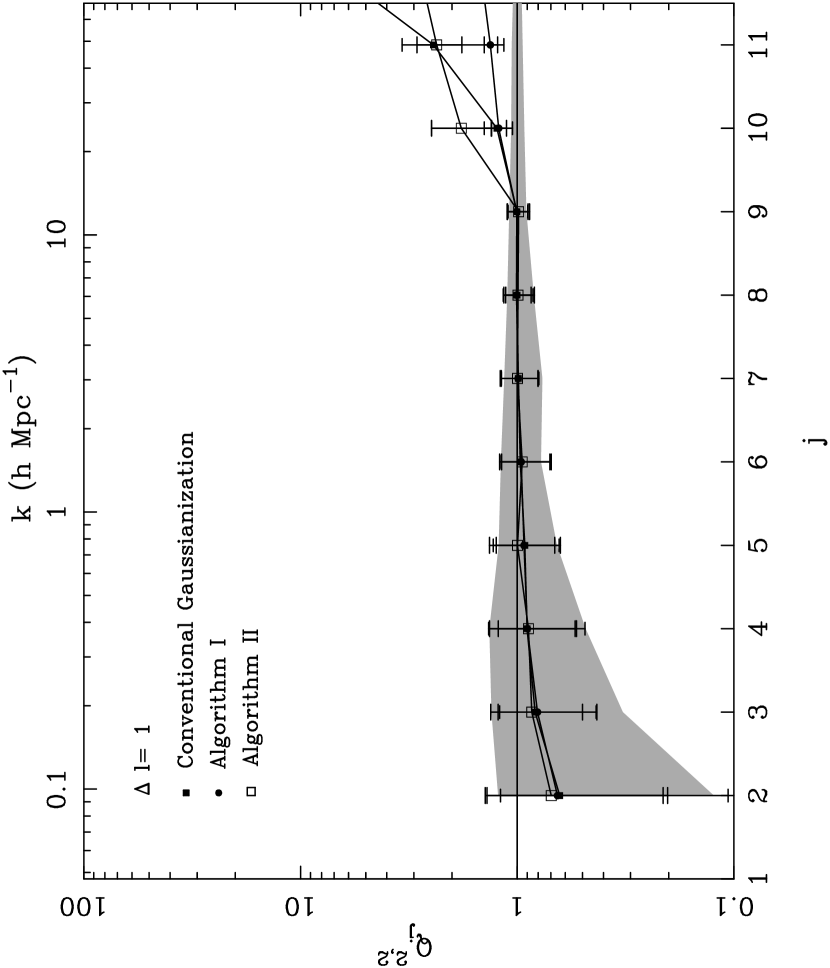
Fig. 10 displays the correlations $Q^{2,2}_{j,\Delta l}$ with $\Delta l=1$. It shows that this non-Gaussianity can be ignored till $j=10$. On the other hand, the scale-scale correlation $C^{2,2}_{j}$ had been significant on $j=8$ (Fig. 3). In result, the Fourier power spectrum is contaminated by the non-Gaussianity on $j\geq 8$, while the DWT power spectrum is less biased till $j=9$.

In a word, the non-Gaussian correlations are effectively suppressed in the DWT representation. The DWT spectrum estimator gives a better recovery of the initial power spectrum.

5 Conclusions

In the cosmological reconstruction of initial Gaussian mass power spectrum, a serious obstacle is the non-Gaussianity of the evolved field. The quality of the recovery of the power spectrum is affected by the non-Gaussian correlations. The precision to which the mass power spectrum could be measured relies on how to treat the non-Gaussianity of the evolved mass field.

In the quasi-nonlinear regime of cosmic gravitational clustering (like that traced by the Ly$\alpha$ forests), the dynamical evolution is characterized by the power transfer from large scale perturbations to small ones (Suto & Sasaki 1991). This is the mode-mode coupling which produces the scale-scale correlations. Using perturbation theory in the DWT representation, one can further show that the mode-mode coupling at the same position (local coupling) is much stronger than coupling between modes at different positions (non-local) (Pando, Feng & Fang 1999). On the other hand, the power spectrum in the quasi-nonlinear regime does not significantly differ from the linear regime. Therefore, the algorithm for recovering the initial mass power spectrum from the Ly$\alpha$ forests should be designed to eliminate the local scale-scale correlations of the evolved mass field.

Using simulations in semi-analytical model of the Ly$\alpha$ forests, we show that the conventional algorithm of the Gaussianization is not enough to recover a Gaussian field. The local scale-scale correlations of the Ly$\alpha$ forests are still retained in the Gaussianized mass field. Based on the DWT scale-space decomposition, we proposed two algorithms of the Gaussianization, which are effective to eliminate the non-Gaussian features.

We showed that representation selection is important for the recovery of the power spectrum. A representation, which can effectively suppress the contamination of local scale-scale correlations, would be good for extracting the initial linear spectrum. We compared the Fourier and DWT representations for the estimation of power spectrum. We demonstrated that, at least in the quasi-nonlinear regime, the DWT power spectrum estimator is better, because it can avoid the major contamination, the local scale-scale correlations. We also showed that the peculiar velocities of gas will not affect on the DWT power spectrum recover up to, at least, the scale $j=9$.

Figure 1: The skewness spectrum of the Ly$\alpha$ forests. The 95% confidence ranges of the skewness spectrum of the simulated samples and Gaussian noise are shown by the bars and gray band, respectively. The skewness spectrum of the Keck data of HS1700+64 is shown by squares and solid line. The physical scale related to $j$ is $189.8\times 2^{-j}$ h^-1 Mpc in the CDM model.

Figure 2: The kurtosis spectrum of the Ly$\alpha$ forests. The 95% confidence ranges of the kurtosis spectrum of the simulated samples and Gaussian noise are shown by the bars and grey band, respectively. The kurtosis spectrum of the Keck data of HS1700+64 is shown by squares and solid line. The physical scale related to $j$ is $189.8\times 2^{-j}$ h^-1 Mpc in the CDM model.

Figure 3: The scale-scale correlation of the Ly$\alpha$ forests. The 95% confidence ranges of the scale-scale correlation, $C_{j}^{2,2}$, for the simulated samples and Gaussian noise are shown by the bars and grey band, respectively. The scale-scale correlation of the Keck data of HS1700+64 is shown by squares and solid line. The physical scale related to $j$ is $189.8\times 2^{-j}$ h^-1 Mpc in CDM model.

Figure 4: The skewness spectrum of mass field recovered by the three Gaussianization methods. The upper panel is for transmitted flux samples free from the effect of peculiar velocity, and the lower panel is for samples affected by the peculiar velocity. The 95% confidence ranges of the skewness spectrum are shown by the symbols indicated in figure. The gray band is the 95% confidence ranges for the Gaussian noise samples.

Figure 5: The kurtosis spectrum of mass field recovered by the three Gaussianization methods. The upper panel is for transmitted flux samples free from the effect of peculiar velocity, and the lower panel is for samples affected by the peculiar velocity. The 95% confidence ranges of the skewness spectrum are shown by the symbols indicated in figure. The gray band is the 95% confidence ranges for the Gaussian noise samples.

Figure 6: The scale-scale correlation of mass field recovered by the three Gaussianization methods. The upper panel is for transmitted flux samples free from the effect of peculiar velocity, and the lower panel is for samples affected by the peculiar velocity. The 95% confidence ranges of the skewness spectrum are shown by the symbols indicated in figure. The gray band is the 95% confidence ranges for the Gaussian noise samples.

Figure 7: An example of the density field (left panel) and flux (right panel) reconstructed by the scale-by-scale Gaussianization (left panel). The solid lines are for the reconstructed density field and flux. The dot lines are for the original density field and flux. Actually, the solid line and dot line are coincident in most places.

Figure 8: The Fourier power spectrum of the mass fields recovered by the conventional Gaussianization (left panel), algorithm I (central panel) and algorithm II(right panel). The error bars are given by $1\sigma$ deviation calculated for the 100 realizations. The Fourier power spectrum of the linear CDM mode smoothed by Jeans filter [Eq.(3)] is shown by solid line.

Figure 9: The DWT power spectra of the mass fields recovered by the conventional Gaussianization (left panel), algorithm I (central panel) and algorithm II(right panel). The error bars are given by $1\sigma$ deviation calculated for the 100 realizations. The DWT power spectrum of the linear CDM mode smoothed by Jeans filter [Eq.(3)] is shown by solid line.

Figure 10: The non-local correlations $Q_{j,\Delta l}^{2,2}$ with $\Delta l=1$ of the recovered density field by the three Gaussianization methods. The symbols displayed in the figure have the same meanings as Fig. 6.