CADIS deep star counts: Galactic structure and the stellar luminosity function

Abstract

In this paper we present the first results of deep star counts carried out within the Calar Alto Deep Imaging Survey, CADIS Meisenheimer et al. (1998). Although CADIS was designed as an extragalactic survey, it also attempts to identify the stars in the fields in order to avoid confusion with quasars and compact galaxies.
We have identified a sample of about 300 faint stars ($15.5\la R\la 23$), which are well suited to study the structure of the Galaxy. The stars lie in two fields with central coordinates $\alpha_{2000}=16^{\rm h}24^{\rm m}32.^{\rm s}3$, $\delta_{2000}=55^{\circ}44^{\prime}32^{\prime\prime}$ (Galactic coordinates: $l=85\degr$, $b=45^{\circ}$) and $\alpha_{2000}=9^{\rm h}13^{\rm m}47.^{\rm s}5$, $\delta_{2000}=46^{\circ}14^{\prime}20^{\prime\prime}$ ($l=175^{\circ}$, $b=45^{\circ}$) (hereafter 16h and 9h field, respectively. The stars have been separated from galaxies by a classification scheme based on photometric spectra and morphological criteria. Distances were derived by photometric parallaxes. We are able to find stars up to distances of $\approx 25$ kpc above the Galactic plane. The vertical density distribution of the stars shows the contribution of the thin disk, the stellar halo and the “thick disk” of the Galaxy. We give quantitative descriptions of the components in terms of exponential disks and a de Vaucouleurs spheroid. For the disk stars we derive the luminosity function. It is equal within the errors to the local luminosity function and continues to rise out to at least $M_{V}$ = 13. Implications for the mass function are briefly discussed.

1 Introduction

The stellar structure of the Galaxy has been studied by many groups using a variety of methods, such as metallicity-age determinations or studies of the kinematics of nearby halo and disk stars (for a review see Norris 1998). Other discussions can be found in Fuchs & Jahreiß (1998), or Fuhrmann (1998). The method predominantly used to study Galactic strucure is the method of starcounts. This provides a measurement of the density distribution of the stellar component of the Galaxy Gilmore & Reid (1983); Reid et al. (1996, 1997); Gould et al. (1998).
In the so called standard model (Bahcall & Soneira 1980) the vertical structure of the disk follows an exponential law ($\rho\sim e^{-z/h_{z}}$) with scaleheight $h_{z}$. As Gilmore & Reid (1983) showed, the data can be fitted much better by a superposition of two exponentials. Whether or not this deviation from the single exponential is due to a distinct population of stars is not clear, although this is suggested by the different kinematics and lower metallicities Freeman (1992). We will call the deviation ”thick disk”, regardless of its unknown physical origin.
Although the existence of the “thick disk” component seems well established now Norris (1998), the proper values for the scaleheights and lengths are not exactly determined yet, since in most studies the distance of observable stars has been limited to a few kpc above the Galactic plane.
Another topic of debate has been whether the stellar luminosity function (hereafter SLF) of main sequence stars in the disk declines beyond $M_{V}=12^{{\rm mag}}$. Most photometric studies find a down-turn of the slope of the SLF at $M_{V}=12^{{\rm mag}}$ Stobie et al. (1989); Kroupa (1995); Gould et al. (1998), whereas local observations of stars in the solar neighbourhood indicate a flat continuation to fainter magnitudes Wielen et al. (1983); Jahreiß & Wielen  1997a . Therefore, it is worthwhile to derive the SLF from the CADIS starcounts.
The paper is structured as follows: the Calar Alto Deep Imaging Survey is outlined in Sect. 2. Sect. 3 describes the preparation of the stellar data, Sect. 4 deals with the density distribution of the stars, Sect. 5 with the SLF and its implications for the mass function. Sect. 6 gives a brief summary and an outlook on future prospects.

2 The Calar Alto Deep Imaging Survey

The Calar Alto Deep Imaging Survey  combines an emission line survey carried out with an imaging Fabry-Perot interferometer with a deep multicolour survey using three broad-band optical to NIR filters and up to eighteen medium-band filters when fully completed. The combination of different observing strategies facilitates not only the detection of emission line objects but also to derive photometric spectra of all objects in the fields without performing time consuming slit spectroscopy. Details of the survey and its calibration will be given in Meisenheimer et al. (in preparation).
All observations were performed on Calar Alto, Spain, in the optical wavelength region with the focal reducers CAFOS (Calar Alto Faint Object Spectrograph) at the 2.2 m telescope and MOSCA (Multi Object Spectrograph for Calar Alto) at the 3.5 m telescope, and with the Omega Prime camera for the NIR observations.
As a byproduct of the survey we obtain a lot of multi-color data about faint stars in the Galaxy. Although for the object classification (see below) exposures in two broadband filters and seven medium-band filters (in the case of the 9 h field eight medium-band filters) are used, the present analysis of the stellar component of CADIS is based only on exposures in three filters, $R_{C}$ (central wavelength/width $\lambda_{c}/\Delta\lambda=649\,{\rm nm}/170$ nm), $B_{C}$ ($\lambda_{c}=461\,{\rm nm}/100$ nm) and $I_{815}$ ($\lambda_{c}=815\,{\rm nm}/32$ nm). Exposure times converted to the 2.2 m telescope are given in Table 1.

Table 1: Exposure times for the three broadband filters used for the analysis of the stellar component in in the two CADIS fields. Numbers shown in italics indicate, that the exposures were actually obtained at the 3.5 m telescope and scaled to the 2.2 m telescope.

Filter	$t_{exp,16h}$	$t_{exp,9h}$
$B_{C}$	6200	10000
$R_{C}$	5300	2800
$I_{815}$	30700	1750

The nine CADIS fields measure $\approx 1/30\leavevmode\nobreak\ \squareforqed\degr$ each and are located at high Galactic latitude to avoid dust absorption and reddening. In all fields the total flux on the IRAS 100 $\mu$m maps is less than 2 MJy/sr which corresponds to $E_{B-V}<0.07$, so we do not have to apply any color corrections. A second selection criterium for the fields was that there should be no star brighter than $\approx 16^{mag}$ in the CADIS $R$ band. In fact the brightest star in the two fields under consideration has an $R$ magnitude of $15.42^{mag}$.

2.1 Object detection and classification

Objects are identified on each of the deep images (superposition of 5 to 15 individual exposures) using the Source Extractor software SExtractor Bertin & Arnouts (1996), and the resulting lists merged into a master catalogue.
Photometry is done using the program Evaluate, which has been developed by Meisenheimer & Röser (1986). Variations in seeing in between individual exposures are taken into account, in order to get accurate colors. For photometric calibration we use a system of ”tertiary” standard stars in the CADIS fields, which are calibrated with secondary standard stars Oke (1990); Walsh (1995) in photometric nights.
From the locus of the stars in the 8-dimensional color space we conclude that the relative calibration between each pair of wavebands is better than 3 % for all objects with $R=22$.
Since one of the major goals of the survey is the classification of every object found in all CADIS fields ($\approx 80\,000$ to $100\,000$ in total), a classification scheme was developed which is based on template spectral energy distributions (see Wolf 1998). The observed colors of every object are compared with a color library of known objects, whose colors are obtained from synthetic photometry performed on our CADIS filterset. The input library for stellar spectra was the Gunn & Stryker (1983) catalogue. For each object the probability to belong to a certain object class (stars – quasars – galaxies) is computed.
Objects classified as stars have stellar colors with a likelihood of more than 75%, and images the profile of which does not deviate significantely from that of well defined stars.
Details about the performance and reliability of the classification are given in Wolf et al. 1999, and Wolf (in preparation).
With the current filter set and exposure times the classification is reliable down to a limit of $R\simeq 23^{mag}$. This was checked by spectroscopic follow-up observations of 245 arbitrarily chosen objects (55 stars, 153 galaxies and 20 quasars) with $R<23^{mag}$. One galaxy has been classified as a star by it’s colors, two quasars as galaxies and two galaxies as quasars. The star counts are not significantly affected by the misclassifications down to $R=23^{mag}$. Thus we restrict our present analysis to stars with $R\leq 23^{mag}$.

3 Preparation of the stellar data

3.1 Photometric parallaxes

To derive distances of the stars from the distance modulus $m_{R}-M_{R}$, it is essential to know the absolute magnitudes of the stars, $M_{R}$.
In principle absolute magnitudes of main sequence stars can be obtained from a color-magnitude diagramm. This main sequence approximation is valid for all stars in our sample since we can be sure that it is free from contamination of any non-main sequence stars, as the faint magnitude intervall we observe ($16\leq R\leq 23$) does not allow the detection of a giant star.
We took a mean $M_{V_{J}}$ versus $(B-V)_{J}$ relation from Lang (1992). A complication arises, because there is no $V$ filter included in our filter set. Thus we have to convert $M_{V}$ and $(B-V)_{J}$ into our filter system, in order to derive the absolute magnitudes from mean main sequence fit in $M_{R}$ versus $(b-r)$, where the CADIS color is defined by:

$$(b-r)=2.5\log\frac{F_{R}^{\gamma}}{F_{B}^{\gamma}}\leavevmode\nobreak\ .$$ (1)

Here $F^{\gamma}_{k}$ is the flux outside the atmosphere in units of Photons ${\rm m}^{-2}\leavevmode\nobreak\ {\rm s}^{-1}\leavevmode\nobreak\ {\rm nm}^{-1}$ in the CADIS filter $k$.
In order to convert $(b-r)$ into the Johnson $(B-V)_{J}$ we performed synthetic photometry on the Gunn-Stryker stars (Wolf, priv. comm.).
$b-r$ can be calibrated to the Johnson-Cousins system (the CADIS $R_{C}$ is very close to the Cousins $R$) by using Vega as a zero point:

$$(B-R)_{C} = (b-r)+2.5\log\frac{F^{\gamma}_{{\rm Vega}}(\lambda=440{\rm nm})}{F^{\gamma}_{{\rm Vega}}(\lambda=648{\rm nm})}$$ (2)

$$= (b-r)+0.725\leavevmode\nobreak\ .$$

The absolute magnitude $M_{R_{C}}$ is then given by

$$M_{R_{C}} = M_{V_{J}}-(V_{J}-R_{C})\leavevmode\nobreak\ ,{\rm with}$$ (3)

$$(V_{J}-R_{C}) = (B_{C}-R_{C})-(B-V)_{J}\leavevmode\nobreak\ ,$$

where we assume $B_{J}=B_{C}$ (see Huang et al., in preparation).
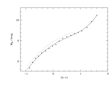
With the above conversions, the main sequence ($M_{R}$ vs $(b-r)$) can be approximated by a fourth order polynomial in the range $-1\leq(b-r)\leq 1.8$:

$$M_{R} = c_{0}+c_{1}\leavevmode\nobreak\ (b-r)+c_{2}\leavevmode\nobreak\ (b-r)^{2}$$ (4)

$$+ c_{3}\leavevmode\nobreak\ (b-r)^{3}+c_{4}\leavevmode\nobreak\ (b-r)^{4},$$

the parameters of which are:

$c_{0}=4.01236$       $c_{1}=4.12575$       $c_{2}=-1.89076$       $c_{3}=0.762053$       $c_{4}=0.341384$ ,

as shown in Fig. 1.

Figure 1: The mean main sequence from Lang (1992), converted to CADIS color $b-r$ and $R_{C}$ magnitude; the solid line is the fourth order polynomial (Eq. (4)). For the blue ($b-r<0.7$) metal-poor stars the mean main sequence is shifted towards fainter magnitudes.

One further complication arises due to the fact that the mean main sequence relation is valid strictly only for stars with solar metallicities, whereas our sample may contain stars spread over a wide range of different metalicities. For the blue stars ($b-r<0.7$), which are almost all halo stars (see Fig. 4), and therefore supposed to be metal-poor, we use the same main sequence relation, but shifted towards fainter magnitudes by $M_{R}=0.75^{mag}$ (see Fig. 1). This value is the mean deviation from the mean main sequence defined by the CNS 4 stars Jahreiß & Wielen  1997b of a subsample of 10 halo stars, for which absolute R magnitudes were available (Jahreiß, priv. com.).
The spread in a two color diagram $(b-r)$ versus $(r-i)$ (that is the CADIS color between $R_{C}$ and $I_{815}$ analog to Eq. (1)) becomes significant at $(b-r)\approx 1.0$, see Fig. 2. The maximal photometric error for the very faint stars is $0.15^{mag}$. Here metallicity effects will distort the relation between the measured $(b-r)$ colors and the spectral type (temperature) and thus lead to wrong absolute magnitudes, so we have to correct for metallicity in order to avoid errors in the photometric parallaxes.

Figure 2: The $b-r$ colors are projected along the ”isophotes” onto the mean main sequence track (solid line). For some of the very red stars ($b-r>1.8$), which are subject to the largest corrections, photometric errors are plotted.

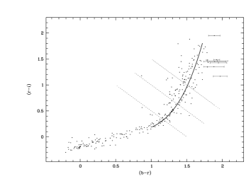
The $R_{C}$ filter is strongly affected by metallicity effects like absorption bands of TiO₂ and VO molecules in the stars’ atmosphere, whereas the $B_{C}$ and the medium-band filter $I_{815}$ (the wavelength of which was chosen in order to avoid absorption bands in cool stars) are not. So in a first approximation we can assume the ”isophotes” of varying metallicity in a $(b-r)$ versus $(r-i)$ two color diagram to be straight lines with a slope of $-1$, along of which we project the measured colors with $(b-r)\geq 1.0$ onto the mean main sequence track which in the interval $1.0\leq(b-r)\leq 1.8$ is defined by

$$(r-i) = 0.39\leavevmode\nobreak\ (b-r)_{{\rm corr}}^{4}-0.36\leavevmode\nobreak\ (b-r)_{{\rm corr}}^{3}$$ (5)

$$+ 0.09\leavevmode\nobreak\ (b-r)+0.06\leavevmode\nobreak\ .$$

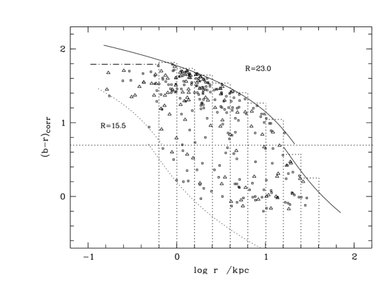
This projection implies that stars with $(b-r)_{{\rm corr}}\ga 1.8$ cannot exist in Fig. 3, which shows the spatial distribution of metallicity corrected $(b-r)_{{\rm corr}}$ colors (the limit is indicated by the dashed–dotted line).

Figure 3: Spatial distribution of metallicity corrected $(b-r)_{{\rm corr}}$. The solid line represents the distance dependent upper color limit at $R=23^{mag}$, the dotted line is the lower limit due to the selection criterium of the fields (no star brighter than $R\approx 15.5$). Since the metal-poor halo stars are intrinsically fainter, the color limits are shifted accordingly. The horizontal line denotes the cut between halo and disk stars, the dashed–dotted line indicates the cutoff at $(b-r)_{{\rm corr}}=1.8$ due to the metallicity correction. The different symbols refer to the different fields: squares – 16h field, triangles – 9h field.

Both the upper and lower magnitude limits lead to selection effects which have to be taken into account.
As one can see in Fig. 3 there is an bimodality of the observed color distribution. The accumulation of red stars in the upper left consists mainly of disk stars, and is separated by a void from the blue stars, which predominantly belong to the halo. Thus a crude disk-halo separation can be drawn by a color cut – we take stars with $(b-r)_{{\rm corr}}<0.7$ to be halo, stars with $(b-r)_{{\rm corr}}>0.7$ to be disk stars. In the following we will make use of this color cut to derive the distribution of the disk stars separately. In a second step, the distribution as a whole will be analysed. In Fig. 3 the cut is denoted by a dotted horizontal line.
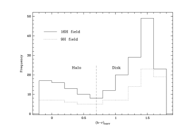
In the two fields we have analysed so far we find 95 halo and 178 disk stars, that is a factor of two more disk stars than predicted by the standard model Bahcall & Soneira (1980). This surplus of disk stars was already noted by Reid & Majewski (1993). Fig. 4 shows the distribution of the $(b-r)_{{\rm corr}}$ in the two fields under consideration.

Figure 4: Distribution of $(b-r)_{{\rm corr}}$ in the two fields, this bimodal distribution can be used to separate halo and disk stars by a color cut.

4 Density distribution of the stars

4.1 Completeness correction

As expected, the detection limit of absolute magnitudes (colors) is distance dependent (see Fig. 3).
We use the two-dimensional distribution of stars in the $(b-r)_{{\rm corr}}$ vs $\log r$ diagram (Fig. 3) to correct for this incompleteness in the following way: First, we divide the distance in logarithmic bins of 0.2 as indicated in Fig. 3 and count the stars up to the the upper color limit $(b-r)^{lim}$ (this is the distance dependent color (luminosity) limit, up to which stars can be detected. The metal-poor halo stars are intrinsically fainter (see paragraph 3)), thus the limits are shifted accordingly).
The nearest bins ($-0.8\leq\log r\leq-0.2$) are assumed to be complete. For the incomplete bins we multiply iteratively with a factor given by the ratio of complete to incomplete number counts in the previous bin, where the limit for the uncorrected counts is defined by the bin currently under examination ($j$):

$$N_{j}^{{\rm corr}}=N_{j}\prod_{i=1}^{j-1}(1+\frac{N_{i}^{{}^{\prime\prime}}}{N_{i}^{{}^{\prime}}})\leavevmode\nobreak\ ,$$ (6)

where $N_{j}$ is the number of stars in bin $j$, $N^{{}^{\prime}}$ is the number of stars in the previous bin ($j-1$), up to the limit given by the bin $j$, and $N^{{}^{\prime\prime}}$ is the number of stars from that limit up to the limit given by bin $j-1$, see also appendix.
With the poissonian errors $\sigma_{N}=\sqrt{N}$, $\sigma_{N^{{}^{\prime}}}=\sqrt{N^{{}^{\prime}}}$, and $\sigma_{N^{{}^{\prime\prime}}}=\sqrt{N^{{}^{\prime\prime}}}$ the error of the corrected number counts becomes:

$$\sigma^{2}_{N_{j}^{{\rm corr}}} = \sigma^{2}_{N_{j}}\prod_{i=1}^{j-1}\left(1+\frac{N_{i}^{{}^{\prime\prime}}}{N_{i}^{{}^{\prime}}}\right)^{2}$$ (7)

$$+ \sum_{i=1}^{j-1}\left[\left(\frac{1}{N_{i}^{{}^{\prime}}}\right)^{2}\sigma^{2}_{N_{i}^{{}^{\prime\prime}}}+\left(\frac{N_{i}^{{}^{\prime\prime}}}{N_{i}^{{}^{\prime}}}\right)^{2}\sigma^{2}_{N_{i}^{{}^{\prime}}}\right]$$

$$\cdot \prod_{m=1\atop m\not=j}^{j-1}\left(1+\frac{N_{i}^{{}^{\prime\prime}}}{N_{i}^{{}^{\prime}}}\right)$$

For a detailed deduction see appendix.
The completeness correction is done for each field separately.
With the corrected number counts the density in the logarithmic spaced volume bins ($V_{j}=\frac{1}{3}\omega(r_{j+1}^{3}-r_{j}^{3})$) can than be calculated according to

$$\rho_{j}=\frac{N^{{\rm corr}}_{j}}{V_{j}}=\frac{c\cdot N_{j}}{V_{j}}\leavevmode\nobreak\ ,$$ (8)

For every logarithmic distance bin we use the mean height $z$ above the Galactic plane $<z_{j}>=\sin b\cdot<r>$, where $<\log r>=\log r_{j}+(\log r_{j+1}-\log r_{i})/2=\log r_{i}+0.1\Rightarrow<r>=1.259r_{i}$.

4.2 Vertical density distribution

We first study the density distribution of the disk stars by taking only stars in the corresponding color interval into account. Although the color-cut at $(b-r)_{{\rm corr}}=0.7$ is a rather crude separation between disk and halo, we gain a clearer insight into the disk distribution since the contamination by halo stars is suppressed considerably.
As the nearest stars in our fields have still distances of about 200 pc the normalization at $z=0$ has to be established by other means: We take stars from the CNS4 Jahreiß & Wielen  1997b , which are located in a sphere with radius 20 pc around the sun.
The stars in our normalization sample are selected from the CNS4 by their absolute visual magnitudes, according to the distribution of absolute magnitudes of the CADIS disk stars ($6.5\leq M_{v}\leq 14.5$).
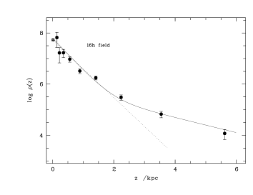
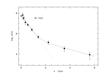
Fig. 5 shows the resulting density distribution of the disk stars in the two CADIS fields. The solid line represents a fit with a superposition of two exponentials, the dotted line is the fit for the thin disk component (the first seven data points). Obviously a single exponential is not a good description.
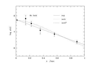
It was suggested to fit the thin disk with a secans hyperbolicus – the exponential is unphysical in that sense, that it is not continuously differentiable at $z=0$. A squared secans hyperbolicus (which represents a self-gravitating isothermal disk) can be proved not to fit the data very well – indicating that the stellar disk is in no way isothermal (the velocity dispersion depends on the spectral type).
The fits for the three functions under consideration:

$$\rho_{exp}(z) = n_{1}\exp(-z/h_{1})+n_{2}\exp(-z/h_{2})$$ (9)

$$\rho_{sech}(z) = n_{3}{\rm sech}(-z/z_{0})+n_{4}\exp(-z/h_{3})$$ (10)

$$\rho_{sech^{2}}(z) = n_{5}{\rm sech}^{2}(-z/\tilde{z_{0}})+n_{6}\exp(-z/h_{4})\leavevmode\nobreak\ .$$ (11)

are shown in Fig. 6, the corresponding parameters are given in Table 2.

Figure 5: Vertical density distribution of the disk stars ($b-r>0.7$) in the two fields, the normalisation (star) is given by data from the CNS4. The distribution shows clearly the contribution of the thick disk component – the solid line is a fit with a superposition of two exponentials, the dotted line is the single exponential fit for the thin disk component only.

As the secans hyperbolicus is a sum of two exponentials

$${\rm sech}(z/z_{0})=\frac{2}{\exp(z/z_{0})+\exp(-z/z_{0})}\leavevmode\nobreak\ ,$$ (12)

$z_{0}$ is not really a scaleheight, but has to be compared to $h_{1}$ by multiplying it with arcsech$\frac{1}{{\rm e}}\approx 1.65745$: $h_{1}^{\prime}=z_{0}\cdot 1.65745$ (cf. Tab. 2).

Figure 6: A secans hyperbolicus (dotted line) or a squared secans hyperbolicus (dashed line) can be shown to fit the thin disk equally well like an exponential (solid line). The normalisation is given by data from the CNS4.

Table 2: Fit parameter for the three fit functions

Parameter	16h field	9h field
$n_{1}$	5.06$\cdot 10^{7}$	5.84 $\cdot 10^{7}$
$n_{2}$	4.14 $\cdot 10^{6}$	6.23 $\cdot 10^{5}$
$h_{1}$	(280 $\pm$ 14)pc	(267 $\pm$ 9)pc
$h_{2}$	(1267 $\pm$ 74)pc	(1296 $\pm$ 116)pc
$n_{3}$	4.54 $\cdot 10^{7}$	5.19 $\cdot 10^{7}$
$n_{4}$	9.86 $\cdot 10^{6}$	1.02 $\cdot 10^{6}$
$z_{0}$	(172 $\pm$ 12)pc	(216 $\pm$ 8)pc
$h_{1}^{\prime}$	(286 $\pm$ 20)pc	(358 $\pm$ 13)pc
$h_{3}$	(1478 $\pm$ 30)pc	(1132 $\pm$ 84)pc
$n_{5}$	4.62 $\cdot 10^{7}$	5.4 $\cdot 10^{7}$
$n_{6}$	2.78 $\cdot 10^{6}$	1.37 $\cdot 10^{6}$
$\tilde{z_{0}}$	(352 $\pm$ 26)pc	(360 $\pm$ 13)pc
$h_{4}$	(1158 $\pm$ 112)pc	(1047 $\pm$ 71)pc

The errors of the scaleheights and corresponding parameters $z_{0}$ and $\tilde{z_{0}}$ are estimated by changing their values until $\chi^{2}$ increases by 1. We find that at $z=0$ the contribution of the thick disk component to the entire disk is $2\pm 4\%$.
Our values for the scaleheights lie within the range given by different authors in the literature. The proposed values for the exponential scaleheights of the thin disk range between 200 pc Kent et al.  1991 and 325 pc Bahcall & Soneira (1980). The parameters $\tilde{z_{0}}$ and $h_{4}$ we found in the 16 h field are equal within the errors to the values found by Gould et al (1997).

4.3 Density distribution in the halo

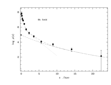
Fig. 7 shows the density distribution of all stars in the two CADIS fields. The dotted line is the secans hyperbolicus + exponential fit for the thin and thick disk components, the dashed line is a deVaucouleurs law. Although the space density corresponding to the $r^{1/4}$ law in projection has no simple analytic form Young (1976) it is possible to form expansions about the origin and the point at infinity. The latter expansion is valid for a large range of distances. An analytic approximation is Bahcall (1986):

$$\rho_{H}(z,b,l)=\rho_{0}\frac{\exp\left[-10.093\left(\frac{R}{R_{\odot}}\right)^{1/4}+10.093\right]}{\left(\frac{R}{R_{\odot}}\right)^{7/8}}$$

$$\cdot 1.25\frac{\exp\left[-10.093\left(\frac{R}{r_{\odot}}\right)^{1/4}+10.093\right]}{\left(\frac{R}{R_{\odot}}\right)^{6/8}},R<0.03R_{\odot}$$

$$\cdot \left[1-0.08669/(R/R_{\odot})^{1/4}\right],R\geq 0.03R_{\odot}$$

where $R=(R_{\odot}^{2}+z^{2}+\frac{z^{2}}{\tan^{2}b}-2R_{\odot}\frac{z}{\tan b}\cos l)^{1/2}$, $b$ and $l$ are Galactic latidude and longitude, the distance of the sun from the Galactic center $R_{\odot}=8$ kpc, $R=(x^{2}+z^{2})^{1/2}$, $x=(R_{\odot}^{2}+d^{2}\cos^{2}b-2R_{\odot}d\cos b\cos l)^{1/2}$, $z=d\sin b$. The dot-dashed is the sum of both halo and disk distribution function.
The density of halo stars extrapolated to $z=0$ is compared with the data from the CNS4 with an estimated error of $\approx 10$%. The stars are discriminated against disk stars by their metallicities and kinematics Fuchs & Jahreiß (1998). They are further selected according to the color cut of the CADIS halo stars ($(b-r\leq 0.7$).
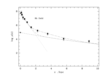
Fig. 8 shows the distribution of all stars in the range $z=0$ to $z=10$ kpc, the fit for a single exponential disk, the deVaucouleurs law, the sum of both, and the sum of the thin plus thick disk fit and the deVaucouleurs law. It is obvious that between $\approx 1.5$ kpc to 5.0  kpc the thick disk provides the predominant contribution to the overall distribution. Thus, the sum of thin disk and deVaucouleurs halo does not fit the distribution.

Figure 7: Density distribution perpendicular to the Galactic Plane, stars are data taken from the CNS4; the dotted line is the secans hyperbolicus plus exponential fit for the disk, the dashed line is a deVaucouleurs law and the dot-dashed the sum of both.

Figure 8: Distribution of all stars in the range $0\leq<z\leq 10$ kpc, the fit for a single exponential disk (dotted line) the deVaucouleurs law (short-dashed), the sum of both (dot-dashed), and the sum of the thin plus thick disk fit and the deVaucouleurs law (long-dashed).

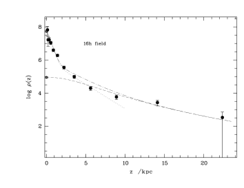
If we assume the sun to be 8 kpc away from the Galactic center and the normalisation $\rho_{0}$ to be fixed by the data from the CNS4, all parameters are completely determined. As can be seen in Fig. 7, the corresponding plots fit the distribution of the halo stars up to a distance of about 22 kpc above the Galactic plane.
The de Vaucouleurs law is an empirical description of the density distributions of stars in ellipticals, bulges of spirals and galactic halos de Vaucouleurs & Pence (1978) but it is equally justified to fit other distribution functions to the data: a smoothed power law fits the halo stars equally well Fuchs & Jahreiß (1998); Gould et al. (1998), see e.g. Fig. 9.

Figure 9: An inverse power law (broken line) can also be fitted to the data - in comparison with the a de Vaucouleurs law (solid line), shown here for the CADIS 9h field.

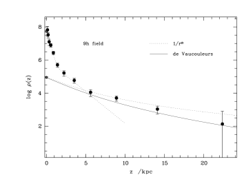
When applying the power-law fit, we add a further free parameter which describes the flattening of the halo:

$$\rho_{H}(z,b,l)=$$

$$\rho_{\odot}\!\left(\frac{r_{c}^{2}+r_{\odot}^{2}}{r_{c}^{2}+r_{\odot}^{2}+\frac{z^{2}}{tan^{2}b}-2r_{\odot}\frac{z}{\tan b}\cos l+\frac{z^{2}}{(c/a)^{2}}}\right)^{\alpha/2}\!,$$ (14)

with an arbitrarily chosen core radius of $r_{c}=1$ kpc.
We find an axial ratio $c/a$ of $(0.63\pm 0.07)$, with an exponent $\alpha=(2.99\pm 0.13)$.

5 The stellar luminosity function

The knowledge of the distribution function enables us to calculate the SLF for the thin disk stars. We selected the stars with distances less than 1.5 kpc. Beyond this point the contribution by thick disk and halo stars becomes dominant.
Although CADIS does not include a filter which is close to the Johnson-V, we calculate absolute visual magnitudes from the $R$ magnitudes to make comparison with literature easier. In the relevant magnitude intervall ($5\leq M_{V}\leq 14$, i.e $-1<(b-r)<1.8$) there holds a linear relation (see Sect. 3.1):

$$M_{V_{J}}=1.058\cdot M_{R_{C}}\leavevmode\nobreak\ .$$ (15)

We calculate an effective volume for every luminosity bin by integrating the distribution function along the line of sight, $r$, where the integration limits are given by the minimum between 1.5 kpc and the distance modulus derived for upper and lower limiting apparent magnitude:

$$V_{{\rm max}}^{{\rm eff}}=\omega\int\limits_{R_{{\rm min}}}^{R_{{\rm max}}}\nu(r,b)\leavevmode\nobreak\ r^{2}\leavevmode\nobreak\ dr\leavevmode\nobreak\ ,$$ (16)

where

$$R_{{\rm min}} = 10^{0.2(16^{{\rm mag}}-M_{R})-2.0}\leavevmode\nobreak\ ,$$

$$R_{{\rm max}} = {\rm min}(1.5\leavevmode\nobreak\ {\rm kpc},10^{0.2(23^{{\rm mag}}-M_{\rm R})-2.0})\leavevmode\nobreak\ .$$

The distribution function

$$\nu(r,b)=\exp(-r\sin b/h_{1})$$ (17)

is normalised to unity at $z=0$.
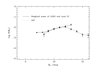
The weighted mean of the SLFs of the two CADIS fields is shown in Fig. 10, in comparison with the SLF of the stars inside a distance of 20 pc Jahreiß & Wielen  1997a , which is based on HIPPARCOS parallaxes.

Figure 10: The mean SLF of the two CADIS fields (solid line) and the local SLF Jahreiß & Wielen  1997a .

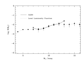
As can be seen from Fig. 10, the CADIS SLF is equal within the errors to the local SLF. Since the errors are dominated by Poissonian statistics, the error bars are small at the faint end, and larger at the bright end, complementary to the local SLF.
Thus the weighted mean of CADIS and local SLF which combines the large number of bright stars in the local sample with our superior sampling of faint stars (shown in Fig. 11) can be regarded as the most accurate determination of the SLF. The combined CADIS/local SLF keeps rising with constant slope to its limit at $M_{V}=13$. This is in pronounced contrast to previous determinations of the SLF based on faint star counts Stobie et al. (1989); Kroupa (1995). The discrepancy is demonstrated in Fig. 11 where we compare the combined SLF with the most recent photometric SLF based on HST observations Gould et al. (1998).
At this faint end both incompleteness and uncertainties of the exact location of the main sequence may introduce systematic errors which are hard to quantify.

Figure 11: The weighted mean of CADIS and local SLF in comparison with a photometric SLF which is based on HST observations Gould et al. (1998).

5.1 Implications for the mass function

The stellar mass function (SMF) can in principle be inferred from the SLF by converting the $M_{V}$ magnitudes of the disk stars ($r\leq 1.5$ kpc) into masses; this requires a mass-luminosity relation, for which we adopted the analytical fit taken from Henry et al. (1993, 1999). Their relation is valid for stellar masses from $0.08\,M/M_{\odot}$ to $2.0\,M/M_{\odot}$. If we count the stars in equally spaced mass intervals of $0.1$ and divide the number counts in the $j_{th}$ interval by the maximum effective volume (see Eq. (16)), calculated for the corresponding luminosity,
the SMF can be represented by a power law:

$$\Psi(M/M_{\odot})\propto\left[\frac{M}{M_{\odot}}\right]^{a}\leavevmode\nobreak\ .$$ (18)

From the data of the disk stars in the two CADIS fields we derived $a=-1.28\pm^{0.68}_{0.42}$ for [$0.2<M/M_{\odot}<1.1$]. Its slope is equal (within the errors) to the value proposed by Henry et al. (1993) ($a=-1$).

6 Summary and future prospects

Although the Calar Alto Deep Imaging Survey is designed as an extragalactic survey, we obtain a substantial set of multicolor-data about faint stars in the Galaxy. With the current filter set and exposure times the classification is reliable down to $M_{R}=23$.
From the $\approx 300$ stars we identified in two CADIS fields covering a total area of 1/15  ^∘, we deduced the density distribution of the stars up to a distance of about 20 kpc above the Galactic plane. The density distribution shows unambiguously the contribution of a thick disk component of the Galaxy with a scaleheight of $\approx 1.3$ kpc.
There has been discussion whether this ”thick disk” is introduced artificially by the assumption that all stars are on the main sequence Bahcall & Soneira (1984). Our present sample of very faint field stars does rule out this ambiguity: if there were any giant stars included in our data, they would have distances of about 250 kpc, thus their contribution to our sample can be neglected.
The density distribution in the halo, which essentially is corroborated by comparing the local density of CNS4 stars with the density between 5.5  kpc and 15  kpc above the Galactic plane from CADIS, is perfectly fit by a de Vaucouleurs’ law.
Based on our present, limited data set of 72 stars beyond z=5.5  kpc, it is equally well justified to fit an inverse power law with exponent $\alpha=2.99\pm 0.07$ to the data, with the axial ratio of the halo as an additional free parameter. The best fit value for the axial ratio is ($c/a=0.63\pm 0.07$).
Based on this knowledge of the density distribution, we determined the stellar luminosity function (SLF) for the disk stars. To this end, we confine our sample to stars with distances less than 1.5 kpc, for at this point the contribution of the thick disk and the halo population becomes predominant. Our result is within the errors indistinguishable from the local SLF Jahreiß & Wielen  1997a . Thus we conclude that the weighted average between the local SLF (containing predominantly stars at bright magnitudes ($M_{V}<10$)) and the CADIS SLF (with superior statistics at the faint end ($M_{V}>10$)) can be regarded as the best estimate of the SLF of the disk stars. The SLF continues to rise at least up to $M_{V}=13$, in contrast to most other photometric SLFs, which show a down-turn at $M_{V}=12$.
We regard this as a hint that incompleteness corrections and the closely connected issue of the ”true” sampling volume of these faint star counts might need some critical revision.
The stellar mass function (SMF) of the disk stars was derived by converting the visual magnitudes into masses Henry et al. (1993, 1999). For a power-law SMF $\Psi\propto(M/M_{\odot})^{a}$ we find a slope $a=-1.28\pm^{0.68}_{0.42}$. This is (within the errors) consistent with the slope proposed by Henry et al. (1993) ($a=-1$).
The main purpose of the present paper was to explore to what extent the faint star counts in CADIS can be used for determining the stellar density distribution and the stellar luminosity function of the disk. However, one should keep in mind that our present analysis is based only on about a quarter of of the entire Calar Alto Deep Imaging Survey data. In the entire sample which will contain eight fields of 1/30  ^∘each, we expect to identify a total of $\ga 1200$ stars with $R\leq 23$, of which 800 are supposed to be disk stars and 400 to be halo stars.
In addition with the complete multicolor data of the survey it should be possible to push the limit for a reliable star classification to $R=23.5$ or beyond.
As soon as better template spectra of stars with sub-solar metallicities become available, the currently rough correction for metallicity effect can be replaced by a more accurate metallicity dependent main sequence.
With this much more accurate determination of photometric distances and an at least 4-fold increased statistics it should be possible to adress the following issues concerning the density and luminosity function of the stars in the Galaxy:

• the scalelength $h_{r}$ of the density distribution of stars in the disk. This can be done if one takes the longitude dependent radial decrease of the density into account, e.g. the scaleheight measured in the CADIS 16h field ($l\approx 90\degr$) should be only very slightly affected by the radial density gradient, whereas the 9h field is suffering from a maximal radial decrease in density, so one measures an effective scaleheight $h_{{\rm eff}}$. Likely the star counts in the 18 h and 23 h field (at Galactic coordinates $b=30\degr$, $l=95\degr$, and $b=-43\degr$, $l=90\degr$, respectively, are only very slightly affected by the radial density gradient, so it should be possible to measure the ”true” scaleheights $h_{1}$ and $h_{2}$ for thin and thick disk component with high precision. From this, the counts in the 9h field and the 10 h field ($b=53\degr$, $l=150\degr$), we will deduce the scalelength $r_{i}=[1/h_{{\rm eff}}-1/h]^{-1}$.

• the axial ratio of a flattened halo and the exponent of the inverse power law with higher precision.

• a bulge – halo separation. By analysing the star counts in all eight fields it will be possible to separate the contribution of the bulge from the halo distribution.

• the slope of the SLF with higher precision. From the entire data set with limiting magnitude $R\geq 23.5$ we will be able to deduce the SLF down to $M_{V}\geq 14$ with good statistics and thus decide whether the features like the Wielen dip Wielen et al. (1983) at $M_{V}\approx 7$ and the apparent rise of the SLF beyond $M_{V}=12$ are real.
  

Appendix A Completeness correction

Since the first distance bin is assumed to be complete, we can iteratively correct the number counts in the next bins.
$N_{j}$ is the number of stars in bin $j$, $N^{{}^{\prime}}$ is the number of stars in the previous bin ($j-1$), up to the limit given by the bin $j$, and $N^{{}^{\prime\prime}}$ is the number of stars from that limit up to the limit given by bin $j-1$, as indicated in Fig. 12.
The division into $N^{{}^{\prime}}$ and $N^{{}^{\prime\prime}}$ is done to avoid correlated errors.

Figure 12: Schematic sketch of Fig. 3.

The first bin ($j=1$) is assumed to be complete ($N_{1}$). The corrected number $N_{2}^{{\rm corr}}$ in the second bin is then

$$N_{2}^{{\rm corr}}=N_{2}\cdot\left(\frac{N_{1}}{N_{1}^{{}^{\prime}}}\right)=N_{2}\left(\frac{N_{1}^{{}^{\prime}}+N_{1}^{{}^{\prime\prime}}}{N_{1}^{{}^{\prime}}}\right)=N_{2}\left(1+\frac{N_{1}^{{}^{\prime\prime}}}{N_{1}^{{}^{\prime}}}\right)\leavevmode\nobreak\ ,$$

and for the third bin

$$N_{3}^{{\rm corr}} = N_{3}\left(\frac{N_{2}^{{\rm corr}}}{N_{2}^{{}^{\prime}}}\right)=N_{3}\left(\frac{N_{1}}{N_{1}^{{}^{\prime}}}\right)\left(\frac{N_{2}}{N_{2}^{{}^{\prime}}}\right)$$

$$= N_{3}\left(\frac{N_{1}^{{}^{\prime}}+N_{1}^{{}^{\prime\prime}}}{N_{1}^{{}^{\prime}}}\right)\left(\frac{N_{2}^{{}^{\prime}}+N_{2}^{{}^{\prime\prime}}}{N_{2}^{{}^{\prime}}}\right)$$

$$= N_{3}\left(1+\frac{N_{1}^{{}^{\prime\prime}}}{N_{1}^{{}^{\prime}}}\right)\left(1+\frac{N_{2}^{{}^{\prime\prime}}}{N_{2}^{{}^{\prime}}}\right)\leavevmode\nobreak\ .$$

Thus this can generally be written as

$$N_{j}^{{\rm corr}}=N_{j}\prod_{i=1}^{j-1}\left(1+\frac{N_{i}^{{}^{\prime\prime}}}{N_{i}^{{}^{\prime}}}\right)$$ (19)

The errors of the number counts $N_{j}$, $N_{j-1}^{{}^{\prime}}$ and $N_{j-1}^{{}^{\prime\prime}}$ are independent of each other and thus Poissonian: $\sigma_{N_{j}}=\sqrt{N_{j}}$, $\sigma_{N_{j-1}^{{}^{\prime}}}=\sqrt{N_{j-1}^{{}^{\prime}}}$, $\sigma_{N_{j-1}^{{}^{\prime\prime}}}=\sqrt{N_{j-1}^{{}^{\prime\prime}}}$. Following Gaussian error propagation the error for the corrected number of stars in the second bin is

$$\sigma^{2}_{N_{2}^{{\rm corr}}} = \sigma^{2}_{N_{2}}+\left(\frac{N_{1}^{{}^{\prime\prime}}}{N_{1}^{{}^{\prime}}}\right)^{2}\sigma^{2}_{N_{2}}$$

$$+ \left(\frac{N_{2}}{N_{1}^{{}^{\prime}}}\right)^{2}\sigma^{2}_{N_{1}^{{}^{\prime\prime\prime\prime}}}+\left(\frac{N_{2}N_{1}^{{}^{\prime\prime}}}{N_{1}^{{}^{\prime\prime}2}}\right)^{2}\sigma^{2}_{N_{1}^{{}^{\prime}}}\leavevmode\nobreak\ ,$$

and for the third bin

$$\sigma^{2}_{N_{3}^{{\rm corr}}} = \sigma^{2}_{N_{3}}\left(1+\frac{N_{2}^{{}^{\prime\prime}}}{N_{2}^{{}^{\prime}}}\right)^{2}\left(1+\frac{N_{1}^{{}^{\prime\prime}}}{N_{2}^{{}^{\prime}}}\right)^{2}+$$

$$+ N_{3}^{2}\left(1+\frac{N_{1}^{{}^{\prime\prime}}}{N_{1}^{{}^{\prime}}}\right)\left[\left(\frac{1}{N_{2}^{{}^{\prime}}}\right)^{2}\sigma_{N_{2}^{{}^{\prime\prime}}}+\left(\frac{N_{2}^{{}^{\prime\prime}}}{N_{2}^{{}^{\prime}}}\right)^{2}\sigma^{2}_{N_{2}^{{}^{\prime\prime}}}\right]$$

$$+ N_{3}^{2}\left(1+\frac{N_{2}^{{}^{\prime\prime}}}{N_{2}^{{}^{\prime}}}\right)\left[\left(\frac{1}{N_{1}^{{}^{\prime}}}\right)^{2}\sigma_{N_{1}^{{}^{\prime\prime}}}+\left(\frac{N_{1}^{{}^{\prime\prime}}}{N_{1}^{{}^{\prime}}}\right)^{2}\sigma^{2}_{N_{1}^{{}^{\prime\prime}}}\right]$$

Thus the error of the completeness corrected counts in the $j^{th}$ bin is

$$\sigma^{2}_{N_{j}^{{\rm corr}}} = \sigma^{2}_{N_{j}}\prod_{i=1}^{j-1}\left(1+\frac{N_{i}^{{}^{\prime\prime}}}{N_{i}^{{}^{\prime}}}\right)^{2}$$ (20)

$$+ \sum_{i=1}^{j-1}\left[\left(\frac{1}{N_{i}^{{}^{\prime}}}\right)^{2}\sigma^{2}_{N_{i}^{{}^{\prime\prime}}}+\left(\frac{N_{i}^{{}^{\prime\prime}}}{N_{i}^{{}^{\prime}}}\right)^{2}\sigma^{2}_{N_{i}^{{}^{\prime}}}\right]$$

$$\cdot \prod_{m=1\atop m\not=j}^{j-1}\left(1+\frac{N_{i}^{{}^{\prime\prime}}}{N_{i}^{{}^{\prime}}}\right)\leavevmode\nobreak\ .$$

References

- Bahcall (1986) Bahcall, J. N., 1986, ARA&A, 24, 577
- Bahcall & Soneira (1980) Bahcall J. N., Soneira R. M., 1980, ApJS 44, 73
- Bahcall & Soneira (1984) Bahcall J. N., Soneira R. M., 1984, ApJS 55, 67
- Bertin & Arnouts (1996) Bertin E., Arnouts S., 1996, A&AS 117, 393
- de Vaucouleurs & Pence (1978) de Vaucouleurs G., Pence W. D., 1978, AJ 83, 1163
- Freeman (1992) Freeman K.C., 1992, in The Stellar Populations of Galaxies, Barbuy B., Renzini A. (eds.), Kluwer Academic Publishers, Dordrecht, IAU Symp.149, 65
- Fuchs & Jahreiß (1998) Fuchs B., Jahreiß H., 1998, A&A 329, 81
- Fuhrmann (1998) Fuhrmann K., 1998, A&A 338, 161
- Gilmore & Reid (1983) Gilmore G., Reid N., 1983, MNRAS 202, 1025
- Gould et al. (1997) Gould A., Bahcall J. N., Flynn C., 1997, ApJ 482, 913
- Gould et al. (1998) Gould A., Flynn C., Bahcall J. N., 1998, ApJ 503, 798
- Gunn & Stryker (1983) Gunn J. E., Stryker L. L., 1983, ApJS 52, 121
- Henry et al. (1993) Henry T. J., McCarthy D. W. Jr., 1993, AJ 106, 773
- Henry et al. (1999) Henry T. J., Franz O. G., Wasserman L. H. et al., 1999, ApJ 512, 864
- (15) Jahreiß H., Wielen R., 1997a, in HIPPARCOS ’97. Presentation of the HIPPARCOS and TYCHO catalogues and first astrophysical results of the Hipparcos space astrometry mission., Battrick B., Perryman, M.A.C., Bernacca P.L., (eds.), ESA SP-402, Noordwÿk p. 675
- (16) Jahreiß H., Wielen R., 1997b, in HIPPARCOS ’97. Presentation of the HIPPARCOS and TYCHO catalogues and first astrophysical results of the Hipparcos space astrometry mission., Battrick B., Perryman, M.A.C., Bernacca P.L., (eds.) , ESA SP-402, Noordwÿk , p. 587
- (17) Kent, S. M., Dame, T. M., Fazio, G., 1991, ApJ, 378, 131
- Kroupa (1995) Kroupa P., 1995, ApJ 453, 350
- Lang (1992) Lang K.R., 1992, Astrophysical Data I, Planets and Stars, Berlin, Springer-Verlag
- Meisenheimer & Röser (1986) Meisenheimer K., Röser H.-J., 1986, in The Optimization of the Use of CCD Detectors in Astronomy, Baluteau J.-P., D’Odorico S., (eds.), (ESO-OHP:Garching bei München), p.227
- Meisenheimer et al. (1998) Meisenheimer K., Beckwith S., Fockenbrock R., et al., 1998, in The Young Universe: Galaxy Formation and Evolution at Intermediate and high Redshift, D’Odorico, S., Fontana, A., Giallongo E., (eds.), ASP Conf. Ser., Vol. 146, p. 134
- Norris (1998) Norris, J.E., 1998 in Galaxy Evolution: Connecting the Distant Universe with the local Fossil Record, Spite M. (eds.), Kluwer Academic Publishers, Dordrecht, in press
- Oke (1990) Oke, J. B., 1990, AJ, 99, 1621
- Reid & Majewski (1993) Reid I.N., Majewski S.R., 1993 ApJ 409, 635
- Reid et al. (1996) Reid I.N., Yan L., Majewski S., et al., 1996, AJ 112, 1472
- Reid et al. (1997) Reid I.N., Gizis J.E., Cohen J.G., et al., 1997 PASP 109, 559
- Stobie et al. (1989) Stobie R. S., Peacock J. A., Ishida K., 1989, MNRAS 276, 709
- Walsh (1995) Walsh, J. 1995, Optical and uv spectrophotometric standard stars. http://www.eso.org/observing/standards/spectra.
- Wielen et al. (1983) Wielen, R., Jahreiß, H., Kruger, R., 1983, in The Nearby Stars and the Stellar Luminosity Function, Davis Philip A.G., Upgren (eds.), Davis Press, Schenectady, N.Y., IAUC 76, p.163
- Wolf (1998) Wolf, C., 1998, Ph.D. thesis, Ruprecht-Karls-Universität Heidelberg
- Wolf et al. (1999) Wolf, C., Meisenheimer, K., Röser, H.-J., et al., 1999, A&A 343, 399
- Young (1976) Young P.A., 1976, AJ 81, 807