Implementing Feedback in Simulations of Galaxy Formation:
A Survey of Methods

Abstract

We present a detailed investigation of a number of different approaches to modelling feedback in simulations of galaxy formation. Gas-dynamic forces are evaluated using Smoothed Particle Hydrodynamics (SPH). Star formation and supernova feedback are included using a three parameter model which determines the star formation rate (SFR) normalization, feedback energy and lifetime of feedback regions. The star formation rate is calculated for all gas particles which fall within prescribed temperature, density and convergent flow criteria, and for cosmological simulations we also include a self-gravity criterion for gas particles to prevent star formation at high redshifts. A Lagrangian Schmidt law is used to calculate the star formation rate from the SPH density. Conversion of gas to stars is performed when the star mass for a gas particle exceeds a certain limit, typically half that of the gas particle. Feedback is incorporated by returning a precalculated amount of energy to the ISM as thermal heating. We compare the effects of distributing this energy over the smoothing scale or depositing it on a single particle. Radiative losses are prevented from heated particles by adjusting the density used in radiative cooling so that the decay of energy occurs over a set half-life, or by turning off cooling completely and allowing feedback regions a brief period of adiabatic expansion. We test the models on the formation of galaxies from cosmological initial conditions and also on isolated disk galaxies. For isolated prototypes of the Milky Way and the dwarf galaxy NGC 6503 we find feedback has a significant effect, with some algorithms being capable of unbinding gas from the dark matter halo (‘blow-away’). As expected feedback has a stronger effect on the dwarf galaxy, producing significant disk evaporation and also larger feedback ‘bubbles’ for the same parameters. In the critical-density CDM cosmological simulations, evolved to a redshift $z=1$, we find the reverse to be true. Further, feedback only manages to produce a disk with a specific angular momentum value approximately twice that of the run with no feedback, the disk thus has an specific angular momentum value that is characteristic of observed elliptical galaxies. We argue that this is a result of the extreme central concentration of the dark halos in the standard CDM model and the pervasiveness of the core-halo angular momentum transport mechanism (even in light of feedback). A simulation with extremely violent feedback, relative to our fiducial models, leads to a disk that resembles the other simulations at $z=1$ and has a specific angular momentum value that is more typical of observed disk galaxies. At later times, $z=0.5$, a large amount of halo gas which does not suffer an angular momentum deficit is present, however the cooling time is too long to accrete on to the disk. We further point out that the disks formed in hierarchical simulations are partially a numerical artifact produced by the minimum mass scale of the simulation acting as a highly efficient ‘support’ mechanism. Disk formation is strongly affected by the treatment of dense regions in the SPH method. The problems inherent in the treatment of high density regions in SPH, in concert with the difficulty of representing the hierarchicial formation process, means that realistic simulations of galaxy formation require far higher particle resolution than currently used.

1. Introduction

A detailed understanding of galaxy formation in hierarchically clustering universes remains one of the primary goals of modern cosmology. Whereas on large scales the clustering of matter is determined almost solely by gravitational forces, a large number of physical processes contribute to galaxy formation. Further complication is evident in that a significant number of these processes cannot be modelled from first principles in a simulation of galaxy formation, the main example of this being star formation.

Analytic and semi-analytic theories of galaxy formation are well-developed (see White 1994, for an overview). The theoretical framework for studying the condensation of baryons in dark matter halos was laid out by White & Rees (1978) following the foundational work on hierarchical clustering by Peebles (1980, and references therein). White and Rees illuminated the fact that for baryons condensing in dark matter halos of sub-galactic ($\gtrsim 10^{6}$ $\rm\thinspace M_{\odot}$) size the cooling time of the gas is always shorter than the free-fall collapse time. In a related paper, Fall & Efstathiou (1980) demonstrated that disk galaxies could be formed in a hierarchical clustering model, provided that the gas maintains its angular momentum. Later work by White & Frenk (1991) further developed this hierarchical clustering model and identified the cooling catastrophe for CDM cosmologies. The cooling catastrophe is caused by the large mass fraction in small high-density halos at early times. The gas resident in these halos cools on the time-scale of a Myr, thus precipitating massive star formation very early on in the development of the CDM cosmology (at odds with the observations of our Universe). To circumvent this problem White & Frenk introduced star formation and the associated feedback from supernovae and showed that, given plausible assumptions, the cooling catastrophe can be avoided. The main deficiency in the semi-analytic programmes is that they cannot describe the geometry of mergers which is exceptionally important in the assembly of galaxies.

Smoothed Particle Hydrodynamic simulations of galaxy formation (Katz (1992); Navarro & White (1994); Evrard, Summers & Davis (1994), for example) detail the hierarchical merging history, but have been limited in terms of resolution. Achieving high resolution is particularly difficult. Since galaxy formation is affected by long range tidal forces, the simulation must be large enough to include these, which in turn enforces a low mass resolution. Two solutions to this problem exist; the first samples the long range fields using lower particle resolution than the main simulation region (the multiple mass technique, Porter 1985) while the second includes the long range fields as a pre-calculated low resolution external field (e.g. Sommer-Larsen, Gelato & Vedel (1998)). Simulations performed in this manner represent lengths scales from 50 Mpc to 1 kpc, a dynamic range of $5\times 10^{4}$.

It is well known that in SPH simulations it is comparatively easy to form flattened disk structures resembling disk galaxies. However, the resulting gaseous structures are deficient in angular momentum (see Navarro, Frenk & White 1995, for a comparison of a number of simulations to observed galaxies). The loss of angular momentum occurs during the merger process as dense gas cores lose angular momentum to the dark matter halos (see Barnes 1992, for an explanation of the mechanism). This is a very significant problem since a fundamental requirement of the disk formation model, presented in Fall & Efstathiou (1980), is that the gas must maintain a similar specific angular momentum to the dark matter to form a disk. The solution to this problem is widely believed to be the inclusion of star formation and feedback from supernovae and stellar winds. By including these effects the gas should be kept in a more diffuse state which consequently does not suffer from the core-halo angular momentum transport problem. Notably, a recent letter by Dominguez-Tenreiro, Tissera & Saiz (1998), based upon analytic work by Christodoulou, Shlosman & Tohline (1995) and van den Bosch (1998), has shown that the inclusion of star formation may go some way in helping to resolve the angular momentum problem. They suggest that a second mechanism, bar formation, also contributes to the loss of angular momentum within the disk. Including a photoionizing background (Efstathiou 1992) appears to make the problem slightly less severe (Sommer-Larsen, Gelato & Vedel 1998) but this is the subject of debate; for a conflicting viewpoint see Navarro & Steinmetz (1997).

Individual supernovae cannot be modelled in galaxy formation simulations. Consequently, there is no a priori theory for how feedback energy should be distributed in the simulation. A decision must be made whether feedback energy should be passed to the thermal or kinetic sector of the simulation. As a direct result of this ‘freedom’, a number of different algorithms for the distribution of feedback energy have been proposed (Katz (1992); Navarro & White (1993); Mihos & Hernquist (1994) for example). Since the interstellar medium is multi-phase (McKee & Ostriker (1977)), the feedback process should ideally be represented as an evaporation of molecular clouds. Note that in a single-phase model, the analogue of the cloud evaporation process is thermal heating. A seminal attempt at representing this process has been made by Yepes et al. (1997), and recently Hultman and Pharasyn (1999) have adapted the Yepes et al. model to SPH. At the moment it is unclear how well motivated these models are since (1) they must make a number of assumptions about the physics of the ISM and (2) they are not truly multiphase, since the dynamics are still treated using a single phase. Consequently, given the uncertainties inherent in multiphase modeling, the investigation presented here explores a single phase model.

As a first approximation, the star formation algorithms can be divided into three groups. The first group contains algorithms which rely upon experimental laws to derive the star formation rate (Mihos & Hernquist (1994), for example). The second group contains those which predict the SFR from physical criteria (Katz (1992), for example). The third group is comprised of algorithms which do not attempt to predict the SFR, but instead set a density criterion for the gas so that when this limit is reached the gas is converted into stars (Gerritsen & Icke (1997), for example). In this work the first approach is taken.

Given that feedback occurs on sub-resolution scales, it is difficult to decide upon the scale over which energy should be returned. However, SPH incorporates a minimum scale automaticallythe smoothing scale. Katz (1992) was the first to show that simply returning a specified amount of energy to the ISM is ineffective: the characteristic time-scale of radiative cooling at high density is far shorter than the simulation dynamical time-scale. This is, at least partially, another drawback of trying to model sub-resolution physics at the edge of the resolution scale. Further, the strong disparity between time-scales means that not only are length scales sub-resolution, so is the characteristic temporal evolution. This point has been made several times in relation to simulations with cooling (e.g. Katz 1992) but it seems even more important in the context of models with feedback. Thus, in an attempt to circumvent this problem, a new thermal feedback model is presented in which the radiative losses are reduced by changing the density used in the radiative cooling equation. The density used is predicted from the ideal gas equation of state and then integrated forward, decaying back to the SPH density (in a prescribed period). The effect of preventing radiative losses using a brief adiabatic period of evolution for the feedback region (Gerritsen (1997)) is also examined. An alternative method of returning thermal energy is to heat an individual SPH particle (Gerritsen (1997)). This method has been shown to be effective in simulations of isolated dwarf galaxies. The final mechanism considered is one that attempts to increase the energy input from SN to account for the high radiative losses. Mechanical feedback boosts are not considered for the following reasons; (1) parameters that are physically motivated (e.g. feedback efficiency of 10%) produce too much velocity dispersion, and (2) the method makes no account for force softening.

The response of the (simulated) ISM to a single feedback event is examined to gain an understanding of the qualitative and quantitative performance of each feedback algorithm. To determine whether the parameters of the star formation are more important than the dynamics of the simulation, an exploration of the parameter space of one of the algorithms is undertaken. Since feedback is expected to have a more significant effect on dwarf systems (due to the lower escape velocity) the effect of the feedback algorithms on a Milky Way prototype is contrasted against a model of the dwarf galaxy NGC 6503. Following this investigation, a series of cosmological simulations is conducted to examine whether the conclusions from the isolated simulations hold in a cosmological environment. Particular attention is paid to the rotation curves and angular momentum transport between the galaxy and halo.

The structure of the paper is as follows: In section 2, important features of the numerical technique are reviewed. In sections 3-4, the star formation prescription is presented and a detailed analysis of its performance on isolated test objects presented conducted. Results from simulations are reviewed in section 4, and a summary of the findings is given in section 6.

2. Numerical Method

An explicit account of the numerical method, including the equation of motion and artificial viscosity used, is presented in Thacker et al. (1998). The code is a significant development of the publically available HYDRA algorithm (Couchman, Thomas & Pearce 1995). The main features of the method are summarized for clarity. Gravitational forces are evaluated using the adaptive Particle-Particle, Particle-Mesh algorithm (AP³M, Couchman (1991)). Hydrodynamic evolution is calculated using SPH. Notable features of algorithm relevant to the hierarchical simulations follow,

• The neighbour smoothing is set to attempt to smooth over 52 neighbour particles, usually leading to a particle having between 30 and 80 neighbours. This number of neighbors assures a stable integration and reduces concern over the relative fluctuation in neighbor counts.

• The minimum hydrodynamic resolution scale is set by $h_{min}=\epsilon/2$ where $\epsilon$ is the gravitational softening. If the minimum gravitational resolution is $2\epsilon$ and the minimum hydrodynamic resolution $4h_{min}$ then the two of them match with this definition of $h_{min}$.

• Once the smoothing length of a particle reaches $h_{min}$, all particles within $2h_{min}$ are smoothed over. Thus at this scale the code changes from an adaptive to nonadaptive scheme. This avoids mismatched gravitational and hydrodynamic forces at scales close to that of the resolution (Bate & Burkert (1997)).

Radiative cooling is implemented using an assumed 5% $Z_{\odot}$ metallicity. The precise cooling table is interpolated from Sutherland and Dopita (1993). Radiative cooling is calculated in the same fashion as discussed in Thomas & Couchman (1992).

3. Star Formation Prescription

3.1. Implementation details

The star formation algorithm is based on that presented in Mihos and Hernquist (1994). Kennicutt (1998) has presented a strong argument that the Schmidt Law, with star formation index $\alpha=1.4\pm 0.15$, is an excellent model. It characterizes star formation over five decades of gas density, although it does exhibit significant scatter.

For computational efficiency, a Lagrangian version of the Schmidt Law is used, that corresponds to a star formation index $\alpha=1.5$,

$${dM_{*}\over dt}=C_{\it sfr}\;\rho_{g}^{1/2}\;M_{g},$$ (1)

where $C_{\it sfr}$ is the star formation rate normalization, the $g$ subscripts denotes gas and the $*$ subscript stars. Assuming approximately constant volume over a time-step, both sides may divided by the volume and the standard Schmidt Law with index $\alpha=1.5$ is recovered. A value of $\alpha=1.5$ is preferred since it leads to the square root of the gas density, which is numerically efficient and the value is within the error bounds. As written the constant $C_{\it sfr}$ has units of $\rho^{-1/2}t$, but can be made dimensionless by multiplying by $(4\pi G)^{1/2}$. Hence, equation 1 may be written with dimensionless constants, leading to the following form,

$${dM_{*}\over dt}=\sqrt{4\pi G}\,c^{*}\;\rho_{g}^{1/2}\;M_{g}=\frac{c^{*}M_{g}}{t_{ff}},$$ (2)

where $c^{*}$ is the dimensionless star formation rate (Katz (1992)). The range for this parameter is reviewed in section 3.4. Limiting the star formation rate by the local cooling time-scale was not considered. The reason for this is that typically the cold dense cores which form stars are at the effective temperature minimum of the simulation for non-void regions, namely $10^{4}$ K, which corresponds to the end of the radiative cooling curve.

Star formation is allowed to proceed in regions that satisfy the following criteria,

1. the gas exceeds the density limit of $2\times 10^{-26}\rm{g\;cm}^{-3}$

2. the flow is convergent, ($\nabla.{\bf v}<0$)

3. the gas temperature is less than $3\times 10^{4}$ K

4. the gas is partially self-gravitating, $\rho_{gas}>0.4\rho_{dm}$

The first criterion associates star formation with dense regions (regardless of the underlying dark matter structure). The second criterion is included to link star formation with regions that are collapsing. The third prevents star formation from occurring in regions where the average gas temperature is too high for star formation. The final criterion is particularly relevant to cosmological simulations since it limits star formation to regions where the dynamics are at least partially determined by the baryon density. Since the mass scales probed by the simulation are considerably larger than the mass scales of self-gravitating cores in which star formation would occur, we use a pre-factor of 0.4 to help compensate for this disparity.

Representing the growth of the stellar component of the simulation requires compromises. It is clearly impossible to add particles with masses $dM_{*}$ at each time-step since this would lead to many millions of small particles being added to the simulation. Alternatively, a gas particle may be viewed as having a fractional stellar mass component, i.e. the particle is a gas-star hybrid (in the terminology of Mihos & Hernquist (1994)). Thus, as gas is turned into stars, the stellar mass increases while the gas mass decreases. Mihos and Hernquist take this idea to its limit by only calculating gas forces using the gas mass of a particle (gravitational forces are unaffected because of mass conservation). A drawback of this method is that it still enforces a collisional trajectory on the collisionless stellar content of a particle. While this is a good description of real physics, since stars take a number of galactic rotations to depart from the gas cloud in which they are born, it is in strong disagreement with what would happen to collisional and collisionless particles in a simulation. To decide when to form stars, Katz (1992) and Steinmetz & Muller (1994, 1995) use a star formation efficiency. Once the star mass of the gas particle reaches a set (efficiency) percentage of the gas particle mass then a star particle is created with that mass value. This also leads to the potential spawning of very many gas particles. As a compromise, the scheme used in this work is as follows: Once $\dot{M}_{*}$ has been evaluated, the associated mass increase over the time-step is added to the ‘star mass’ of the hybrid gas-star particle. Note, in this model the ‘star mass’ is a ‘ghost’ variable and does not affect dynamics in any way, i.e. until the star particle is created the particle is treated as entirely gaseous when calculating hydrodynamic quantities. Two star particles (of equal mass) can be created for every gas particle. This ensures that feedback events occur frequently since we do not have to wait for the entire gas content of a region to be consumed before feedback occurs, and at the same time prevents the spawning of too many star particles. The creation of a star particle occurs when the star mass of a gas-star particle reaches one half that of the mass of the initial gas particles. The gas-star particle mass is then decremented accordingly. The second star particle is created when the star mass reaches 80% of half the initial gas mass. SPH forces are calculated using the total mass of the hybrid particles. Note, in all the following sections, “gas particle” should be interpreted meaning “gas-star hybrid particle”. These assumptions yield a star formation algorithm where each gas particle has a star formation history. This assumption is motivated because cloud complexes in any galaxy have an associated star formation history.

There are two notable drawbacks to this algorithm. Firstly, since star particles are only formed when the star mass exceeds a certain threshold there is a delay in forming in stars. As a consequence, prior to the star particle being formed, the SPH density used in the calculation of the SFR will be overestimated. By selecting the star mass to be one half that of the gas mass this problem is reduced, but it is not removed. Secondly, until the first star particle is spawned, the trajectory of the stellar component is entirely determined by the gas dynamics.

Once a star particle is created the associated feedback must be evaluated. A simple prescription is utilized, namely that for every $100M_{\odot}$ of stars formed there is one supernovae which contributes $10^{51}$ erg to the ISM. This value is used in Sommer-Larsen et al. (1998), and feeds back $5\times 10^{15}$ erg g^-1 of star particle to the surrounding ISM. Since this value is a specific energy, a temperature can be associated with feedback regions (see section 3.2). Navarro & White (1993), using a Salpeter IMF, with power law slope 1.5 and mass cut-offs at 0.1 and 40 $M_{\odot}$, derive that $2\times 10^{15}$ erg g^-1 of star particle created is fed back to the surrounding gas. The actual value is subject to the IMF, but scaling between values can be achieved using a single parameter which we label $e^{*}$. For $e^{*}=1$ the energy return is $5\times 10^{15}$ erg g^-1, while $e^{*}=0.4$ gives the Navarro & White value. Only brief attention is paid to changing this parameter since it is more constrained than the others in the model. Variations in metallicity caused by the feedback process (Martel & Shapiro (1998)) are not considered, as this involves a complicated feedback loop involving the gas density and cooling rate.

3.2. Energy feedback

The following sections describe each of the feedback algorithms considered.

3.2.1 Energy smoothing (ES)

The first of the methods is comparatively standard: the total feedback energy is returned to the local gas particles. For simplicity in the following argument, it is assumed a tophat kernel is used to feedback the energy over the nearest neighbour particles. The number of neighbours is constrained to be between 30 to 80 which may divorce the feedback scale from the minimum SPH smoothing scale set by $h_{min}$. This occurs in the densest regions where the average interparticle spacing becomes significantly less than $h_{min}$. This actually renders feedback more effective in these regions than it would be if all the energy were returned to the particles with in $2h_{min}$ region, but the effect is not significant. Given these assumptions for star formation, and working in units of internal energy, it is possible to evaluate the temperature increase, $\Delta T$ of a feedback region as follows,

$$\Delta T={2\over 3}{\mu m_{p}\over k}{E_{SN}M_{*}\over N_{s}M_{g}},$$ (3)

which given $N_{s}=52$, $E_{SN}=5\times 10^{15}\;\rm{erg}\;\rm{g}^{-1}$, and $M_{*}/M_{g}=1/2$ yields,

$$\Delta T\simeq 2.4\times 10^{7}{M_{*}\over N_{s}M_{g}}\simeq 2.3\times 10^{5}\;\rm{K}.$$ (4)

Clearly this boost may be increased or decreased by altering any one of the variables $E_{SN}$, $N_{s}$ and the ratio $M_{*}/M_{g}$. Keeping $E_{SN}$ constant, but reducing $N_{s}$ to 32 and increasing $M_{*}/M_{g}$ to 1 would yield $\Delta T\simeq 7\times 10^{5}\;\rm{K}$, demonstrating the sensitivity of feedback to the SPH smoothing scale.

3.2.2 Single particle feedback (SP)

Alternatively, all of the energy may be returned to a single SPH particle. Gerritsen (1997) has shown that this is an effective prescription in simulations of evolved galaxies, yielding accurate morphology and physical parameters. In this case the temperature boost is trivially seen to be

$$\Delta T\simeq 2.4\times 10^{7}\rm{K}.$$ (5)

as $N_{s}=1$ and $M_{*}/M_{g}=1$. There is one minor problem in that when the gas supply is exhausted, the mechanism has no way of returning the energy (unless one continues to make star particles of smaller and smaller masses). As a compromise the nearest SPH particle is found and the energy is given to this particle.

3.2.3 Temperature smoothing (TS)

The final feedback mechanism considered is one that accounts for the fast radiative losses by increasing the energy input. The first step is to calculate the temperature a single particle would have if all the energy were returned to it (as in the SP model). Then this value is smoothed over the local particles using the SPH kernel. This method leads to a vastly higher energy input than the others and represents a case of extreme feedback (essentially 52 times the ES feedback). For the isolated simulations, the cooling mechanism (see below) was not adjusted in this model since the feedback regions in the disk have cooling time of several time-steps (at least 10). In the cosmological simulations, the alternative cooling mechanisms were considered since the cooling time is only a few time-steps (Katz (1992); Sommer-Larsen, Gelato & Vedel (1998)).

3.2.4 Preventing immediate radiative energy losses

As was previously discussed, Katz (1992) was the first to show that feedback energy returned to the ISM is radiated away extremely quickly in high density regions. This is a result of the characterisitic dynamical time of the simulation being far longer than that of cooling.

The first method for preventing the immediate radiative loss of the feedback energy is to alter the density value used in the radiative cooling mechanism. This change is motivated by Gerritsen’s (1997) tests on turning off radiative cooling in regions undergoing feedback. Assuming pressure equilibrium between the ISM phases (which is not true after a SN shell explodes but is a good starting point) one may derive the estimated density that the region would have after the SN shell has exploded. If the local gas energy is increased by $E_{SN}$, then the perfect gas equation of state yields

$$\rho_{est}={E_{i}\rho_{i}\over E_{i}+E_{SN}}.$$ (6)

Following a feedback event the estimated density is allowed to decay back to it’s local SPH value with a half-life $t_{1/2}$.

Fig. 1.—Evolution of the cooling density and the SPH density following a single feedback event in the ESna scheme. $t_{1/2}=5$ Myr, and clearly the values converge within $2t_{1/2}$. Note the small initial drop in the SPH density in response to the feedback energy, followed by a slower expansion. The initial cooling density is approximately 5% of the SPH density, consistent with the feedback temperature of $2\times 10^{5}$ K in an ambient 10,000 K region.

To calculate the decay rate (i.e. to predict the cooling density at the time-step $n+1$ from that at time-step $n$) the following function is used

$$\footnotesize\rho_{cool}^{n+1}=\cases{\rho_{cool}^{n}+dt\times\Delta\rho^{n}(t_{f}^{2}/t_{1/2}^{3})e^{-0.33(t_{f}/t_{1/2})^{3}},&$t_{f}\leq t_{1/2}$;\cr\vspace{5pt}\cr\rho_{SPH}^{n}-\Delta\rho^{n}e^{-0.693dt/t_{1/2}},&$t_{1/2}\leq t_{f}<3t_{1/2}$;\cr\vspace{5pt}\cr\rho_{SPH}^{n+1},&$3t_{1/2}\leq t_{f}$ ,}$$ (7)

where $t_{f}$ is time since the feedback event occurred, $\Delta\rho^{n}=\rho_{SPH}^{n}-\rho_{cool}^{n}$, and $dt$ is the time-step increment. Once a region passes beyond $3t_{1/2}$, the cooling density is forced to be equivalent to the SPH density, although usually the values converge within $2t_{1/2}$. This comparatively complex function was chosen because in a simple exponential decay model, the cooling density increases by the largest amount immediately following the feedback event. To have any effect the cooling density must be allowed to persist at its low value for a reasonable period of time. In figure 1 the two densities calculated after a single feedback event are compared. This cooling mechanism is denoted by a suffix na (for non-adiabatic) on the energy input acronym. Springel and White (in prep) have considered a similar model (Pearce, private communication).

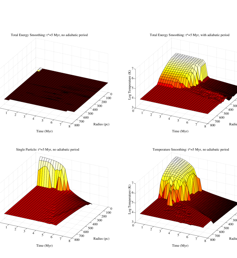
Figure 2.— Evolution of the cooling density and the SPH density following a single feedback event in the ESna scheme. $t_{1/2}=5$ Myr, and clearly the values converge within $2t_{1/2}$. Note the small initial drop in the SPH density in response to the feedback energy, followed by a slower expansion. The initial cooling density is approximately 5% of the SPH density, consistent with the feedback temperature of $2\times 10^{5}$ K in an ambient 10,000 K region.

Gerritsen allowed his SPH particles to remain adiabatic for $3\times 10^{7}$ years, approximately the lifetime of a $8M_{\odot}$ star. It is difficult to argue what this value should be and hence the $t_{1/2}$ parameter space was explored. Note that if during the decay period another feedback event occurs in the local region, the density value used is the minimum of the current decaying one and the new calculated value.

As a second method for preventing radiative losses Gerritsen’s idea was utilized: make the feedback region adiabatic. This is easily achieved in our code by using the same mechanism that calculates the estimated density value. Provided the estimated density value is less than half that of the local SPH value then the particle is treated as adiabatic. Above this value the estimated density is used in the radiative cooling equation. This cooling mechanism is denoted with a suffix a.

3.3. Comparison of methods

To test each of the feedback methods and gain insight into their effect on the local ISM, a single feedback event was set up within a prototype isolated Milky Way galaxy. The evolution of the particles within $3h$ of the feedback event were followed. The time evolution of the temperature versus radius for each scheme is shown in figure 2.

3.3.1 Qualitative discussion

The adjusted cooling mechanism has little effect on the ES run because the estimated density is not low enough to increase the cooling time significantly beyond the length of the time-step. Including a prefactor of 0.1 in the equation, so that the estimated density is significantly lower, does increase the cooling time sufficiently. However, since introducing the adiabatic phase allows the feedback energy to induce expansion, we prefer this method, rather than trying to adjust the estimated density method. For the SP run the density reduction is much higher (since the total energy, $E_{SN}$, is applied to the single particle) and hence the mechanism does allow the particle to remain hot. There is little perceptible difference between the SPa and SPna profiles.

Both SP feedback, TS, and ESa induce noticeable expansion of the feedback region. Thus after the heat input has been radiated away, the continued expansion introduces adiabatic cooling (since the temperature of the region falls below the $10,000$ K cut off of the cooling curve). It is particular noticeable in the TS plot where the low temperature plateau continues to widen quite drastically and this is manifest in the simulation with the appearance of a large bubble in the disk. Caution should be exercised in interpreting these bubbles in any physical manner, since their size is set solely by the resolution scale of the SPH. ESa also produces bubbles, but due to the lower temperature there is less expansion. Single particle feedback produces the smallest bubbles and often ejects the hot particle vertically from the disk. This occurs with regularity since the smoothing scale is typically larger than the disk thickness: if the hot particle resides close to the edge of the disk the pressure forces from the surrounding particles will be asymmetric resulting in a strong ‘push’ out of the disk. Note that this is phenomenologically similar to the mechanism by which SN gas is ejected from disks (McKee & Ostriker (1977)), although this should not be over-interpreted.

The only scheme which stands out in this investigation is ESna: the cooling mechanism fails to prevent drastic radiative losses. The remainder of the algorithms produce an effect on both the thermal properties of the ISM and its physical distribution.

3.3.2 Effect of methods on time-step criterion

Since our code does not have multiple time-steps, it is important to discern whether one method allows longer time-steps than another. This is a desirable feature since it reduces the wall-clock time for simulations. Of course an algorithm which has a fast wall-clock time but produces poor results would never be chosen, however for two algorithms with similar results this criterion provides a useful parameter to choose one over the other. A comparison of SPna, TS, ESna and the no feedback (NF) run is displayed in figure 3.

The simulation time versus the number of time-steps was compared for data from the Milky Way prototype runs (see section 4.1). The SP methods produce the shortest time-step, requiring almost double the number of time-steps than the NF model. The ES variants require only 10% more time-steps than the run without feedback. In SP feedback the acceleration felt by the hot particle limits the time-step significantly. TS also requires more time-steps than ES due to the rapid expansion of feedback regions. Typically though, the number of time-steps required is somewhat less (20%) than that for single particle feedback.

3.4. Explored parameter space of the algorithm

All models exhibit dependencies on the free parameters $c^{*}$ and $e^{*}$, corresponding to the SFR normalization and efficiency of the feedback energy return. The models which use a modified cooling formalism also exhibit a dependence upon $t_{1/2}$, the approximate half-life of feedback regions. To simplify matters, an ensemble with $e^{*}=0.4$ (the value used in Navarro & White 1993) was run, allowing us to concentrate on the effect of the $c^{*}$ and $t_{1/2}$. To determine the effect of varying $e^{*}$, two more simulations with $e^{*}=1$ were run.

Run	$c^{*}$	$t_{1/2}^{\rm a}$	$e^{*}$	$N_{step}^{\rm b}$
5001	0.001	0	0.4	1999
5002	0.003	0	0.4	2001
5003	0.01	0	0.4	1924
5004	0.03	0	0.4	1977
5005	0.1	0	0.4	1989
5006	0.3	0	0.4	2140
5007	1.0	0	0.4	2087
7001	0.033	1.	0.4	1989
7002	0.033	5.	0.4	2000
7003	0.033	10.	1.0	1947
7004	0.033	1.	1.0	1938
7005	0.033	10.	0.4	1940

Table 1: Summary of star formation parameter space simulations. The simulations were of a rotating cloud collapse (see Thacker et al (1998)). ^a $t_{1/2}=0$ denotes that feedback was removed from the simulation. ^b The number of steps are given to t=1.13, the final point of the parameter space plot.

3.4.1 Simple collapse test

To gain an understanding of the algorithms in a simple collapse model (that also may be run in a short wall-clock time) the rotating cloud collapse model of Navarro and White (1993, also see Thacker et al (1998)) was utilized. Such models actually bear little resemblance to the hierarchical formation picture, but they do allow a fast exploration of the parameter space.

For this test the self-gravity requirement was removed. The reason for this is that in cosmological simulations it is virtually guaranteed that the gas in a compact disk will be self-gravitating. This is due to the low number of dark matter particles in the core of the halo relative to the number of gas particles.

The most important parameter in the star formation model is the $c^{*}$ parameter since it governs the SFR normalization. Therefore, an ensemble of models was run with $c^{*}\in[0.001,1]$ (and $e^{*}=0.4$). The secondary parameter in the model, $t_{1/2}$, is expected to have comparatively little effect on the star formation rate (due to the low volume factor of regions undergoing feedback). Hence only a range of plausible alternatives were considered, namely $t_{1/2}=1,5,10$ Myr, in the ESa model. The simulation parameters are detailed in table 1.

3.4.2 Results

Figure 4 displays a plot of the $c^{*}$ parameter space, showing SFR and $c^{*}$ versus time. Feedback was effectively turned off in this simulation by reducing the energy return efficiency to $10^{-7}$. Although a severe amount of smoothing has had to be applied (a running average over 40 time-steps, followed by linear interpolation on to the grid) there are a number of interesting results.

The time at which the peak SFR occurs is almost constant across all values of $c^{*}$. This is an encouraging result since it indicates that the time at which star formation peaks is dictated by dynamics and not by the parameters of the model (at least without feedback). In fact the SFR peak time corresponds to the time when the collapse model reaches its highest density, following this moment a significant amount of relaxation occurs and the gas has a

Fig. 3.—Effect of feedback scheme on the time-step selection in the simulation. Data from the Milky Way prototype runs is shown. Twice as many time-steps are required for SP feedback compared to runs without feedback. The ESa and SPa runs are not shown, but are approximately 5% lower than the respective runs without the adiabatic period.

Fig. 4.—Dependence of the SFR on the $c^{*}$ parameter in a model with no feedback. The data for seven runs was linearly interpolated to form the plotted surface. The time of the peak SFR moves very little with changing $c^{*}$, and almost all the models can be fitted to exponential decay models following the peak SFR epoch.

lower average density. Note, however, that this is an idealized model with no feedback and a uniform collapse.

Figure 5 shows the dependence of the SFR on the $t_{1/2}$ and $e^{*}$ parameters. To detect trends in the SFR, a running average is shown, calculated over 40 time-steps. Clearly, there is little distinction between the runs with $t_{1/2}=1$ and 10. This can be attributed to the low volume fraction of regions undergoing feedback. It is interesting to note that the SFR is more sensitive to the amount of energy returned, dictated by the $e^{*}$ parameter, than the lifetime for which this energy is allowed to persist. The line corresponding to $e^{*}=1$ (the standard energy return value of $5\times 10^{15}\;{\rm erg}\;{\rm g}^{-1}$) does not have the secondary and tertiary peaks in the SFR exhibited by the $e^{*}=0.4$ runs. This is probably attributable to the $\nabla.{\bf v}$ criterion: the $e^{*}=1$

Fig. 5.—Dependence of the SFR on the $t_{1/2}$ and $e^{*}$ parameters (for the ESa algorithm). Comparing the runs with the same $e^{*}$ parameter shows that varying $t_{1/2}$ from 1 to 10 has no noticeable effect. Conversely, changing $e^{*}$ from 0.4 to 1.0 removes the secondary and tertiary peaks in the SFR.

run produces enough heating to provide a significant amount of expansion rendering $\nabla.{\bf v}\gg 0$ for the first feedback region. Note that since less of the gas is used at early times, the SFR at later epochs is higher.

In summary, while the $c^{*}$ parameter clearly sets the SFR normalization, it does not change the epoch of peak star formation. Further, the $t_{1/2}$ parameter has little effect on the overall SFR due to the low volume fraction of feedback regions in the evolved system.

4. Application to isolated ‘realistic’ models

This section reports the results of applying the algorithm to idealized models of mature isolated galaxies. These models are created to fit the observed parameters of such systems, i.e. the rotation curve and disk scale length. The characteristics of each model are discussed within the sections devoted to them. In this investigation the relative gas to stellar fraction is low, compared to the primordial ratio, and thus star formation is not as rapid as would be expected in the early stages of the cosmological simulations (section 5). Both models were supplied by Dr. Fabio Governato. We note that they both have a sufficiently high particle number ($10^{4}$ SPH particles) to represent the gas dynamic forces with reasonable accuracy (Steinmetz & Muller (1993); Thacker et al (1998)). A summary of the simulations is presented in table 2.

4.1. Milky Way prototype

The first prototype model is an idealized one of the Galaxy. It is desired that the model should reproduce the measured SFR $\sim$ 1 M_⊙ yr^-1 and also the velocity dispersion in the disk. Evolved galaxies have a lower relative gas content than protogalaxies. Further, because of hierarchical clustering, they are significantly more massive. Hence feedback is expected to have less effect on this model than on protogalaxies formed in simulations of hierarchical merging.

4.1.1 Model Parameters

The Milky Way prototype contains stars, gas and dark matter. The total mass of each sector is $5\times 10^{10}$ M_⊙,

Run	Simulation objecta	feedbackb	$N_{step}^{\rm c}$	$N_{SPH}$
1001	NGC 6503	none	3010	10240
1002	NGC 6503	SPna	3453	10240
1003	NGC 6503	SPa	3986	10240
1004	NGC 6503	TS	5345	10240
1005	NGC 6503	ESna	3453	10240
1006	NGC 6503	ESa	4535	10240
2001	Milky Way	none	387	10240
2002	Milky Way	SPna	952	10240
2003	Milky Way	SPa	943	10240
2004	Milky Way	TS	723	10240
2005	Milky Way	ESna	424	10240
2006	Milky Way	ESa	453	10240
6001	Cosmological	SPa	4792	17165
6002	Cosmological	SPna	4710	17165
6003	Cosmological	ESa	4319	17165
6004	Cosmological	ESna	4319	17165
6005	Cosmological	TSna	4335	17165
6006	Cosmological	TSa	4322	17165
6007	Cosmological	NF	4341	17165
6008	Cosmological	NSF	4314	17165
6010	Cosmological	TS	4342	17165

Table 2: Summary of the main simulations using realistic models. ^a‘Cosmological’ refers to the object formed being derived from a cosmological simulation. ^bSPa=Single particle adiabatic period, SPna=single particle no adiabatic period but adjusted cooling density, ESna=Total energy smoothing with adjusted cooling density but no adiabatic period, ESa=Total energy smoothing with adiabatic period, TS=Temperature smoothing (normal cooling), NF=no feedback, NSF=no star formation. ^cFor the cosmological simulations the number of time-steps to $z=1.0$ is given. Since the isolated simulations were not run to the same final time, the average number of time-steps per 100 Myr is shown.

$9\times 10^{9}$ M_⊙, and $3\times 10^{11}$ M_⊙ respectively. 11980 particles were used to represent the stars, 10240 to represent the gas and 10240 to represent the stars. The individual particle masses were $4\times 10^{6}$ M_⊙, $9\times 10^{5}$ M_⊙, and $3\times 10^{7}$ M_⊙ respectively. The (stellar) radial scale length was 3.5 kpc and the scale height 0.6 kpc. Density and velocities were assigned using the method described in Hernquist (1993). The maximal radius of the dark matter halo was 85 kpc. The artificial viscosity was not shear-corrected in this simulation since the simulation was integrated through only slightly more than two rotations and the particle resolution in the object of interest is quite high.

A comparatively large softening length of 0.5 kpc was used, rendering the vertical structure of the disk poorly resolved. However, this is in line with the softening lengths that are typically used in cosmological simulations (of order 2 kpc). Shorter softening lengths allow higher densities in the SPH, which in turn leads to higher SFRs. The self-gravity requirement was again removed.

4.1.2 Results

In figure 6, the gas particle distributions are shown for the NF, SPa, ESa and TS runs. Of the versions not shown, ESna has a smooth disk since the feedback regions do not persist as long and the SPna disk resembles that from the SPa run (see section 3.3.1). TS produces the most significant disturbance in the disk, which is to be expected given that it injects more energy into the ISM than the other methods. For TS feedback, 7% of the disk gas had been ejected (falls outside an arbitrary horizontal 6 kpc band) by t=323 Myr rising to 14% by t=506 Myr. Note that the amount of ejected gas is calculated relative to the total gas in the simulation at the time of measurement. This is a decreasing function of time, but is similar for all simulations since the SFRs differ little. Particle ejection velocities, $v_{z}$, were close to 300 km s^-1, although some did achieve escape velocity ($\simeq 500$ km s^-1 at solar radius). Hence, while TS can project particles out of the halo (‘blow-away’) it preferentially leaves them bound in the halo (‘blow-out’). SP feedback (both SPa and SPna) has a similar evolution, but only tends to eject the single heated particle during each feedback event, thus leading to a lower mass-loss rate (1% of the disk gas had been ejected by t=323 Myr for both versions). Particles were often ejected with $v_{z}>600$ km s^-1, which is larger than the escape velocity, leading to a proportionally stronger tendency for blow-away. ESa also ejects particles from the disk (0.4% ejected by t=323 Myr), although in general the particles have lower velocities ( $v_{z}\simeq 200$ km s^-1) than the particles ejected by either TS or SP. Hence, almost all of the ejected gas remains bound to the system, i.e. ES leads only to blow-out. ESna does not eject particles since the feedback regions cool sufficiently fast (0.01% ejected by t=323 Myr).

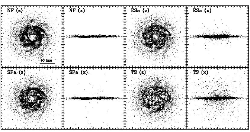
Figure 6.— Morphology of Milky Way simulations at t=323 Myr. z- and x-projections are shown to detail disk and gas halo structure. Both SPa feedback and TS lead to significant ejection of matter from the disk. ESa ‘inflates’ the disk but does not eject as much matter as TS.

The SFRs for three of the simulations (NF,TS and ESa) are plotted in figure 7. Most noticeable is the reduction in the SFR produced by TS and ESa (TS is 35% lower than no feedback at t=500 Myr, ESa is 10% lower). This is due to three factors; (a) the ejection of matter from the disk depletes the cold gas available for star formation (see figure 6), (b) smoothing feedback energy leads to spatially extended ‘puffy’ feedback regions in the disk, which in turn leads to a lower average density, and hence lower SFR, (c) particles in the feedback regions will typically be above the temperature threshold, which prevents star formation which further reduces the SFR. For single particle feedback the lower mass loss rate leads to a higher SFR than for the TS or ESa runs. Of the versions not plotted, ESna resembles the no feedback run (SFR approximately 3-4% lower on average), since most of the energy is rapidly radiated away. SPna resembles the SPa since the feedback events produce very similar effects (see section 3.3.1).

To calculate radial profiles of the disks, an arbitrary plane of thickness 6 kpc was centered on the disk. This thickness ensured that the stellar bulge was contained within the band. Radial binning was then performed on this data set using cylindrical bins.

In figure 8, gas rotation curves are compared for the simulations at t=323 Myr. To provide a fairly accurate depiction of the rotation curve that would be measured the rotation curve was calculated by radial averaging $|{\bf r}\times{\bf v}|/|{\bf r}|$ rather than by calculating the circular velocity from $\sqrt{GM(<R)/R}$. The main drawback of this method is that in the core regions, where there are few particles in the bins, the measurement can become ‘noisy’. Clearly, figure 8 shows that there is little difference between schemes (a maximum of 9% at 4 scale lengthsignoring the

Fig. 7.—SFRs for the Milky Way prototype (time-averaged over 160 time-steps to show trend). The SP variants are not shown since their evolution is similar to that of the ES version plotted. TS produces a significant (35% at t=500 Myr) reduction in the SFR as compared to no feedback. ES also reduces the SFR, but has a less significant effect (10% reduction at t=500 Myr versus no feedback) than TS.

under-sampled central values). At large radii the curves match precisely since there are no feedback events in the low-density outer regions of the disk, except for the TS run where a feedback event has ejected particles to the outer regions. Comparing to the initial rotation curve (not shown), the disk has clearly relaxed, extending both in the tail and toward the center. The curves were also examined at t=507 Myr (for those simulations integrated that long) and similar results were found with maximum differences being in the 10% range.

A more telling characteristic is the gas radial velocity dispersion. Unfortunately it is difficult to relate the measurements made here to those of molecular clouds (Malhotra (1995)), primarily because the mass scales are significantly different. Nonetheless, it is interesting to compare each of the separate feedback schemes. In figure 8 the radial velocity dispersion, $\sigma_{r}$, is plotted for three of the simulations at t=323 Myr (again only considering matter within the 6 kpc band). Temperature smoothing produces a large amount of dispersion due to the excessive energy input (interior to 8 scale lengths it varies between being 40% to 300% higher than other values). Note that there is a direct correlation between a higher velocity dispersion and a lowered measured rotation curve. This is asymmetric drift: feedback events produce velocity dispersion which in turn increases the relative drift speed, $v_{a}$, between the gas and the local circular velocity (Binney & Tremaine (1987)). The remaining algorithms (SPa, SPna, ESa, ESna) exhibit similar velocity dispersions. Thus, for all but the TS algorithm, the bulk dynamics remain the most important factor in determining the velocity dispersion. Although the velocity dispersion presented here is not directly compatible with that of the value for local molecular clouds, it is interesting to note that measurements for the Milky Way suggest $\sigma_{v_{cloud}}=9\pm 1$ km s^-1(Malhotra (1995)).

Due to the finite size of the computational grid, the code was unable to follow all of the simulations to the desired final epoch (500 Myr). This limitation was most noticeable in the SP simulations where ejected gas particles reached the edge of the computational domain within 320 Myr. It is possible to remove these particles from the simulation since they are comparatively unimportant to the remainder of the simulation. However maintaining an accurate integration was considered to be more important.

Fig. 8.—Rotation curves and radial velocity dispersions for the Milky Way prototype at t=323 Myr, for the NF, SPa, ESa and TS runs. There is only a marginal difference between rotation curves because the radial averaging smooths out the effect of inhomogeneous feedback regions. The TS gas exhibits a 8% reduction in the rotation curve at a radius of 4.5 scale lengths due to asymmetric drift. The ESa rotation curve is reduced by only 4% at this radius. The TS algorithm exhibits significantly higher velocity dispersion than any of the other variants. This is attributable to the large energy input driving winds that strongly affect the disk structure (visible in figure 6 as large holes in the disk). All the other algorithms differ only very marginally.

4.1.3 Summary

Temperature smoothing (TS) is clearly the most violent feedback method, producing an SFR lower than the other algorithms and also tending to evaporate the disk. Given the comparatively large escape velocity of the Milky Way (lower limit of 500 km s^-1 at the solar radius), this is an unrealistic model because such dramatic losses are expected only in dwarf systems. Of the remaining algorithms, the single particle (SP) versions produce reasonable physical characteristics, but have the disadvantage of requiring a large number of time-steps. The energy smoothing variant with an adiabatic period (ESa) appears to be the best compromise in these simulations. It does not require an excessive number of time-steps while the disk morphology and evolution are within reasonable bounds: there is no excessive blow-out or blow-away.

4.2. Dwarf prototype

The second model is an idealized version of NGC 6503. Dwarf systems are expected to be more sensitive to feedback due to their low mass, and consequently lower escape velocity. In simulations, the over-cooling problem suggests that to form a large disk system from the merger of small dwarfs, the dwarf systems must have significant extent (ideally similar to that for an adiabatic system, Weil, Eke & Efstathiou (1998)). Feedback is currently believed to be the best method for achieving this. Given that for NGC 6503 $v_{c}\simeq 110$ km s^-1  a lower bound on the escape velocity of the system is 155 km s^-1.

Detailed numerical studies of NGC 6503 have been conducted by Bottema and Gerritsen (1997) and Gerritsen (1997). The motivation in this investigation is different to the previous ones which attempted to explain the observed dynamics of NGC 6503. In contrast, this investigation attempts to determine bulk properties at comparatively low resolution, in accordance with that found in cosmological simulations.

4.2.1 Model Parameters

As for the Milky Way prototype, this model contains stars, gas and dark matter, with the total masses of $3\times 10^{9}$ M_⊙, $1\times 10^{9}$ M_⊙, and $5\times 10^{10}$ M_⊙ respectively. 10240 particles were used in each sector, yielding individual particle masses of $3\times 10^{5}$ M_⊙, $1\times 10^{5}$ M_⊙, and $5\times 10^{6}$ M_⊙, respectively. The radial scale length of the simulation was 1.16 kpc, and the scale height 0.1 kpc. Gas density and particle velocities were assigned in the same fashion as the Milky Way prototype. The artificial viscosity was not shear-corrected for the same reasons as the Milky Way protoype.

Six simulations were run, each using a different method of feedback (including no feedback as the control experiment). The method used in each simulation and the number of time-steps per 100 Myr are summarized in table 2.

4.2.2 Results

As in the Milky Way simulations, the SP feedback models produced significant blow-away at the outset of the simulation and particles ejected from the disk rapidly escaped from the halo. Consequently, the evolution of these systems had to be halted at very early times (close to 200 Myr). Of the remaining algorithms, only TS was not integrated to at least 500 Myr. Thus, the following analysis concentrates on the ES variants.

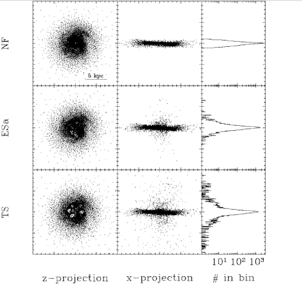
Figure 9.— Selected morphologies for the NGC 6503 model. The left hand hand column shows the z-projection of gas particles in the NGC 6503 simulation, the central column shows the x-projection and the right column displays the z-coordinate of the gas particles in the NGC 6503 simulation in bins of width 0.150 kpc ($h_{min}/2$). A significant amount of relaxation is visible in the no feedback run, with the disk fattening to a width of $\simeq 600pc$. Feedback in the TS and ESa runs ejects particles into the halo and populates the tails of the z-distribution of particles.

Figure 9 shows the distribution of gas particles in the x- and z-projections and also the z-distribution measured vertically in bins, at t=230 Myr (note that although sufficient time has elapsed for feedback events to occur the disks still exhibit virtually identical rotation curves). Due to the comparatively long softening (300 kpc) length used in the simulation, there is a significant amount of relaxation from the initially ‘thin’ distribution, which is approximately 250 pc wide. Since in the simulation code the SPH resolution is at least twice the gravitational softening length, the disk was expected to fatten to 600 pc. Figure 9 shows that this is observed (in the run with no feedback). Once feedback is included, and matter is ejected from the disk, the z-distributions develop populated tails due to particles orbiting high in the potential well. The most severe example of this being the TS variant, which rapidly ejects particles leading to significant mass loss from the disk (both blow-away and blow-out occur). The TS algorithm produces extremely large bubbles in the disk. One bubble had a radius of almost 0.7 kpc, which is 60% of the disk scale length, while for the Milky Way prototype larger bubbles had a radius of about 0.8 kpc, approximately 40% of the scale length. The absolute size of these bubbles relative to the disk is set by the SPH smoothing scale and hence should not be overinterpreted. However, the comparison of the dwarf versus the Milky Way model is valid since the particle resolution is approximately the same for both models. A comparison of the gas distributions for the ESa runs (dwarf vs. Milky Way) at 500 Myr shows that while in the dwarf system the gas density puffs up beyond the stellar component, it does not do this for the Milky Way prototype. As in the Milky Way runs, ES preferentially leads to blow-out, although by 500 Myr some particles were close to escaping the halo. These results show that feedback has a more significant effect on the dwarf system.

To calculate radial profiles of the disks a plane of thickness 2 kpc was used, centered on the disk. As for the Milky Way prototype, the thickness was chosen to ensure that the stellar content was included within the band. The data were again binned using concentric cylinders. At t=580 Myr the gas rotation curves for ESna, ESa and no feedback remain very similar (figure 10). Both of the curves exhibit asymmetric drift relative to the run with no feedback. The maximum difference (external to a radius of one scale length) occurs at 1.6 scale lengths where the adiabatic variant has a rotation curve that is 10% lower than the no feedback run. At this radius the non-adiabatic run is only 3% lower than the run with no feedback. The outer edges of the distributions remain identical due to there being no feedback events in the low-density gas.

The gas radial velocity dispersion plot (figure 10) shows that for this system ESa clearly introduces more dispersion (30% higher at a radius of 1.6 scale lengths). This is as expected: the combination of a lower escape velocity and comparatively long persistence of the feedback regions in the adiabatic variant allow the gas to escape to higher regions of the potential well. Additionally, bubble expansion in the plane of the disk persists for longer in the adiabatic variant. Notably, the run with no feedback shows an increasing velocity dispersion with radius. This can be attributed to the large softening length used, which in turn causes the SPH to smooth over a very large number of particles in the central regions (in excess of $10N_{smooth}$). Thus, in this region the gas distribution is dynamically cold.

Figure 11 shows the time-averaged SFRs for the three runs. By t=580 Myr the non-adiabatic run had ejected 1% of its mass from the disk (relative to the remaining gas), whilst the adiabatic run had ejected 2%. Examination of the raw data shows that the strongest bursting is actually found in the no feedback run. The feedback in the other two runs keeps the disk more stable against local collapse. Of the data not plotted, TS was similar to the ESa run, and had an SFR approximately 5% lower. By t=240 Myr, 6% of the disk had been evaporated. Neither of the SP runs was integrated far enough to detect

Fig. 10.—Comparison of rotation curves and radial velocity dispersions for the NGC 6503 dwarf simulation at t=580 Myr. There is little difference among all rotation curves, except in the nuclear region where feedback is more prevalent. Asymmetric drift is visible in the gas, with the ESa run having a lower rotation curve due to its higher velocity dispersion.

Fig. 11.—SFRs for the dwarf prototype. The ES and no feedback runs are shown since the remainder were not integrated for a sufficient time for conclusions to be drawn. The NF, ESa, and ESna runs were time-averaged over 320 time-steps to elucidate the trend in the SFR and this is indicated by the bar symbol in the legend. Clearly the ESa run produces the lowest SFR, being approximately 20% lower than the non-adiabatic run.

significant trends.

4.2.3 Summary

Although it was not possible to integrate all the models to the desired final epoch, it was still clearly demonstrated that feedback does have a more significant impact on the dwarf system. This is evident both in the morphology (larger relative bubbles as compared the Milky Way prototype) and radial characteristics (the radial velocity dispersion is far higher relative to the no feedback run). This increased sensitivity also allows differentiation between the adiabatic and non-adiabatic methods, which was at times difficult in the Milky Way prototype. Whether these conclusions can carry over to cosmological simulation is addressed in the next section.

5. Cosmological simulations

As discussed in the introduction, there are a number of problems that plague cosmological simulations of galaxy formation. This section examines the conjecture that, following an initial burst of star formation, feedback should be able to (1) prevent the overcooling catastrophe by suppressing massive early star formation and (2) prevent the angular momentum catastrophe, thereby allowing the formation of disks with specific angular momenta in agreement with observations. We study all of the feedback algorithms analysed in the previous sections and also include two new versions derived from combinations of the previously studied algorithms. Note that the SPH resolution ($\sim 2\times 10^{3}$ particles) in the galaxies formed in the following simulations is insufficient to resolve shocks adequately. The purpose of the simulations is to explore the parameter space and not make precise predictions about resulting galaxies. A higher resolution simulation, meeting the accuracy criteria outlined in Steinmetz & Muller (1993), will be presented in a subsequent paper.

5.1. Initial conditions

In the SPH method, shocks are captured using an artificial viscosity. The artificial viscosity is turned on or off by the value of the ${\bf r}.{\bf v}$ product between each pair of particles. The angular part of this product takes a maximal value if r and v are aligned, as is the case in collapse along a Cartesian grid. Collapse along a direction not aligned along the grid leads to scatter in the ${\bf r}.{\bf v}$ dot product, and hence less shocking. Consequently, we believe that it is advantageous to use a set of initial conditions must be used that contains no preferred direction. ‘Glass-like’ initial conditions are used in this study.

Given a hierarchical clustering scenario the first objects to form will have hundreds (at most) particles in them. Hence it is only necessary to create initial conditions which have no preferred direction on scales of the order 500 particles. The merging of the first generation progenitors occurs over scales significantly larger than a grid spacing, thus removing concerns about a preferred collapse direction for these objects. It thus makes sense to create a small periodic glass with very low noise and then tile this within the simulation box.

To create the glass ‘tile’, 512 particles are placed in a periodic box. These particles are forced to be anti-correlated by not allowing any two particles to be closer than $0.9\times N^{1/3}$, which is 0.9 times the average inter-particle spacing. This initial condition has a very low noise level. The noise level is further reduced by evolving the glass in a (periodic) gravity-only simulation with the sign of the velocity update reversed. With this modification, the particles repel one another, and eventually relax

Fig. 12.—Layering of cosmological initial conditions. Starting clockwise from the upper left panel, the top level configuration of $32^{3}$ particles is repeatedly cut and shrunk to create a hierarchy four levels deep. Gas particles are included in the central region only.

to a state in which the (repulsive) potential energy is reduced to a minimum.

Once the tile is fully evolved, it is replicated a number of times to form the main simulation cube. This configuration does not have any noise on scales larger than the size of tile and thus constitutes an excellent initial configuration. Because long-range tidal forces have a significant effect on the evolution of galaxies (Kofman & Pogosyan (1995)) they must be included in simulations. Unfortunately, a fixed resolution periodic box with equal number of dark matter and gas particles would require a prohibitively large number of particles. Hence we used the multiple mass technique (Porter (1985)) to overcome this problem. The hierarchical layers are constructed by successively cutting out a region of the simulation cube and replacing it with a copy of the top-level ‘grid’ cut and shrunk to the appropriate size. The first layer, for example, is constructed by removing a sphere of radius $1/4$ the box size and then filling that region with a sphere cut from the main simulation cube and shrunk to size. The next layer is formed by cutting a sphere of radius $1/8$ the box and replacing this with a similarly cut and shrunk sphere from the main simulation cube.

Unfortunately this process does introduce some noise at the boundary of each region. It was thus assured that in the highest resolution region, objects of interest form sufficiently far away from the boundary with the next region. The layering process continues through four layers. To maintain mass resolution, the particles in each layer have mass $1/8$ that of the previous layer. Thus the mass resolution of this region is 512 times higher than the lowest resolution region, and the spatial resolution is eight times higher. Figure 12 shows the layering in detail. If a grid of $32^{3}$ particles is initially used to perform the layering, the resulting system has 77,813 dark matter particles and 17,165 SPH particles. In the high resolution region the effective resolution is $2\times 256^{3}$.

Assigning the perturbations associated with the initial power spectrum is more difficult for multiple mass simulations. The particle Nyquist frequency is not constant across the simulation. If the box is loaded with modes up to Nyquist frequency of the highest resolution region, then aliasing of the extra modes will occur in the low resolution region. Hence, to prevent aliasing, the lower resolution regions must have their displacements evaluated from a force grid that is calculated using only modes up to the local particle Nyquist. Thus all of the box modes are calculated, and then modes are progressively removed by applying a top-hat filter in k-space.

5.2. Simulation Parameters

To assign adiabatic gravitational perturbations, the linear CDM power spectrum of Bond and Efstathiou (1984) was utilized,

$$P(k)={Aq\over[1+(23.1q+(11.4q)^{3/2}+(6.5q)^{2})^{5/4}]^{8/5}},$$ (8)

where,

$$q=k/(\Gamma h).$$ (9)

Given a baryon fraction of 10% the shape parameter, $\Gamma$, was calculated from Vianna and Liddle (1996) yielding $\Gamma\simeq 0.41$. The Hubble constant was set at 50 km s^-1 Mpc^-1, yielding in $h=0.5$ in the standard H₀=$100h$ km s^-1 Mpc^-1 units. The normalization constant, $A$, was chosen so as to reproduce the number density of rich clusters as observed today, which is given by the rms mass variance $\sigma_{8}=0.6$ (Eke, Cole & Frenk (1996)). The initial redshift was $z=67$ and the box size 50 Mpc (all length scales are quoted in real units).

Figure 13.— SFRs for the cosmological simulations. The SFR shown is integrated over the entire gas sector of the simulation ($8\times 10^{11}$ $\rm\thinspace M_{\odot}$). A 160 time-step average is used to smooth the data and more clearly elucidate trends. The effect of the smoothing is demonstrated in the no feedback panel. For comparison, the smoothed NF SFR is plotted as a dotted line in the remainder of the panels.

To ensure the collisionless nature of the dark matter does not become contaminated by two-body forces, the two-body relaxation should be longer than the Hubble time. Thomas and Couchman (1992) show that for a uniform distribution of particles (of mass m, and softening $\epsilon$) within a spherical volume of radius $R$ and with a velocity dispersion $v^{2}\sim\gamma GmN/R$ ($\gamma$ is a constant dependent upon the characteristics of the velocity distribution) the two-body relaxation time is

$$t_{r}\simeq{\gamma^{3/2}N^{1/2}\over 6\ln(R/\epsilon)}\left({R\over\epsilon}\right)^{3/2}t_{2},$$ (10)

where $t_{2}=(\epsilon^{3}/Gm)^{1/2}$ is the minimum time-scale for interactions of particles under gravity, with an effective impact parameter $\epsilon$. Utilising the velocity dispersion for an isothermal sphere and modifying the $t_{2}$ parameterization of TC92, equation 10 may be rearranged to give

$${t_{r}\over t_{0}}\simeq 0.02{(R/\epsilon)^{3/2}\over ln(R/\epsilon)}N^{1/2}\left({\epsilon\over 4{\rm\;kpc}}{50{\rm\;Mpc}\over box}\right)^{3/2}\left({N_{p}^{eff}\over 256^{3}\Omega_{p}}\right)^{1/2}.$$ (11)

Ideally the ratio $t_{r}/t_{0}$ should be greater than one, although since the simulation evolves to $z=1$, values of $0.5$ should be acceptable. The formula is minimized when $R={\rm e}^{1/2}\epsilon$ (i.e. close to the softening), and at this radius it is found that $t_{r}/t_{0}\simeq 0.08N^{1/2}$. This implies that within the softening volume, $N>10$ is neccesary to avoid two-body relaxation, although if the simulations were integrated to $z=0$, the criterion would be $N>30$.

The effective resolution of the high resolution region (which is 6.25 Mpc in diameter) is $256^{3}$, which yields a mass resolution of $4.6\times 10^{8}$ $\rm\thinspace M_{\odot}$ in the dark matter, $5.1\times 10^{7}$ $\rm\thinspace M_{\odot}$ in the gas (reducing to $2.6\times 10^{7}$ $\rm\thinspace M_{\odot}$ after the creation of the first star particle) and $2.6\times 10^{7}$ $\rm\thinspace M_{\odot}$ in the star particles. Clearly the mass resolution remains low, with a $10^{11}$ $\rm\thinspace M_{\odot}$ galaxy (in baryons) being represented by approximately 4,000 gas and star particles, assuming an equal division of both. Nonetheless, this resolution is sufficient to give a reasonable indication of the performance of different algorithms in a cosmological environment. The total baryonic mass in the high resolution region is approximately $8\times 10^{11}$ $\rm\thinspace M_{\odot}$. This is a consequence of attempting to keep the boundary of the second mass hierarchy a sufficiently long way from the object of interest, and choosing a sufficiently large box size to provide a reasonable representation of tidal forces. Since the simulated disk will was evolved over 3 Gyr, and the simulation had comparatively low resolution, shear-correction was applied to the artificial viscosity.

The first simulation conducted was a low resolution $128^{3}$ dark matter simulation using the parameters given. From this simulation, candidate halos for re-simulation were extracted at a redshift of $z=1$. Due to wall-clock limits on simulation time, it was decided that $z=1$ was the most appropriate time to stop the simulation. Whilst the dark matter run could have be continued to $z=0$, this is prohibitively expensive for the high resolution hydrodynamic runs, since it requires close to 15,000 time-steps. The chosen halo had a mass of $2.7\times 10^{12}$ $\rm\thinspace M_{\odot}$ and is thus comparatively large. Re-simulation showed that it corresponds to the halo of a merger event of two galaxies with a combined bayonic mass of $1.8\times 10^{11}$ $\rm\thinspace M_{\odot}$.

Run	feedbacka	$R_{200}$	$\Sigma m_{*}$	$|L_{gc}|/|L_{dm}|$	$M_{\rm disk}$	$R_{disk}^{\rm b}$	$R_{inner}^{\rm c}$	$R_{outer}$
		(kpc)	($10^{10}$ $\rm\thinspace M_{\odot}$)		($10^{11}$ $\rm\thinspace M_{\odot}$)	(kpc)	(kpc)	(kpc)
6001	SPa	187	$7.98$	0.25	$1.07$	8.8	1.0	34
6002	SPna	187	$8.44$	0.24	$1.14$	7.6	0.7	30
6003	ESa	188	$9.51$	0.09	$1.38$	8.0	0.6	17
6004	ESna	188	$9.38$	0.18	$1.42$	11.3†	0.7	24
6005	TSna	189	$7.45$	0.19	$1.35$	9.3	0.8	27
6006	TSa	188	$7.25$	0.27	$1.27$	9.3	0.9	24
6007	NF	189	$9.67$	0.16	$1.57$	9.5	0.9	34
6008	NSF	188	N/A	0.14	$1.29$	9.3	0.6	28
6010	TS	188	$8.69$	0.19	$1.38$	9.7	0.6	21
6014	ESa-SG	189	$9.78$	0.18	$1.25$	9.6	1.1	45
6015	ESa-2c*	189	$10.9$	0.15	$1.24$	9.1	0.9	50
6016	TSa-SG-2c*	188	$6.33$	0.33	$1.06$	10.3	1.3	39
6017	ESa-SG-2c*	189	$11.6$	0.08	$1.35$	9.2	0.8	36
6018	ESa-nav	188	$3.83$	0.23	$1.34$	8.2	0.9	36

Table 3Summary of the properties of cosmological simulations at z=1.09. ^aSPa=Single particle adiabatic period, SPna=single particle no adiabatic period but adjusted cooling density, ESna=Total energy smoothing with adjusted cooling density but no adiabatic period, ESa=Total energy smoothing with adiabatic period, TS=Temperature smoothing (normal cooling). ^bThe disk radius was evaluated by finding the radius at which the baryon surface density fell below $2\times 10^{13}$ $\rm\thinspace M_{\odot}$ Mpc^-2. This value was established by visually judging the edge of the NSF disk and then reading off the surface density at this boundary. ^cThe inner values are distorted to shorter scale lengths by the presence, or lack of, a central core in the disk. The outer fits are strongly affected by companion systems inside $r_{200}$ and strong emphasis should not be placed on these results. ^†This value is anomalously high due to a minor merger during which the stellar content of the merging dwarf orbits out at $>10$ kpc.

5.3. System evolution without feedback

Without feedback, the system follows the ubiquitous cooling catastrophe picture. Baryons condense in the halos and rapidly radiatively cool due to their high density. A disk galaxy is formed in the center of the high resolution region, with a (baryonic) mass of $1.2\times 10^{10}$ $\rm\thinspace M_{\odot}$. The disk exhibits a (visibly striking) cutoff in particle density at a radius of 8 kpc, and similarly, the vertical distribution of the disk falls off abruptly above and below 1.5 kpc of the equator. A double exponential fit of the gas density profile (see section 5.6) clearly displays the rapid fall-off in density with radius beyond 8 kpc. Star formation proceeds rapidly due to the high density, and is initially concentrated in the nucleus of the disk (which contains 40% of the baryonic mass and has a 0.6 kpc diametermuch smaller than the softening length). Stars formed in the nucleus diffuse away from it, forming a stellar bulge approximately 3.0 kpc in diameter (compare the radial density profiles in figure 15). Due to the low resolution, the hierarchical formation of the disk is represented poorly, with only a handful of progenitors merging to form the disk.

At late times $z=1.09$, the disk exhibits a number of features that have been observed previously. There is a deficit in angular momentum, with the specific angular momentum of the baryons corresponding to that of an elliptical system for the given mass scale. Consequently the disk has a small radial extent. At $z=1.01$ the disk undergoes a major merger with another system of mass $6\times 10^{10}$ $\rm\thinspace M_{\odot}$ (in baryons) at a speed of 300 km s^-1  relative to the center of mass frame for the major disk. As is generally observed in simulations with stellar and gaseous components, the resulting morphologies of the gas and stars differ significantly. The gas cores merge, creating a very dense core while the stellar components merge, producing ‘shells’ as observed in ellipitical galaxies (Quinn 1984). A tidal tail is also produced during the merger and is populated by both gas and stars.

5.4. Star Formation Rate

Unfortunately, even though the SFR normalization was adjusted to 0.025, the SFR in the simulations appears to be somewhat low. Although the plots in figure 13 show SFRs in excess of 70 $\rm\thinspace M_{\odot}$yr^-1, it should be noted that this value is integrated over $8\times 10^{11}$ $\rm\thinspace M_{\odot}$. Diagnostics from the simulation indicate that of this mass, $6.5-7\times 10^{11}$ $\rm\thinspace M_{\odot}$ is not involved in star formation ($T>30000$ K or $\rho<\rho_{sf}$). Beyond the main disk and the merger companion (a combined baryonic mass of $1.8\times 10^{11}$ $\rm\thinspace M_{\odot}$ of which 60% is in star forming regions), tertiary halos contribute only $2.4\times 10^{10}$ $\rm\thinspace M_{\odot}$ of star forming matter. Hence, the bulk of the SFR is derived from the main disk and its major companion. It should be emphasized that the halo correspondence between simulations is not perfect, but given the difficulty in accurately calculating the cooling rates at low resolution, and the highly non-linear nature of the dynamics, this is not surprising. Well-defined halos, i.e. those formed with 500 or more particles, do correspond well, as can be seen in the radial plot in figure 19. There are also small synchronization errors ($10^{5}$ years) between the analysed time-step outputs. To examine the effect of changing parameters a number of auxiliary simulations were run, the details of which are discussed in section 5.8.

5.5. Effect of feedback on SFR and morphology

The most noticeable difference in the ensemble is that the temperature smoothing version does not lead to a significantly different final structure. This is contradictory to the isolated results where temperature smoothing is seen to promote violent winds and disk disruption. The reason for this is that the density of the first objects is so high,

Fig. 14.—Radial temperature profile for the NF, SPa and ESa runs. The error bars denote 1$\sigma$ variation about the bin mean, with the data plotted in Lagrangian bins of size 208 particles. The SPa and SPna (not shown) profiles both exhibit a higher temperature at large radii (see text). Of the remaining algorithms, all follow profiles similar to the ESa and NF simulations.

$n_{H}>1\;{\rm{cm}}^{-3}$, that the cooling time ($\simeq 0.1$ Myr) is short enough to remove the SN energy within a time-step, unlike the isolated simulation where the resolution is high enough to allow a reduction in density due to expansion of the feedback region and consequent reduction in the cooling time. To test what happens when the feedback energy is allowed to persist, the TS simulations were run with the adjusted cooling mechanisms. As expected, these simulations produced more diffuse structures.

At z=1.09, the morphology of the major disk was examined. Without exception, all the simulations produced a disk with a clearly defined cutoff radius of $9.2^{+2.1}_{-1.6}$ kpc ($>2h_{min}$). This result is the same as the NF run. However, models including feedback were fatter at the disk edge, (the TSa run with a thickness of 5 kpc, being 30% wider than the NSF run). ‘Bubbles’ were noticeable in the disks, more so in the ESa run than others because the TSa and TSna runs were already quite diffuse. Feedback did not change the radial extent of the disk which suggests that it must be determined largely by the dark matter potential. It cannot be due to the central concentration of baryons, since the TSa and TSna runs effectively destroy this concentration yet still have approximately the same radius.

While the internal structure of the major disk was not significantly different across all simulations, that of the merged system was. For the NF simulation, the gaseous cores were much more tightly bound than those in the TSa and TSna runs, but were largely similar to those in the ESa, Esna, SPa and SPna runs. In particular, because the gas cores are sufficiently inflated in the TSa and TSna runs, the gas undergoes a smooth merger, and for the TSa run the feedback is sufficient to produce a disk as the result of the merger. Note that the stellar components evolve in a similar fashion though, producing shells, and a widely dispersed final stellar structure.

The SFRs for the main simulations are plotted in figure 13. The upper left panel shows the results for the simulation without feedback, and gives an illustration of the smoothing effect of the 160 step running average used to smooth the data. All algorithms agree on the early SFR, which reaches 1 $\rm\thinspace M_{\odot}\;{\rm yr}^{-1}$ at $z=3.9$, since sufficient time must pass for the star mass of particles in the highest density regions to reach the mass threshold for creating a star particle (the first star particles are created at $z\simeq 3$). At late times, the merger causes a strong star burst which is visible in all of the SFRs, albeit somewhat suppressed in the simulations with strong feedback. The relative effect of the different feedback algorithms was compared by calculating the reduction in the cumulative mass of stars at $z=1.09$, as a percentage relative to the no feedback run (total $9.7\times 10^{10}$ $\rm\thinspace M_{\odot}$). The algorithms with the most significant effects are, in order, TSa (25%),TSna (23%), SPa (18%) SPna (13%) and TS (10%) while the energy smoothing variants ESna (3%), ESa (2%) have comparatively little effect on the SFR. At earlier, epochs, in particular shortly after $z=2$, both the TS and SP runs have a significantly higher reduction in the SFR. For example at $z=1.6$ the SPna run has an SFR only 20% of the NF run. As in the isolated simulations, the SP algorithms eject particles due to asymmetry in the local distribution of particles and the subsequent reduction in the gas density is the main source of the SFR reduction over the energy smoothing variants.

5.6. Halo profiles

In view of the results from the isolated simulations, the halo structure was examined to see if there was any difference between algorithms. Figure 14 compares the gas halo temperature for the NF, ESa and SPa runs. The higher temperature seen at the edge of the SP profile (beyond 200 pc), is difficult to attribute just to ‘hot’ particles being ejected to that radii. Tracing the orbits of a number of ejected particles showed that the largest distance they achieve from the core is 150 kpc. It is noticeable that at a radius of 150 kpc, the temperature of the SP feedback halos is higher than that of the others. A plot of the radial pressure showed that beyond 200 kpc, the pressure in the SP halos is a factor of two higher than in the other runs. A plot of the cumulative density versus radius confirms that more of the gas lies at large radii (beyond 200 kpc) for the SP feedback. This indicates that the particles ejected from the disc by SP feedback are acting like a piston on the outer regions of the gas halo, subsequently leading to higher temperatures in the infalling matter at large radii (since the gravitational compression remains dominated by the dark matter).

The density profiles for the baryons can be fit by a double exponential, with the break between the two profiles occurring at the edge of the disk. An argument can be made that the presence of the gas/stellar core suggests that the disk should also exhibit a double profile; however the structure is sub-resolution. In particular, when the smoothed density is examined (which is used in the SFR calculation), there is very little difference between simulations. A summary of least squares fits for the inner and outer parts of the density profiles is given in table 3. The fitting was somewhat arbitrary since the break between the fits is decided by eye. Note that for the TS

Fig. 15.—Density profile for the NF run. Spherical Lagrangian bins (52 particles) have been used to bin the star and gas data. Clearly the gas and stellar data are comparatively similar. The stellar bulge has roughly constant density and extends to a radius of 1.5 kpc, the gas nucleus extends only just beyond 0.5 kpc. The SPH density data is a radial binning of the raw SPH density values which, because of smoothing, do not increase to the exceptionally high values seen in the radially binned stars and gas. Further, it reflects the 2-dimensional density better than the spherical bins. The self-gravity line corresponds to 0.4 times the spherically binned dark matter density.

variants, this was particularly difficult since the transition from disk to halo is less clear, i.e. the density curve is smoothly decreasing as opposed to a sharp discontinuity visible in the other data sets. The inner fits, which give an effective scale length for 3-dimensional baryon distribution in and about the disk, are broadly similar and are given by $s_{L}=0.75^{+0.25}_{-0.16}$ kpc (ignoring the auxiliary simulations presented in section5.8). Note that the gas cores tend to distort the fits toward shorter scale lengths and the three-dimensional profile underestimates the scale length that would be interpreted from a surface density plot. There is a clear trend for the adiabatic feedback schemes to have longer scale lengths than the non-adiabatic versions. This is to be expected since the adiabatic feedback keeps the gas more diffuse. The outer fits are more problematical since satellites severly distort the radially averaged density profile. Given the sensitivity of the slope to these perturbations, it is difficult to draw detailed conclusions from these data.

The gas and stellar density profiles are broadly similar since the stellar disk evolves out of the gas. Star particles that are formed within the dense central gas core eventually orbit at a larger radii than the parent particle since they are not affected by the viscous forces felt by the gas. A comparison of the gas to stellar density profile is shown in figure 15. The smoothed gas density (i.e. the SPH density) is remarkably similar across all simulations indicating that the SFR should be similar (modulo the effect of feedback events). The clear rise in the density at small radii is a signal of the gas core, albeit at sub-resolution scales. For the TSa/na runs this core was removed due to

Fig. 16.—Radial velocity dispersions in the gas disk. The minimum smoothing length $h_{min}$ and disk edges are marked for clarity. In contrast to the isolated simulations, there appears to be no correlation between more violent feedback producing higher velocity dispersion. This is partially due to the fact that merging dwarfs produce a far higher velocity dispersion than feedback, and also the disks are not well resolved.

the strong feedback. For the SP runs, the ejection of particles also lowered the core mass. The ES runs were incapable of inflating the core once formed.

The density profiles for the dark matter differ little from simulation to simulation ($r_{200}$ differs across all simulations by only 1%). At least with this mass resolution, there is no evidence for feedback being capable of rearranging the dark matter structure (Navarro et al.  (1996)).

Figure 17.— Rotation cruves for the NSF, TSa, ESa and SPa runs. The solid line shows the Plummer softened rotation curve while points indicate the tangential velocity of individual particles. Circles represent gas particles and open stars stellar particles. Particles plotted lie in a band 10 degrees wide about the plane perpendicular to the angular momentum vector of the gas. More particles appear in the TSa plot since the dense stellar core is inflated while in the other plots most of these particles fall outside the selected plane (since they are contained in the dense core). The integrated rotation curves are broadly similar and the particle data differ only marginally, with more velocity dispersion being visible in the TSa run.

5.7. Rotation curves and angular momentum

Figure 17 displays the (Plummer softened) rotation curves,

$$v^{2}_{c}(r)={GMr^{2}\over(r^{2}+\epsilon^{2})^{3/2}},$$ (12)

and particle tangential velocities for the run without star formation compared to the ESa, SPa and TSa runs. For all simulations, the tangential velocities rise more sharply than the rotation curve. However, the initial slope of the rotation curve is dominated by the softening parameter and a 12% reduction in the softening length is enough to fit the tangential data, hence this should not be considered a significant discrepancy. The 300 km s^-1  peak of the rotation curve is consistent with the mass of the disk and halo, although the SPa run is slightly lower since gas has been ejected out of the disk into the halo.

The TSa run shows significantly increased dispersion in the tangential velocities because of the feedback, but does not have a larger disk diameter (in keeping with the similar scale lengths found in the analysis of the density profiles). Since particles involved in feedback regions tend to be ejected vertically from the disk, i.e. preferentially into low density regions, a large tangential velocity dispersion can arise. This is seen most clearly in the TSa plot.

In view of the rotation curves being similar across all simulations, it would be expected that the velocity dispersions should also exhibit similar profiles. A comparison plot of the NSF run compared to the SPa, TSa and TSa-SG-2c* run (note this run has double the fiducial SFR and no self-gravity criterion, see section 5.8) is shown in figure 16. As expected, the profiles are broadly similar with a maximum difference between the plotted runs of 20 km s^-1 at the disk edge. It is interesting to note that the TSa run has a large tangential velocity dispersion, as is visible in figure 17, but a comparatively low dispersion in the radial direction. This is a result of feedback preferentially ejecting particles vertically, in turn boosting the tangential velocity component more than the radial. The data for the NF run (not shown) are dominated by an ongoing merger which introduces a very large dispersion (120 km s^-1) at the edge of the disk, far larger than that produced by any feedback. The NF and ESa runs also show the effect of the merger, with peaks in the data at 4.2 kpc and 3.6 kpc respectively, corresponding to the position of the strongest perturbation within the disk. The SPa and TSa runs are less affected by the merger since the dwarf has been reduced in mass by the stronger feedback. It is clear that the low resolution in the disks and the complications of ongoing mergers make it difficult to draw conclusions from this data.

To see how much angular momentum has been lost by the disk, the specific angular momentum of the cores is compared to that of the dark matter halo (within $r_{200}$) in figure 18. The angular momentum for the halo gas (the gas for which $\delta<2000$ within $r_{200}$) and that of the stellar component of the disk are also shown. For all simulations, the disk system shows a deficit of specific angular momentum when compared with the dark matter. By breaking the disk into its stellar component and gas component, it becomes clear that in the simulations with feedback that are shown (TSa, SPa and TSa-SG-2c^∗) there is a trend toward higher angular momentum values for the gas disk. The highest value, that from the TSa-SG-2c^∗ simulation, just falls within the disk region of the parameter space. However, the stellar disks all fall in the elliptical region of the parameter space, and the effect of feedback on them is small. Note that the purely gaseous run also sits in the elliptical region and the gas disk in the no feedback run has marginally higher specific angular momentum than the stellar component. The NF run is misleading, since a merger is going on at the edge of the disk leading to higher angular momentum values as compared to the other feedback runs (although by the end of the merger the opposite

Fig. 18.—Specific angular momenta versus mass for different components of the system for a number of different feedback algorithms. The filled polygons plot the angular momentum of the dark matter within $r_{200}$, the open polygons that of halo gas (all gas that does not fall above $\delta=2000$), pointed stars that of the gas in the main disk ($\delta>2000$) and finally the centrally connected stars show that angular momentum of the stellar component of the disk. The runs with feedback show a small but noticeable trend toward higher angular momentum values for the gas disk component (contrast with the NF run). Both dark matter and gas halo values are in broad agreement as expected.

will be true due to core-halo interaction). For all simulations, the angular momentum of the halo gas is larger than that of the dark matter since the dark matter plot includes the contribution of the dark matter core, which has little angular momentum but a significant amount of mass. It is clear from the plot that if the halo gas were to fall smoothly onto the disk, then it should be possible to form a disk with an angular momentum value midway between that of the halo gas and disk system. Note infalling satellites may still disrupt the disk and cause still further angular momentum loss.

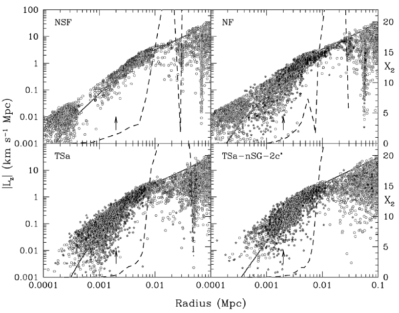
Figure 19.— Plot of specific angular momentum versus radius, showing the raw particle data versus $|L_{z}|$ calculated from the rotation curve at $z=1.09$ (counter rotating particles are not shown). The $X_{2}(R)$ stability parameters for the disks are also shown. The raw data fits the expected curve well, indicating that at least at the current epoch (prior to significant accretion) there has not been significant angular momentum loss as a result of disk formation (a bar is yet to form). The large concentration of matter at very small radii in the NF and NSF runs is the central core and is slightly offset, since the center of mass velocity was measured over the entire disk rather than the core. The $X_{2}(R)$ plots are all similar with little difference even for the extreme feedback in the TSa-SG-2c^∗ run. Disk stability occurs at $X_{2}(R)\simeq 3$ and is achieved at the smallest radius of 3.5 kpc in the NSF run and at the largest radius of 6.0 kpc for the TSa-SG-2c^∗. Note that the TSa runs provide sufficient feedback to remove the central mass concentration, but fail to increase the disk radius significantly.

The z-component of the specific angular momentum L is shown in figure 19. If significant angular momentum loss occurs as a result of disk formation then a larger proportion of the disk mass should lie beneath the line formed by $|\bf{r}\times\bf{v}_{circ}|$. Since this is not the case, it is clear that at $z=1.09$ there has been little angular momentum loss (within the disk) due to bar formation. However, all the disks are deficient in angular momentum relative to the halo, since they have been formed in a hierarchical process which is subject to core-halo angular momentum transport. Remarkably, the $X_{2}(R)$ stability parameter (Toomre (1981); Binney & Tremaine (1987)) plots are all similar, with all the disks achieving the $X_{2}(R)\simeq 3$ stability requirement just beyond the 4 kpc softening radius. As was shown by Dominguez-Teneiro et al. (1998), it is more than likely that if the baryonic mass is redistributed into an exponential disk, then the $X_{2}(R)$ parameter for this system does not achieve stability until a much larger radius, i.e. the cores provide disk stability. Note that the kink in the $X_{2}(R)$ plot for the NF run is due to the merger previously discussed and it does not affect the disk stability greatly (the kink drops to 2 at 6.5 kpc but quickly returns to stable values).

5.8. Auxiliary simulations

To adequately examine the parameter space of these simulations and also determine the effect of SPH algorithm changes would take an excessively long time. Alternatively, by conducting a few auxiliary simulations, much can be learnt about the outer edges of the parameter space. To understand what happens when the SPH algorithm is changed, in particular in relation to the treatment of high density regions, it is simple to contrast to one of the previous simulations run with the same parameters.

Figure 20.— SFRs for the auxiliary cosmological simulations. The SFR shown is integrated over the entire gas sector of the simulation ($8\times 10^{11}$ $\rm\thinspace M_{\odot}$), and time averaging is used to smooth the data. Doubling the SFR normalization does not lead to a perfect doubling of the SFR, although peak values are close. Removal of the self-gravity criterion leads to the very early onset of star formation. The TSa-SG-2c* simulation has strong feedback and even with the higher SFR normalization still has a lower peak SFR than the ESa run (plotted for comparison). The ESa-SG-2c* run, while having a peak SFR earlier, is not significantly different from the ESa run. Changing the short range behaviour of the SPH solver leads to a markedly different SFR, as shown in the plot of the ESa-nav data. The peak of the SFR is later and lower, and the self-gravity criterion only mildly delays the onset of star formation.

As indicated in previous sections, to determine the effect of removing the self-gravity criterion, the ESa simulation was rerun without it. This simulation is denoted ESa-SG. Also the effect of doubling the star formation rate normalization was tested in a simulation denoted ESa-2c*. Since most of the simulations conducted appeared to be relatively unchanged by the introduction of feedback, a simulation with extremely violent star formation and feedback was run (twice the fudicial SFR normalization with TSa feedback and also without the self-gravity criterion). This simulation, denoted TSa-SG-2c^∗, is not particularly realistic (star formation begins very early and the feedback is over-efficient) but it does provide an excellent guide to the limits of what feedback can accomplish. Because of the strong feedback, the formation of dense gas cores was all but prevented, with the exception of very large $>5\times 10^{10}$ $\rm\thinspace M_{\odot}$ systems. Hence it was possible to integrate the system to later times since the SPH algorithm did not suffer significant slow down. An ESa-SG-2c^∗ simulation was also run to contrast with the temperature smoothing version.

As an alternative to smoothing over all the particles within the minimum smoothing length, $h_{min}$, literature on galaxy formation (this appears to be implied in Navarro & White (1993); Bate & Burkert (1997)) suggests that one may continue search over $N_{smooth}$ neighbour particles. Such a procedure places a direct limit on the maximum resolved density: the volume normalization is set by $h_{min}$ and the summation over neigbours is limited to $N_{smooth}$ particles. In turn, this sets a bound on the maximum SFR per particle and consequently within the system as a whole. It also sets a bound on the cooling rate. The reasons for making this change are primarily related to efficiency: if a simulation smooths over all the particles within $h_{min}$ it can exhibit a severe slowdown. For example, nearly all the simulations without this adjustment slow down by a factor of 7 from start to finish. Hence to examine the effect of making this change, the ESa simulation was re-run with this high density treatment. This simulation is denoted ESa-nav. It is interesting to note that this method can be made to almost exactly reproduce the density values calculated in a simulation with $h_{min}\rightarrow 0$, a volume normalization is the only thing that need be applied.

In the ESa-SG run, the effect of removing the self-gravity criterion is that star formation begins at a very early epoch (1 $\rm\thinspace M_{\odot}\;{\rm yr}^{-1}$  at $z=8.3$, see figure 20). It is initially confined to a few particles (recall the $\nabla.{\bf v}$ criterion must also be fulfilled) leading to an SFR of 0.2 $\rm\thinspace M_{\odot}\;{\rm yr}^{-1}$. During later evolution, the SFR is only marginally lower than that of the ESa run, the largest difference being 10 $\rm\thinspace M_{\odot}\;{\rm yr}^{-1}$  at $z=2.1$ (a 12% difference). Further, the disk and halo structure are comparatively similar, as measured by density and temperature profiles, and the dense gas core is still formed.

The plot of the SFR in the ESa-2c^∗ simulation (figure 20) shows that doubling the SFR normalization leads to a stronger initial star burst as the gas overcomes the self-gravity criterion, but does not produce an SFR that is exactly double that of the standard simulations. The peak SFR of 120 $\rm\thinspace M_{\odot}\;{\rm yr}^{-1}$ at $z=2.1$ is 56% higher than that in the ESa run (77 $\rm\thinspace M_{\odot}\;{\rm yr}^{-1}$). The SFR is not simply doubled because of both increased feedback and the finite amount of gas available for star formation. Notably the dense gas core was still formed, showing that even with the increased SFR, ESa is still incapable of producing a significant effect on morphology.

As expected, the TSa-SG-2c^∗ simulation leads to markedly different results than any of the previous simulations. Because of the extreme feedback and consequent absence of small progenitors, the disk assembly process is very smooth. There is essentially no formation of a gas and stellar nucleus within the disk. Star formation begins at the same epoch as the ESa-SG run, albeit at a higher rate due to the increased SFR normalization which yields 1 $\rm\thinspace M_{\odot}\;{\rm yr}^{-1}$ at $z=9.1$. At $z=6.2$ the SFR reached 15 $\rm\thinspace M_{\odot}\;{\rm yr}^{-1}$ and a peak of 52 $\rm\thinspace M_{\odot}\;{\rm yr}^{-1}$ occurred at $z=3.0$. The most noticeable difference in the SFR is that at late times it falls off precipitously. At $z=1.0$ the SFR is 18 $\rm\thinspace M_{\odot}\;{\rm yr}^{-1}$ compared to 36 $\rm\thinspace M_{\odot}\;{\rm yr}^{-1}$ for the ESa run and by $z=0.5$ it had fallen to 5 $\rm\thinspace M_{\odot}\;{\rm yr}^{-1}$. Note the decay in the SFR versus time was linear rather than exponential, This has been observed before in parameter space explorations (Thacker (1997)). The less energetic feedback provided by energy smoothing leads to the ESa-SG-2c^∗ simulation producing a much higher peak SFR, namely 80 $\rm\thinspace M_{\odot}\;{\rm yr}^{-1}$ at $z=2.7$. In keeping with all the other energy smoothing simulations, a central gas nucleus was formed in the disk and the temperature and density profiles remain similar to the ESa run.

At $z=0.5$, the TSa-SG-2c^∗ disk was analysed to see if the accretion of the halo gas had indeed allowed the formation of a disk without an angular momentum deficit. By this epoch, the disk had grown to a diameter of 12.0 kpc, which is 17% larger than the value from $z=1.09$ and the mass had increased by 30% to $1.39\times 10^{11}$ $\rm\thinspace M_{\odot}$. $r_{200}$ had grown to 285 kpc. The ratio of the specific angular momenta for the gas core and dark matter, increased to 0.40 (20% increase). Visualization of the system shows that the ratio cannot increase significantly as there are very few cold gas clumps within the dark matter halo available for accretion. Most have been blown apart by feedback. Note that at the center of the halo the gas density is approximately $n_{H}\simeq 10^{-3}$ cm${}^{-}3$ and the temperature is over $10^{6}$ K, leading to a cooling time of greater than $4\times 10^{9}$ years. Hence very little of this gas, which has a large specific angular momentum, can cool on to the gas disk before $z=0$.

The results from the ESa-nav simulation are very different. The peak SFR is 38 $\rm\thinspace M_{\odot}\;{\rm yr}^{-1}$ and it occurs at a much later time than the rest of the simulations ($z=1.1$). Also star formation begins slightly later than that seen in the simulations without the self-gravity criterion (1 $\rm\thinspace M_{\odot}\;{\rm yr}^{-1}$ by $z=6.9$) which is significantly earlier than the standard simulations (1 $\rm\thinspace M_{\odot}\;{\rm yr}^{-1}$ by $z=3.9$). The reduced SFR is due to the density values calculated by this method being lower and not due to any increased effect of feedback. The change in the epoch at which the self-gravity criterion is overcome is due to the change in the search radius. In the center of the halo the dark matter profiles have a much shallower density profile than the baryon cores. When the neighbour search is conducted over the reduced radius only the core is sampled rather than the full 4 kpc radius, i.e. the sharp decline in baryon density at the disk edge is ignored. The disk formed is broadly similar to that in the ESa run, although it has a slightly larger baryon core, a thinner structure (2 kpc thick) and a smaller radius.

As was expected, the wall-clock per time-step slowdown was less severe for this code and it was roughly double the speed of the standard implementation. Note that this is an underestimate of the efficiency since the $h$-update algorithm did not accurately calculate the required change in the search radius for regions where it was less than $2h_{min}$, see Thacker et al (1998) for a full discussion. The algorithm preferentially smooths over too many particles, and an accurate calculation would require a very short time-step.

6. Summary and Discussion

This paper details a study of a number of different feedback algorithms, comparing the effect on high resolution isolated systems and low resolution hierarchical simulations. The parameter space of the model was explored as were the effects of small changes in the hydrodynamic solver.

Principal conclusions follow:

1. As would be expected on energy budget grounds, the temperature smoothing (TS) feedback algorithm has the most impact on structure formation. Single particle (SP) feedback has a less significant but still noticeable effect and it produces a distinct change in the temperature profile of the halo at large radii. Energy smoothing (ES) is the least effective of the three fundamental mechanisms.

2. Feedback can be shown to have a large effect in systems that are well resolved in terms of particle number. In particular, the Milky Way and NGC 6503 prototypes are strongly affected by feedback even though the softening lengths were chosen to be comparable with those of cosmological simulations. Both ‘blow-out’ and ‘blow-away’ can be produced, depending upon the feedback algorithm.

3. The NGC 6503 prototype is more strongly affected by feedback than the Milky Way prototype, i.e. feedback has more effect on low mass systems, as expected. In the NGC 6503 model it is possible to differentiate between the cooling mechanisms.

4. In hierarchical simulations even an excessive amount of feedback, TSa-SG-2c^∗ for example, produces little effect on the properties of large ($>10^{11}$ $\rm\thinspace M_{\odot}$) disk galaxies at early epochs. Rotation curves and density profiles remain broadly similar.

5. Although small at the mass scale probed by the hierarchical simulations, there is a distinct trend toward higher specific angular momentum values in the disk with increased feedback. At lower mass scales, equivalently at higher resolution, the effect should be more noticeable.

6. The revised cooling mechanism has little effect for the energy smoothing algorithm since insufficient energy is input, and consequently, the estimated density does not lower the cooling rate significantly. Conversely, for single particle feedback and temperature smoothing, the energy input is more than sufficient to force the cooling rate from the estimated density to be much longer than the local one.

7. Morphologies remain broadly similar in hierachical simulations although feedback can reduce the SFR, compared to runs without it, by over 25% at z=1. At earlier epochs reductions of significantly over 50% were seen. Note that the reduced SFRs continue to offer similar peaks and troughs albeit at a lower overall normalization.

8. The introduction of a self-gravity criterion to prevent catastrophic star formation at high redshifts does not lead to significantly different structure formation provided that the SFR normalisation is set within reasonable bounds.

9. The treatment of the high density end of the SPH solver can produce an enormous difference in the SFR. By reducing the neighbour search in the high-density regions the SPH density becomes lower and consequently so does the SFR. Also the self-gravity criterion is overcome earlier since as the search radius is reduced the baryonic cores have a higher weighting.

At the resolution provided by the cosmological simulations hierarchical merging is not adequately modeled. Only a handful of progenitor halos merge to form the major disk system. That all of the simulations, including those with the exceptional feedback provided by temperature smoothing, produce an over-compact disk is not cause for concernthe radius of the disk is determined largely by the depth of the potential well. Due to the early stage at which the simulations were stopped, it is difficult to comment on the evolution of the majority of disk systems, which are expected to accrete a large fraction of mass from $z\simeq 1$ onwards. The one simulation that was integrated to $z=0.5$ gave some surprising results. If feedback is sufficiently strong to reduce the angular momentum problem for the largest systems then there are insufficient halos at later times to accrete on to the disk. Although it is a significant jump to go from this result to the idea that feedback was stronger at higher redshifts it certainly seems appealing. Silk (1998) discusses variations in the IMF over time.

One particularly important area that has not been examined is the effect of resolution. For star formation algorithms based upon density values, there are many issues to be considered. In particular, in a hierarchical cosmology, star formation will be higher and begin at earlier epochs with increased resolution. The effect on feedback is less clear but by increasing the mass resolution in simulations the escape velocity of the first halos is reduced. Since the gas temperature following a feedback event is not reduced (with increased resolution), heated gas will tend to orbit higher in the potential well and be more diffuse. It was noted that in the simulations with energy smoothing (even those with a high SFR) the formation of a dense central core was unavoidable. This might be partially associated with the delay between the first star formation and the first feedback. During this time it may be the case that gas can accumulate above the mass threshold at which it can be blown out. A probablistic star formation algorithm might improve this matter somewhat, although in the limit $N\rightarrow\infty$ these algorithms should converge. However, it should be acknowledged that the dark matter halos in the sCDM picture have a strong central concentration and that the core accumulation may be a result of this.

As is widely known, core-halo angular momentum transport presents great problems for the sCDM picture. An important question is what is the extent of the problem for merging halos of unequal mass? It is unclear whether the limiting case of accreting a large number of low mass halos will lead to a system that has not lost a significant proportion of its angular momentum. Since the internal angular momentum of the final object is carried by the orbital angular momentum of the progenitors, there is reason to believe that it should be possible. However, higher resolution SPH studies (Thacker and Couchman, forthcoming) indicate that it is almost impossible to avoid the formation of large objects from mergers of smaller ones without the angular momentum problem coming in to play – there are too many ‘medium sized’ halos that collapse within the galaxy halos. It is also possible to make insights without relying upon high resolution since the power spectrum relevant to galaxy formation is the approximately scale invariant $P(k)\propto k^{-2}$ (cooling times are shorter for the smaller halos, and the power spectrum is tilted more toward $P(k)\propto k^{-3}$). The simulations thus performed give a good indication of the properties of the low mass progenitors of galaxies – they too should suffer from an angular momentum deficit. However, since this is a problem for the internal angular momentum and not the orbital, the effect on the final object may not be a significant problem. In light of this argument, it is seen that smooth infall in simulations occurs as a result of a lack of resolution. Indeed the idea of smooth infall in sCDM is largely a misnomer (at least without some kind of feedback mechanism). In simulations, the minimum mass scale effectively keeps the gas supported against the collapse that would normally ensue given higher resolution. Thus the disks that are formed in SPH simulations are a result of this lack of numerical resolution, and ideally detailed convergence studies should be undertaken. A number of authors have already hinted at this problem (Evrard et al. 1994; Weinberg, Hernquist & Katz 1997, for example), but as yet no systematic attempt has been made to deal with it or its effects. This problem is revisted in a paper in preparation.

The large variations in SFRs that may be produced by small changes in the parameter space remain a significant concern. The treatment of the high density end of the SPH solver is of particular importance, since it can strongly affect the SFR calculated, and further the treatment is not performed in the same manner by all research groups. The development of a standard test case for dynamical star formation algorithms is desireable, the facilitating the comparison of different research results. Unfortunately, it is far from clear what kind of a test case should be adopted. Simple rotating cloud collapse models are not adequate since they provide no representation of the hierarchical formation process or the effect of tidal fields. Also, since some algorithms are grid-based and some are particle-based, it may be necessary to adopt a suite of similar test cases.

McGaugh (1998) presents a survey of a number of reasons why sCDM is unable to form low surface brightness (LSB) galaxies similar to those observed. Nonetheless, it is still instructive to compare the SFRs calculated with those from deep observations of star forming galaxies. Studies of the global SFR, when adjusted for dust extinction, suggest that there is no decline between $z=1$ to 4.5. Consequently, the self-gravity criterion imposed, causing an abrupt turn on of star formation at $z=4$, does not fit the data, especially the observations of Chen et al. (1999) suggesting star formation at $z\simeq 7$. This should not be over-interpreted since it is a result of a lack of resolution, adding higher resolution would move the onset of star formation to progressively earlier times. Turning off the criterion allows star formation to proceed very early on, at $z=8.3$, but it also allows star formation to occur in regions where the dark matter may still be dynamically dominant, which is undesirable. Using the continuum UV flux, the DEEP survey of the Hubble Deep Field derives SFRs from 0.14 $\rm\thinspace M_{\odot}\;{\rm yr}^{-1}$ to 24.92 $\rm\thinspace M_{\odot}\;{\rm yr}^{-1}$ for $q_{0}=0.05$ and $q_{0}=0.5$ values are 11 times lower (Lowenthal et al (1997)). Note that these values are not corrected for dust extinction. At $z=3$ the SFRs calculated (30-70 $\rm\thinspace M_{\odot}\;{\rm yr}^{-1}$) are higher than those found, although the selected sample are categorized as “large dwarf spheroidals” and, in contrast, at $z=3$ the simulated galaxy already has a mass of $7.2\times 10^{10}$ $\rm\thinspace M_{\odot}$. More recently estimates of SFRs derived from H$\beta$ emission, for a sample of $z=3$ galaxies, have shown widely diverging values compared to the estimate from the UV flux (with both fluxes being uncorrected for dust extinction). The H$\beta$ values are larger, by as much as a factor of 7, yielding SFRs in the range 20-270 $\rm\thinspace M_{\odot}\;{\rm yr}^{-1}$ (Pettini et al.  (1998)). It is difficult to see how the models presented can be tuned to produce SFRs in the region of 270 $\rm\thinspace M_{\odot}\;{\rm yr}^{-1}$ since it would require an SFR normalization far beyond what we believe is the realistic parameter space. A forthcoming paper examines the effect of higher spatial resolution on the derived SFR.

References

- Barnes (1992) Barnes, J., 1992, ApJ, 393, 484
- Barnes & Efstathiou (1987) Barnes, J., & Efstathiou, G., 1987, ApJ, 319 575
- Bate & Burkert (1997) Bate, M.R., & Burkert, A., 1997, MNRAS, 288, 1060
- Binney & Tremaine (1987) Binney, J., & Tremaine, S., 1987, ‘Galactic Dynamics’, Princeton University Press, Princeton.
- Bond & Efstathiou (1984) Bond, J. R., & Efstathiou, G., 1984, ApJL, 285, L45
- Bottema & Gerritsen (1997) Bottema, R. & Gerritsen J. P. E., 1997, MNRAS, 290, 585
- Carlberg & Couchman (1989) Carlberg R. G. & Couchman H. M. P., ApJ, 340, 47, 1989
- Chen et al. (1999) Chen, H. W., Lanzetta, K. M., & Pascarelle, S., 1999, Nature, 398, 586
- Couchman (1991) Couchman, H. M. P., 1991, ApJL, 368, L23
- Couchman, Thomas & Pearce (1995) Couchman, H. M. P., Thomas, P. A., & Pearce, F. R., 1995, ApJ, 452, 797
- Christodoulou et al. (1995) Christodoulou, D. M., Shlosman, I., & Tohline, J. E., 1995, ApJ, 443, 551
- Dominguez-Tenreiro et al. (1998) Dominguez-Tenreiro, R., Tissera, P. B., & Saiz, A., ApJL, 508, L123
- Efstathiou (1992) Efstathiou, G., 1992, MNRAS, 256, 43
- Eke, Cole & Frenk (1996) Eke, V. R., Cole, S., Frenk, C. S., 1996, MNRAS, 282, 263
- Evrard, Summers & Davis (1994) Evrard, A. E., Summers, F. J., & Davis, M., 1994, ApJ, 422, 11
- Fall & Efstathiou (1980) Fall, S. M., Efstathiou, G., 1980, MNRAS, 193, 189
- Gerritsen & Icke (1997) Gerritsen, J. P. E., & Icke, V., 1997, A&A, 325, 972
- Gerritsen (1997) Gerritsen, J. P. E., 1997, PhD thesis, Kapetyn Astronomical Institute.
- Gingold & Monghan (1977) Gingold R. A., Monaghan, J. J., 1977, MNRAS, 181, 375
- Hernquist (1995) Hernquist, L., ApJS, 86, 389
- Hultman & Pharasyn (1999) Hultman, J., & Pharasyn, A., 1999, A&A, 347, 769
- Katz (1992) Katz, N., 1992, ApJ, 391, 502
- Kennicutt (1998) Kennicutt, R. C., 1998, ApJ, 498, 541
- Kofman & Pogosyan (1995) Kofman, L., & Pogosyan, D., 1995, ApJ, 442, 30
- Lowenthal et al (1997) Lowenthal, J. D., Koo, D. C., Guzman, R., Gallego, J., Phillips, A. C., Faber, S. M., Vogt, N. P., Illingworth, G. D., & Gronwall, C., 1997, ApJ, 481, 673
- Lucy (1977) Lucy, L. B., 1977, AJ, 82, 1013
- Malhotra (1995) Malhotra, S., 1995, ApJ, 138, 448
- Martel & Shapiro (1998) Martel, H., & Shapiro, P. R., 1998, in 19th Texas Symposium on Relativistic Astrophysics and Cosmology, eds, J. Paul, T. Montmerle and E. Aubourg, CEA Saclay, Paris.
- McGaugh (1998) McGaugh, S., 1998, in ‘Galaxy Dynamics’ conference held at Rutgers University, eds D. R. Merritt, M. Valluri & J. A. Sellwood, ASP Conference Series, San Francisco.
- Mckee & Ostriker (1977) Mckee C. F., & Ostriker J. P., 1977, ApJ, 218, 148
- Mihos & Hernquist (1994) Mihos, J. C., & Hernquist, L., 1994, ApJ, 437, 611
- Navarro & Steinmetz (1997) Navarro, J. F., & Steinmetz, M., 1997, ApJ, 478, 13
- Navarro et al. (1996) Navarro, J. F., Eke, V. R., & Frenk, C. S., 1996, MNRAS, 283, L72
- Navarro et al. (1995) Navarro, J. F., Frenk, C. S., & White, S. D. M., 1995, MNRAS, 275, 56
- Navarro & White (1993) Navarro J., & White S. D. M., 1993, MNRAS, 265, 271
- Navarro & White (1994) Navarro J., & White S. D. M., 1994, MNRAS, 267, 401
- McKee & Ostriker (1977) McKee, C. F., & Ostriker, J. P., 1977, ApJ, 218, 148
- Pebbles (1980) Peebles, P. J. E., 1980, The Large-Scale Structure of the Universe (Princeton: Princeton Univ. Press).
- Pettini et al. (1998) Pettini, M., Kellogg, M., Steidel, C. C., Dickinson, M., Adelberger, K. L., & Giavalisco, M., 1998, ApJ, 508, 539
- Porter (1985) Porter, D., 1985, PhD Thesis, University of California at Berkeley.
- Quinn (1984) Quinn, P. J., 1984, ApJ, 279, 596
- Rees & Ostriker (1977) Rees, M. J., & Ostriker, J. P., 1977, MNRAS, 179, 541
- Silk (1998) Silk, J., in The Stellar Initial Mass Function (38th Herstmonceux Conference), ASP Conference Series, San Francisco.
- Sommer-Larsen, Gelato & Vedel (1998) Sommer-Larsen J., Gelato, S., & Vedel H., 1998, astro-ph/9801094, accepted for publication in ApJ.
- Steinmetz & Muller (1993) Steinmetz, S., & Muller, E., 1993, A&A, 268, 391
- Steinmetz & Muller (1994) Steinmetz, S., & Muller, E., 1994, A&A, 281, L97
- Steinmetz & Muller (1995) Steinmetz, S., & Muller, E., 1995, MNRAS, 276, 549
- Sutherland & Dopita (1993) Sutherland, R. S., Dopita, M. A., 1993, ApJS, 88, 253
- Toomre (1981) Toomre, A., 1981, in The Structure and Evolution of Normal Galaxies, eds. S. M. Fall & D. Lyden-Bell, (Cambridge: Cambridge Univ. Press), P. 111
- Thacker (1997) Thacker, R. J., keynote seminar, Canadian Astronomical Society meeting 1997, Edmonton, Alberta.
- Thacker et al (1998) Thacker, R. J., Pearce, F. R., Tittley, E. R., Couchman, H. M. P., & Thomas, P. A., 1998, astro-ph/9809211, submitted to MNRAS
- Thomas & Couchman (1992) Thomas, P. A., & Couchman, H. M. P., 1992, MNRAS, 257, 11
- van den Bosch (1998) Van Den Bosch, F. C., 1998, ApJ, 507, 601
- Vianna & Liddle (1996) Viana, P. T. P., Liddle, A. R., 1996, MNRAS, 281, 323
- Weil, Eke & Efstathiou (1998) Weil, M. L., Eke, V. R., & Efstathiou, G., 1998, MNRAS, 300, 773
- Weinberg et al. (1997) Weinberg, D. H., Hernquist, L., & Katz, N., 1997, ApJ, 447, 8
- White (1994) White, S. D. M., 1994, Formation and evolution of galaxies: Les Houches lectures, astro-ph/9410043.
- White & Frenk (1991) White, S. D. M., & Frenk, C. S., 1991, ApJ, 379, 52
- White & Rees (1978) White, S. D. M., & Rees, M. J., 1978, MNRAS, 183, 341
- Yepes et al (1997) Yepes, G., Kates, R., Khokhlov, A., & Klypin, A., 1997, MNRAS, 284, 235