Probing the Cosmic Dark Age in X–rays

Abstract

Empirical studies of the first generation of stars and quasars will likely become feasible within the next decade in several different wavelength bands. Microwave anisotropy experiments, such as MAP or Planck, will set constraints on the ionization history of the intergalactic medium due to these sources. In the infrared, the Next Generation Space Telescope (NGST) will directly detect sub–galactic objects at $z\;\hbox to0.0pt{\lower 2.5pt\hbox{$\sim$}\hss}\raise 1.5pt\hbox{$>$}\;10$. In the optical, data from the Hubble Deep Field (HDF) already places a constraint on the abundance of high–redshift quasars. However, the epoch of the first quasars might be first probed in X–ray bands, by instruments such as the Chandra X-ray Observatory (CXO) and the X-ray Multi-mirror Mission (XMM). In a 500 Ksec integration, CXO reaches a sensitivity of $\sim 2\times 10^{-16}~{}{\rm erg~{}s^{-1}~{}cm^{-2}}$. Based on simple hierarchical CDM models, we find that at this flux threshold $\sim 10^{2}$ quasars might be detectable from redshifts $z\;\hbox to0.0pt{\lower 2.5pt\hbox{$\sim$}\hss}\raise 1.5pt\hbox{$>$}\;5$, and $\sim 1$ quasar at $z\sim 10$, in each $17^{\prime}\times 17^{\prime}$ field. Measurement of the power spectrum of the unresolved soft X–ray background will further constrain models of faint, high–redshift quasars.

KEYWORDS: cosmology: theory; quasars: general; black hole physics

1. Introduction

The cosmic dark age ended when the first gas clouds condensed out of the primordial fluctuations at redshifts $z=10-20$ (Peacock 1992; Rees 1996). These condensations are likely the sites where the first clusters of stars and the first quasar black holes appeared, giving birth to the first “mini–galaxies” or “mini–quasars” in the Universe. Despite the lack of observational data, this epoch has become a subject of intense theoretical study in the past few years. The recent interest can be attributed to forthcoming instruments: NGST could directly image sub–galactic objects at $z\;\hbox to0.0pt{\lower 2.5pt\hbox{$\sim$}\hss}\raise 1.5pt\hbox{$>$}\;10$ in the infrared, while microwave satellites such as MAP or Planck could measure signatures from the reionization of the intergalactic medium (IGM). Currently, bright quasars are detected out to $z\sim 5$ (Fan et al. 1999). Although the abundance of optically and radio bright quasars declines at $z\;\hbox to0.0pt{\lower 2.5pt\hbox{$\sim$}\hss}\raise 1.5pt\hbox{$>$}\;2.5$ (Schmidt et al. 1995; Shaver et al. 1996), a recent determination of the X–ray luminosity function (LF) of quasars from ROSAT data (Miyaji et al. 1998a) has not confirmed this decline. In this contribution, we point out that future X–ray observations might provide yet another probe of the first quasars and the end of the dark age at $z\sim 10$, and that X–ray data might be uniquely useful in distinguishing quasars from stellar systems.

2. The Appearance of the First Quasars and Stars

In popular Cold dark matter (CDM) cosmologies,the first baryonic objects appear near the Jeans mass ($\sim 10^{6}~{}{\rm M_{\odot}}$) at redshifts as high as $z\sim 30$ (Haiman & Loeb 1999b, and references therein). At any redshift, the mass function of collapsed dark halos is given to within a factor of two by the Press–Schechter formalism. Following collapse, the gas in the first baryonic condensations is virialized by a strong shock (Bertschinger 1985). Provided it is able to cool on a timescale shorter than the Hubble time, the shock–heated gas continues to contract. Depending on the details of the cooling and angular momentum transport, the gas then either fragments into stars, or forms a central black hole exhibiting quasar activity. Although the actual fragmentation process is likely to be rather complex, the average fraction $f_{\rm star}$ of the collapsed gas converted into stars can be calibrated empirically so as to reproduce the average metallicity observed in the Universe at $z\approx 3$. The observed ratio, inferred from CIV absorption lines in Ly$\alpha$ forest clouds, is between $10^{-3}$ and $10^{-2}$ of the solar value (Songaila 1997 and references therein). If the carbon produced in the early mini–galaxies is uniformly mixed with the rest of the baryons in the Universe, this implies $f_{\rm star}\approx$2–20% for a Scalo stellar mass function.

An even smaller fraction of the cooling gas might condense at the center of the potential well of each cloud and form a massive black hole, exhibiting quasar activity. In the simplest scenario, the peak luminosity of each black hole is proportional to its mass, and the light–curve, expressed in Eddington units, is a universal function of time. Indeed, for a sufficiently high fueling rate, quasars are likely to shine at their maximum possible luminosity, which is some constant fraction of the Eddington limit, for a time which is dictated by their final mass and radiative efficiency. Here we assume that the black hole mass fraction $r\equiv M_{\rm bh}/M_{\rm halo}$ obeys a log-Gaussian probability distribution, $p(r)=\exp[-(\log r-\log r_{0})^{2}/2\sigma^{2}]$, with $\log r_{0}=-3.5$ and $\sigma=0.5$ (Haiman & Loeb 1999b). These values roughly reflect the distribution of black hole to bulge mass ratios found in a sample of 36 local galaxies (Magorrian et al. 1998) for a baryonic mass fraction of $\sim(\Omega_{\rm b}/\Omega_{0})\approx 0.1$. We further postulate that each black hole emits a time–dependent bolometric luminosity in proportion to its mass, $L_{\rm q}\equiv M_{\rm bh}f_{\rm q}=M_{\rm bh}L_{\rm Edd}\exp(-t/t_{0})$, where $L_{\rm Edd}=1.5\times 10^{38}~{}M_{\rm bh}/{\rm M_{\odot}}~{}{\rm erg~{}s^{-1}}$ is the Eddington luminosity, $t$ is the time elapsed since the formation of the black hole, and $t_{0}=10^{6}$ yr is the characteristic quasar lifetime.

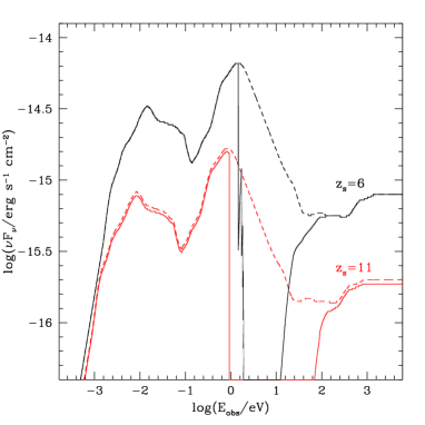
FIGURE 1.: The observed spectra of quasars with a central black hole mass of $M_{\rm bh}=10^{8}~{}{\rm M_{\odot}}$. The upper curves correspond to a source redshift of $z_{\rm s}=6$ and the lower curves to a source redshift of $z_{\rm s}=11$. In both cases we assume sudden reionization at $z_{\rm r}=10$. The dashed curves show the assumed intrinsic spectral shape, and the solid curves show the spectra after absorption by neutral intergalactic H and He.

Finally, we assume that the shape of the emitted spectrum follows the mean spectrum of known quasars (Elvis et al. 1994) up to a photon energy of 10 keV. We extrapolate the spectrum up to $\sim 50$ keV, assuming a spectral slope of $\alpha$=0 (or a photon index of -1). For reference, Figure 1 shows the adopted spectrum of quasars, assuming a black hole mass $M_{\rm bh}=10^{8}{\rm M_{\odot}}$, placed at two different redshifts, $z_{\rm s}=11$ and $z_{\rm s}=6$, and processed through the IGM, and assumed that reionization occurred at $z_{\rm r}=10$ and that at higher redshifts the IGM was homogeneous and fully neutral. At lower redshifts, $0<z<z_{\rm r}$, we included the hydrogen opacity of the Ly$\alpha$ forest given by Madau (1995), extrapolating his fitting formulae for the evolution of the number density of absorbers beyond $z=5$ when necessary. As Figure 1 shows, the minimum black hole mass detectable by the $\sim 2\times 10^{-16}~{}{\rm erg~{}s^{-1}~{}cm^{-2}}$ flux limit of CXO (see below) is $M_{\rm bh}\sim 10^{8}~{}{\rm M_{\odot}}$ at $z=10$ and $M_{\rm bh}\sim 2\times 10^{7}~{}{\rm M_{\odot}}$ at $z=5$. In our model, the corresponding halo masses are $M_{\rm halo}\sim 3\times 10^{11}~{}{\rm M_{\odot}}$, and $M_{\rm halo}\sim 6\times 10^{10}~{}{\rm M_{\odot}}$, respectively. Although such massive halos are rare, their abundance is detectable in wide-field surveys.

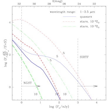
FIGURE 2.: Infrared Number Counts. The solid curves refer to quasars, while the long/short dashed curves correspond to galaxies with low/high normalization for the star formation efficiency. The curves labeled “5” or “10” show the cumulative number of objects with redshifts above $z=5$ or 10.

3. Infrared: Expected Counts with NGST

The Next Generation Space Telescope (NGST) will be able to detect the early population of mini–galaxies and mini–quasars. NGST is scheduled for launch in 2008, and is expected to reach an imaging sensitivity of $\sim 1$ nJy (S/N=10 at spectral resolution $\lambda/\Delta\lambda=3$) for extended sources after several hours of integration in the wavelength range of 1–3.5$\mu$m. Figure 2 shows the predicted number counts in the mini–galaxy and mini–quasar models described above, in a $\Lambda$CDM cosmology with ($\Omega_{0},\Omega_{\Lambda},\Omega_{\rm b},h,\sigma_{8h^{-1}},n$)=(0.35, 0.65, 0.04, 0.65, 0.87, 0.96), normalized to a $5^{\prime}\times 5^{\prime}$ field of view. This figure shows separately the number per logarithmic flux interval of all objects with redshifts $z>5$ (thin lines), and $z>10$ (thick lines). As the figure shows, NGST will be able to probe about $\sim 100$ quasars at $z>10$, and $\sim 200$ quasars at $z>5$ per field of view. The bright–end tail of the number counts approximately follows a power law, with $dN/dF_{\nu}\propto F_{\nu}^{-2.5}$. The dashed lines show the corresponding number counts of mini–galaxies, assuming that each halo undergoes a starburst that converts a fraction of 2% (long–dashed) or 20% (short–dashed) of the gas into stars. These lines indicate that NGST would detect $\sim 40-300$ mini–galaxies at $z>10$ per field of view, and $\sim 600-10^{4}$ mini–galaxies at $z>5$. Unlike quasars, galaxies could in principle be resolved if they extend over a scale comparable to the virial radius of their dark matter halos (Haiman & Loeb 1997; Barkana and Loeb 1999). The supernovae and $\gamma$-ray bursts in these galaxies might outshine their hosts and may also be directly observable (Miralda-Escudé & Rees 1997). Finally, we note that recent data in the $J$ and $H$ infrared bands from deep NICMOS observations of the HDF (Thompson et al. 1999) could already be useful to constrain mini–quasar and mini–galaxy models.

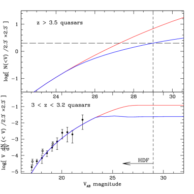
FIGURE 3.: $V$-band number counts for high–redshift quasars. The lower panel shows differential counts for $3<z<3.2$, as well as data adapted from Pei (1995). The upper panel shows cumulative number counts for $z>3.5$. The top curve shows predictions of our standard $\Lambda$CDM model with ${\rm M_{bh}\propto M_{halo}}$. The bottom curve shows the counts in a model with halo circular velocities restricted to $v_{\rm circ}\geq 75~{}{\rm km~{}s^{-1}}$. This model is consistent with the lack of detections in the HDF.

4. Optical: Constraints from the Hubble Deep Field

Although the infrared wavelengths are the best suited to detect the redshifted UV–emission from objects at $z\sim 10$, present data in the optical already yields a constraint on quasar models of the type described above. The properties of faint extended sources found in the HDF (Madau et al. 1996) agree with detailed semi–analytic models of galaxy formation (Baugh et al. 1998). On the other hand, the HDF has revealed only a handful of faint unresolved sources, but none with the colors expected for high redshift quasars (Conti et al. 1999). The simplest mini–quasar model described above predicts the existence of $\sim 10$ B–band “dropouts” in the HDF, inconsistently with the lack of detection of such dropouts up to the $\sim 50\%$ completeness limit at $V\approx 29$ in the HDF. To reconcile the models with the data, a mechanism is needed for suppressing the formation of quasars in halos with circular velocities $v_{\rm circ}\;\hbox to0.0pt{\lower 2.5pt\hbox{$\sim$}\hss}\raise 1.5pt\hbox{$<$}\;50-75~{}{\rm km~{}s^{-1}}$ (see Figure 3 for the counts). This suppression naturally arises due to the photo-ionization heating of the intergalactic gas by the UV background after reionization (Thoul & Weinberg 1996; Navarro & Steinmetz 1997). Alternative effects could help reduce the quasar number counts, such as a change in the background cosmology, a shift in the “big blue bump” component of the quasar spectrum to higher energies due to the lower black hole masses in mini–quasars, or a nonlinear black hole to halo mass relation; however, these effects are too small to account for the lack of detections in the HDF (Haiman, Madau & Loeb 1999).

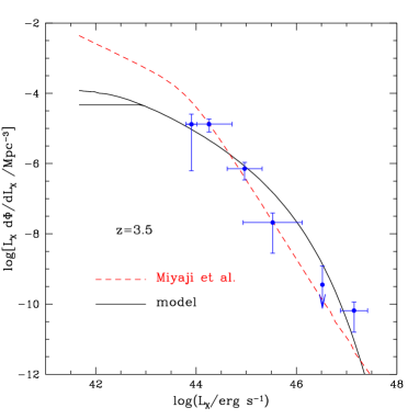
FIGURE 4.: The predicted X–ray luminosity function at $z=3.5$ in our model (solid curves). The lower curve shows the effect of a cutoff in circular velocity for the host halos of $v_{\rm circ}\geq 50~{}{\rm km~{}s^{-1}}$. The ROSAT data points are adopted from Miyaji et al. (1998a) and the dashed curve shows their fitting formula (for our background cosmology).

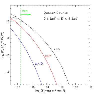
FIGURE 5.: The total number of quasars with redshift exceeding $z=5$, $z=7$, and $z=10$ are shown as a function of observed X-ray flux in the CXO detection band. The solid curves correspond to a cutoff in circular velocity for the host halos of $v_{\rm circ}\geq 50~{}{\rm km~{}s^{-1}}$, the dashed curves to a cutoff of $v_{\rm circ}\geq 100~{}{\rm km~{}s^{-1}}$. The vertical dashed line show the CXO sensitivity for a 5$\sigma$ detection of a point source in an integration time of $5\times 10^{5}$ seconds.

5. X–Rays: Predictions for CXO

Quasars can be best distinguished from star forming galaxies at high redshifts by their X-ray emission. Detections of high-$z$ quasars would therefore be highly valuable: detections, or upper limits would help in answering the important question of whether the IGM at $z\;\hbox to0.0pt{\lower 2.5pt\hbox{$\sim$}\hss}\raise 1.5pt\hbox{$<$}\;6$ was reionized by stars or quasars, by yielding constraints on the ionizing photon rate from high–$z$ quasars. The simple quasar–model described above was constructed to accurately reproduce the evolution of the optical luminosity function in the B–band (Pei 1995) at redshifts $z\;\hbox to0.0pt{\lower 2.5pt\hbox{$\sim$}\hss}\raise 1.5pt\hbox{$>$}\;2.2$ (Haiman & Loeb 1998). However, it yields good agreement with the data on the X–ray LF, as demonstrated in Haiman & Loeb (1999c), and shown here in Figure 4. We regard this model as a minimal toy model which successfully reproduces the existing data, and use a straightforward extrapolation of this model to predict the X–ray number counts. In Figure 5, we show the predicted counts in the 0.4–6keV energy band of the CCD Imaging Spectrometer (ACIS) of CXO. Note that these curves are insensitive to our extrapolation of the template spectrum beyond 10 keV. The figure is normalized to the $17^{\prime}\times 17^{\prime}$ field of view of the imaging chips. The solid curves show that of order a hundred quasars with $z>5$ are expected per field at the CXO sensitivity of $\sim 2\times 10^{-16}~{}{\rm erg~{}s^{-1}~{}cm^{-2}}$ for a 5$\sigma$ detection of a point source. Note that CXO’s arcsecond resolution will ease the separation of these point sources from background noise. The abundance of quasars at higher redshifts declines rapidly; however, a few objects per field are still detectable at $z\sim 8$. The dashed lines show the results for a minimum circular velocity of the host halos of $v_{\rm circ}\geq 100~{}{\rm km~{}s^{-1}}$, and imply that the model predictions for the CXO satellite are not sensitive to such a change in the host velocity cutoff. This is because the halos shining at the CXO detection threshold are relatively massive, $M_{\rm halo}\sim 10^{11}~{}{\rm M_{\odot}}$, and possess a circular velocity above the cutoff. In principle, the number of predicted sources would be lower if we had assumed a steeper spectral slope. For example, as figure 6 shows below, our model falls short of predicting the hard X–ray background, by about an order of magnitude at 10 keV. The difference could be explained by a change in our template spectrum to include a population of quasars with hard, but highly absorbed spectra (caused by the denser, and more gas rich hosts at high redshift). We note, however, that the agreement between the LF predicted by our model at $z\approx 3.5$ and that inferred from ROSAT observations would be upset by such a change, and require a modification of the model that would in turn tend to counter-balance the decrease in the predicted counts.

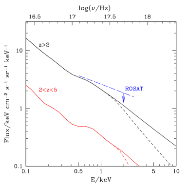
FIGURE 6.: Spectrum of the unresolved soft X–ray background in our model. We assume that the median X-ray spectrum of each source follows the mean spectrum of Elvis et al. (1994) up to 10 keV, and has a spectral slope of 0.5 (solid lines) or -0.5 (short–dashed lines) at higher photon energies. The lower curves show the spectra resulting from quasars with redshifts between $2<z<5$, and the upper curves include contributions from all redshifts $z>2$. The long–dashed line shows the unresolved fraction (assumed to be 25%) of the soft X–ray background spectrum from Miyaji et al. (1998b).

6. The X–ray Background

Existing estimates of the X–ray background (XRB) provide another useful check on our quasar model. Figure 6 shows the predicted spectrum of the XRB in our model at $z=0$ (solid lines). The unresolved background flux is shown, obtained by summing the emission of all quasars whose individual observed flux at $z=0$ is below the ROSAT PSPC detection limit for discrete sources of $2\times 10^{-15}~{}{\rm erg~{}cm^{-2}~{}s^{-1}}$ (Hasinger & Zamorani 1997). The short dashed lines show the predicted fluxes assuming a steeper spectral slope beyond 10 keV ($\alpha=-0.5$, or a photon index of -1.5). The long dashed line shows the 25% unresolved fraction of the soft XRB observed with ROSAT (Miyaji et al. 1998b; Fabian & Barcons 1992). This fraction represents the observational upper limit on the component of the soft XRB that could in principle arise from high-redshift quasars. As the figure shows, our quasar model predicts an unresolved flux just below this limit in the 0.5-3 keV range. The model also predicts that most ($\;\hbox to0.0pt{\lower 2.5pt\hbox{$\sim$}\hss}\raise 1.5pt\hbox{$>$}\;90\%$) of this yet unresolved fraction arises from quasars beyond $z=5$. The power spectrum of the unresolved background therefore might carry information on quasars at $z>5$, and be useful in constraining the models (Haiman & Hui 1999, in preparation). The correlations in the background have recently been measured by Soltan et al. (1999, see also this Proceedings).

7. Discussion

We have demonstrated that state–of–the–art X-ray observations could yield more stringent constraints on quasar models than currently available from the Hubble Deep Field (Haiman, Madau, & Loeb 1999). The X–ray data might provide the first probe of the earliest quasars, complementing subsequent infrared and microwave observations. More specifically, we have found that forthcoming X–ray observations with the CXO satellite might detect of order a hundred quasars per field of view in the redshift interval $5\;\hbox to0.0pt{\lower 2.5pt\hbox{$\sim$}\hss}\raise 1.5pt\hbox{$<$}\;z\;\hbox to0.0pt{\lower 2.5pt\hbox{$\sim$}\hss}\raise 1.5pt\hbox{$<$}\;10$. Our numerical estimates are based on the simplest toy model for quasar formation in a hierarchical CDM cosmology, that satisfies all the current observational constraints on the optical and X-ray luminosity functions of quasars. Although a more detailed analysis is needed in order to assess the modeling uncertainties in our predictions, the importance of related observational programs with CXO is evident already from the present analysis. Other future instruments, such as the HRC or the ACIS-S cameras on CXO, or the EPIC camera on XMM, which has a collective area 3–10 times larger than that of CXO, will also be useful in searching for high–redshift quasars.

The relation between the black hole and halo masses may be more complicated than linear. With the introduction of additional free parameters, a non–linear (mass and redshift dependent) relation between the black–hole and halo masses can also lead to acceptable fits (Haehnelt et al. 1998) of the observed quasar LF near $z\sim 3$. Such fits, when extrapolated to higher redshift, can result in different predictions for the abundance of high–redshift quasars. From the point of view of selecting between these alternative models, even a non–detection by CXO would be invaluable. It is hoped further that either observations of the clustering properties of $z\sim 3$ quasars in the Sloan Digital Sky Survey, or a measurement of the power spectrum of the soft X–ray background, would break model degeneracies (Haiman & Hui 1999, in preparation).

Quasars emit a broad spectrum which extends into the UV and includes strong emission lines, such as Ly$\alpha$. For quasars near the CXO detection threshold, the fluxes at $\sim 1\mu$m are expected to be relatively high, $\sim 0.5$–$0.8~{}\mu$Jy. Therefore, infrared spectroscopy of X–ray selected quasars with the Space Infrared Telescope Facility (SIRTF) or NGST can identify the redshifts of the faint X–ray point-like sources detected by the CXO satellite. Such an approach could prove to be a particularly useful approach for unraveling the reionization history of the intergalactic medium at $z\;\hbox to0.0pt{\lower 2.5pt\hbox{$\sim$}\hss}\raise 1.5pt\hbox{$>$}\;5$. At present, the best constraints on hierarchical models of the formation and evolution of quasars originate from the Hubble Deep Field. However, HST observations are only sensitive to a limiting magnitude of $V\sim 29$, and cannot probe the earliest quasars, beyond $z\sim 6$. The combination of X-ray data from the CXO satellite and infrared spectroscopy from SIRTF and NGST could potentially resolve one of the most important open questions about the thermal history of the Universe, namely whether the intergalactic medium was reionized by stars or by accreting black holes.

REFERENCES

Barkana, R., & Loeb, A. 1999, ApJ, in press, astro-ph/9906398

Baugh, C. M., Cole, S., Frenk, C. S. & Lacey, C. G. 1998, ApJ, 498, 504

Bertschinger, E. 1985, ApJS, 58, 39

Conti, A., Kennefick, J. D., Martini, P., & Osmer, P. S. 1999, AJ, 117, 645

Elvis, M., Wilkes, B. J., McDowell, J. C., Green, R. F., Bechtold, J., Willner, S. P., Oey, M. S., Polomski, E., & Cutri, R. 1994, ApJS, 95, 1

Fabian, A. C. & Barcons, X. 1992, ARA&A, 30, 429

Fan, X. et al. (SDSS collaboration) 1999, AJ, 118, 1

Haehnelt, M. G., Natarajan, P. & Rees, M. J. 1998, MNRAS, 300, 817

Haiman, Z., & Loeb, A. 1997, in Proc. of “Science with the Next Generation Space Telescope”, eds. E. Smith & A. Koratkar, p. 251

—————————– 1998, ApJ, 503, 505

—————————– 1999a, ApJ, 519, 479

—————————– 1999b, in Proc. of “After the Dark Ages: When Galaxies Were Young (the Universe at $2<z<5$)”, eds. S. Holt & E. Smith, p. 34

—————————– 1999c, ApJ, 521, 9

Haiman, Z., Madau, P., & Loeb, A. 1999, ApJ, 514

Hasinger, G., & Zamorani, G. 1997, in ”Festschrift for R. Giacconi’s 65th birthday”, World Scientific Publishing Co., H. Gursky, R. Ruffini, L. Stella eds., in press, astro-ph/9712341

Madau, P. 1995, ApJ, 441, 18

Madau, P., Ferguson, H. C., Dickinson, M. E., Giavalisco, M., Steidel, C. C., & Fruchter, A. 1996, MNRAS, 283, 1388

Magorrian, J., et al. 1998, AJ, 115, 2285

Miralda-Escudé, J. 1998, ApJ, 501, 15

Miralda-Escudé, J., & Rees, M. J. 1997, ApJ, 478, L57

Miyaji, T., Hasinger, G., & Schmidt, M. 1998a, Proceedings of “Highlights in X-ray Astronomy”, astro-ph/9809398

Miyaji, T., Ishisaki, Y., Ogasaka, Y., Ueda Y., Freyberg, M. J., Hasinger, G., & Tanaka, Y. 1998b, A&A 334, L13

Navarro, J. F., & Steinmetz, M. 1997, ApJ, 478, 13

Peacock, J. 1992, Nature, 355, 203

Pei, Y. C. 1995, ApJ, 438, 623

Press, W. H., & Schechter, P. L. 1974, ApJ, 181, 425

Rees, M. J. 1996, preprint astro-ph/9608196

Schmidt, M., Schneider, D. P., & Gunn, J. E. 1995, AJ, 110, 68

Shaver, P. A., et al. 1996, Nature, 384, 439

Songaila, A. 1997, ApJL, 490, 1

Soltan, A., et al. 1999, A&A, 349, 354

Thompson, R., et al. 1999, AJ, 117, 17

Thoul, A. A., & Weinberg, D. H. 1996, ApJ, 465, 608