Sunyaev-Zel’dovich Surveys: Analytic treatment of cluster detection

Abstract

Thanks to advances in detector technology and observing techniques, true Sunyaev–Zel’dovich (SZ) surveys will soon become a reality. This opens up a new window into the Universe, in many ways analogous to the X–ray band and inherently well–adapted to reaching high redshifts. I discuss the nature, abundance and redshift distributions of objects detectable in ground–based searches with state–of–the–art technology. An advantage of the SZ approach is that the total SZ flux density depends only on the thermal energy of the intracluster gas and not on its spatial or temperature structure, in contrast to the X–ray luminosity. Because ground–based surveys will be characterized by arcminute angular resolution, they will resolve a large fraction of the cluster population. I quantify the resulting consequences for the cluster selection function; these include less efficient cluster detection compared to idealized point sources and corresponding steeper integrated source counts. This implies, contrary to expectations based on a point source approximation, that deep surveys are better than wide ones in terms of maximizing the number of detected objects. At a given flux density sensitivity and angular resolution, searches at millimeter wavelengths (bolometers) are more efficient than centimeter searches (radio), due to the form of the SZ spectrum. Possible ground–based surveys could discover up to $\sim 100$ clusters per square degree at a wavelength of 2 mm and $\sim 10$/sq. deg. at 1 cm, modeling clusters as a simple self–similar population.

1 Introduction

Cosmologists have long appreciated the value of the Universe’s biggest objects, galaxy clusters. Besides being a collection of galaxies well suited for studies of galaxy formation, studies focussed on the global properties of clusters provide information on the nature of dark matter; the relative proportions of hot gas, dark matter and stars; and on scenarios of structure formation, including constraints on the universal density parameter, $\Omega_{\rm o}$. One example of the latter that comes to mind in anticipation of observations with the new generation of X–ray satellites, Chandra and XMM, is the use of the redshift evolution of the cluster abundance to constrain $\Omega_{\rm o}$ (Oukbir & Blanchard 1992, 1997; Bartlett 1997; Henry 1997; Bahcall & Fan 1998; Borgani et al. 1999; Eke et al. 1998; Viana & Liddle 1999a); another is the now classic cluster baryon fraction test (White et al. 1993).

While clusters have been extensively studied in the optical and X–ray bands, observations based on weak gravitation lensing and the Sunyaev–Zel’dovich (SZ) effect (Sunyaev & Zel’dovich 1972) are just coming to fruition. In the case of SZ observations, important samples consisting of several tens of clusters pre–selected in the X–ray are beginning to permit cosmologists to capitalize on the potential of combined SZ/X–ray observations (Carlstrom et al. 1996, 1999). Full maturity of the field will be heralded by the realization of purely SZ–based sky surveys. In what we might refer to as the “SZ–band”, one can then imagine performing cluster science analogous to what is now done in the X–ray, e.g., the construction of cluster counts, redshift distributions, luminosity functions, etc., all viewed via the unique characteristics of the the SZ effect. For example, several authors have emphasized the advantages of the SZ effect, over similar X–ray based efforts, to constrain $\Omega_{\rm o}$ via the cluster redshift distribution, as well as to study cluster physics out to very large redshifts (provided the clusters are out there, the very question of $\Omega_{\rm o}$ itself) (Korolyov et al. 1986; Bond & Meyers 1991; Bartlett & Silk 1994; Markevitch et al. 1994; Barbosa et al. 1996; Eke et al. 1996; Colafrancesco et al. 1997; Holder et al. 1999). Such pure SZ surveys will be performed: the Planck Surveyor will supply an almost full–sky catalog of several thousand clusters detected uniquely by their SZ signal; and advances in both detector technology and observing techniques now offer the exciting prospect of performing purely SZ–based surveys from the ground, with both large format bolometer arrays and dedicated interferometers.

I discuss in this paper some aspects of the science accessible to pure SZ surveys by examining the nature of their cluster selection. Because of the close analogy with X–ray studies, it is useful for this purpose to compare and contrast SZ–based cluster searches to those based on X–ray observations. The redshift independence of the surface brightness of a cluster (of given properties) means that SZ cluster detection is inherently more efficient than X–ray detection at finding high redshift objects. Equally important is that although the SZ effect and X–rays both “see” the hot intracluster medium (ICM), they do so in significantly different ways. In particular, the well–known fact that the SZ effect scales as the gas pressure implies that the flux density, $S_{\nu}$, is simply proportional to the total thermal energy of the gas. This makes modeling especially simple, for this quantity depends only on the total gas mass and the effectiveness of gas heating during collapse, in stark contrast to the X–ray emission that depends also on the density and temperature distribution of the gas. This simplicity is an advantage because any theoretical interpretation of survey results requires an adequately modeled relation between the observable and the theoretically relevant quantity of cluster mass.

These remarks concern essentially the physics of the ‘emission’ mechanism itself. Of equal relavence is the nature of object selection imposed by the eventual detection algorithm used to extract sources from a set of observations (a map); and this in turn depends crucially, as for any survey, on the particular combination of sensitivity and angular resolution of the observations. The objects detected by Planck will not be the same as those selected by ground–based surveys, and the final catalogs should be viewed as complementary. Planck will produce a shallow ($\sim$ tens of mJy) large–area survey, while the ground–based instruments will perform deeper surveys ($<1$ mJy) over smaller sky areas (several square degrees). Most clusters remain unresolved at the Planck resolution of $\sim 5-10$ arcmins, and this characterizes the kinds of objects accessible to this survey, e.g., the counts and the redshift distributions. The higher angular resolution of future ground–based instruments (on the order of an arcmin) will resolve many clusters and impose different selection criteria that will define the counts and redshift distributions of the final catalog.

This is a central issue of the present study were, motivated by the possibility of ground–based surveys, I examine the detection of resolved clusters. While the detection of unresolved sources is principally dependent on observational sensitivity, and the final selection is more or less one of apparent flux – $S_{\nu}\sim\theta_{\rm c}^{2}i_{\nu}$ – the detection of resolved sources is a more complicated cuisine involving individually the characteristic source size, $\theta_{\rm c}$, and surface brightness, $i_{\nu}$. The specific goal of the present work is to quantify in terms of observing parameters the abundance, masses and redshifts of clusters detectable by ground–based surveys, with the particular aims of understanding optimal object extraction and the accessible science. For example, one of the key questions facing any survey is one of observing strategy: given a fixed, total amount of observing time, should one “go deep”, with long integrations on a few fields, or instead “go wide”, covering more fields to higher sensitivity. If one is out to maximize the number of detected objects, the answer depends on the slope of the counts. One gains by going deeper if the integrated counts are steeper than $S_{\nu}^{-2}$, assuming that noise diminishes as $1/\sqrt{t}$; otherwise, a larger area yields more objects.

The cluster selection criteria of a survey may be compactly summarized by a minimum detectable mass as a function of redshift – $M_{\rm det}(z)$. Together with a suitable mass function (we shall use the formalism of Press and Schechter 1974), this quantity determines both the source counts and redshift distributions of the final source catalog. Thus, in very concrete terms, we must examine $M_{\rm det}(z)$ and understand the influence of the observationally imposed restrictions on $\theta_{\rm c}$ and $i_{\nu}$. Given a set of observations, i.e., a map, one could imagine many different algorithms to extract astrophysical sources, and $M_{\rm det}(z)$ will depend upon this choice. There is in principle an optimal method, one which preserves signal–to–noise over the entire range of source surface brightness and size. It is characterized by a decreasing surface brightness limit with object size – the greater number of object pixels permits lower surface brightness detections. This algorithm is difficult to apply in practice, and more standard approaches search instead for a minimum number of connected pixels above a preset threshold, thereby establishing a fixed cut on source surface brightness. Detection signal–to–noise is no longer constant, rather increasing with $\theta_{\rm c}$, and these methods loose large, and in–principle detectable, low surface brightness objects. All of this will be reflected in the resulting functions $M_{\rm det}(z)$.

Throughout the discussion, we will be guided by the characteristics of two potential types of ground–based instruments: large format bolometer arrays, epitomized by BOLOCAM (Glenn et al. 1998), and interferometer arrays optimized for SZ observations, as suggested by Carlstrom et al. (1999). BOLOCAM is a 151–element bolometer array under construction at Caltech for operation in three bands – 2.1 mm, 1.38 mm (the null of the thermal SZ effect) and 850 $\mu$m. At the Caltech Submillimeter Observatory, it is expected that the array will be diffraction limited to $\sim$ arcminute resolution, or better, and limited in sensitivity by atmospheric emission (rather than detector noise). With its $9$–arcmin field–of–view, one could imagine surveying a square degree to sub–mJy sensitivity in these bands. Carlstrom et al. (1999) have recently expounded the virtues of interferometric techniques using telescope arrays specifically designed for SZ observations. They have proposed the construction of such an array, operating at a wavelength of 1 cm, and estimated that it would be capable, in the course of one year of dedicated observations, of covering $\sim 10$ square degrees to a limiting sensitivity of $\sim 0.3$ mJy at arcminute resolution. In summary, then, we are interested in considering SZ observations at arcminute angular resolution and to sub–mJy sensitivity at both centimeter and millimeter wavelengths.

The paper is organized as follows: a rapid review of the SZ effect is given in the next section, followed by a discussion of the unique aspects of SZ cluster detection. Section 3 details the cluster population model employed, based on the Press–Schechter (Press & Schechter, 1974) mass function and the isothermal $\beta$–model. Since we shall focus on issues of cluster selection as imposed by survey parameters, the cluster model will be restricted to the simple example of a self–similar population. The next section (Section 4) introduces the principal figures (Figures 1,2 and 3) of the present work by consideration of unresolved cluster detection; this case will also be used as a benchmark against which to examine the effects of resolved detection. Section 5 then develops the principle themes of resolved SZ cluster detection, starting with consideration of the optimal, constant signal–to–noise method, and followed by detailed study of cluster detection based on the standard algorithm. A final discussion (Section 6) then more closely examines the number of detections to be expected from ground–based surveys and gives a non–exhaustive list of some important issues still to be treated. Section 7 concludes.

Key results will be the $M_{\rm det}(z)$ curves presented in Figure 1, quantifying the nature of SZ detected clusters, and the conclusion that resolved source counts are lower and steeper than expectations based on simple unresolved source count calculations, Figure 2. To the point, the latter implies that surveys at arcminute resolution gain objects with an observing strategy of “going deep”. The cosmological density parameter is denoted by $\Omega_{\rm o}\equiv 8\pi G\rho/3H_{\rm o}^{2}$, the vacuum density parameter by $\lambda_{\rm o}\equiv\Lambda/3H_{\rm o}^{2}$ and the Hubble constant by $H_{\rm o}\equiv h100$ km/s/Mpc; unless otherwise indicated, $h=1/2$ and $\lambda_{\rm o}=0$.

2 The Particular Value of the SZ Effect

We begin by establishing our notation in recalling the basic formulas of the SZ effect. The change in surface brightness relative to the unperturbed cosmic microwave background (CMB), caused by inverse Compton scattering in the hot ICM, is expressed as

$$i_{\nu}(\@vec{\theta})=y(\@vec{\theta})j_{\nu}(x)$$ (1)

where $x\equiv h_{p}\nu/kT_{\rm o}$ is a dimensionless frequency expressed in terms of the energy of the unperturbed CMB Planck spectrum at $T_{\rm o}=2.725\;$ K (Mather et al. cmb:temp2 (1999)). The spectral shape is embodied in the function $j_{\nu}$,

$$j_{\nu}(x) = 2\frac{(kT_{\rm o})^{3}}{(h_{p}c)^{2}}\frac{x^{4}\mbox{e}^{x}}{(\mbox{e}^{x}-1)^{2}}\left[\frac{x}{\tanh(x/2)}-4\right]$$

$$\equiv 2\frac{(kT_{\rm o})^{3}}{(h_{p}c)^{2}}f_{\nu}$$

$$= (2.28\times 10^{4}{\rm mJy/arcmin}^{2})f_{\nu}$$

while the amplitude is given by the Compton $y$–parameter

$$y\equiv\int\mbox{d}l\frac{kT}{m_{e}c^{2}}n_{e}\sigma_{T}$$ (3)

an integral of the pressure along the line–of–sight at position $\@vec{\theta}$ relative to the cluster center. Here, $T$ is the temperature of the ICM (really, the electrons), $m_{e}$ is the electron rest mass, $n_{e}$ the ICM electron density, and $\sigma_{T}$ is the Thompson cross section. Planck’s constant is written in these expressions as $h_{p}$, the speed of light in vacuum as $c$, and Boltzmann’s constant as $k$. These formulae apply in the non–relativistic limit of low electron (and photon) energies; relativistic extensions have recently been made by several authors (e.g., Rephaeli 1995; Stebbins 1997; Challinor & Lasenby 1998; Itoh et al 1998; Pointecouteau et al. 1998; Sazonov & Sunyaev 1998). The spectral shape of the distortion is unique, becoming negative at wavelengths larger than $\sim 1.4$ mm (relative to “blank” sky) and positive a shorter wavelengths. This offers a way of clearly separating the effect from other astrophysical emissions.

All of the physics is in the Compton $y$–parameter, an apparently innocuous–looking expression. In fact, it holds the key to all of the pleasing aspects of the SZ mechanism. First of all, the conspicuous absence of an explicit redshift dependence is the well–known result that the SZ surface brightness is redshift–independent, determined only by cluster properties. This should be contrasted to other emission mechanisms which all experience “cosmic dimming” [$\iota\propto(1+z)^{-4}$] due to the expansion of the Universe. This is countered in the SZ effect by the increasing energy density towards higher $z$ of the CMB, the source of photons for the effect.

Another very important aspect of the SZ mechanism resides in the fact that its amplitude is proportional to the pressure, or thermal energy, of the ICM. This appears most clearly when we consider the total flux density from a cluster, found by integrating the surface brightness over the cluster face:

$$S_{\nu}(x,M,z) = j_{\nu}(x)D_{a}^{-2}(z)\int\mbox{d}V\frac{kT(M,z)}{m_{e}c^{2}}n_{e}(M,z)\sigma_{T}$$ (4)

$$\propto M_{\rm gas}<T>$$

The integral is over the entire virial volume of the cluster. In this expression, $D_{a}(z)$ is the angular–size distance in a Friedmann–Robertson–Walker metric –

$$D_{\rm ang}(z)=2cH_{\rm o}^{-1}\left[\frac{\Omega_{\rm o}z+(\Omega_{\rm o}-2)(\sqrt{1+\Omega_{\rm o}z}-1)}{\Omega_{\rm o}^{2}(1+z)^{2}}\right]$$

$$\;=cH_{\rm o}^{-1}D(z)$$ (5)

where I introduce the dimensionless quantity $D(z)$. We see clearly that the final result is simply proportional to the total thermal energy of the ICM, $\int dVnT$. This is extremely important, because it means that the SZ flux density is insensitive (strictly speaking, completely so for the total flux density and for fixed thermal energy) to either the spatial distribution of the ICM or its temperature structure, making modeling much simpler than in the case of X–ray emission. Consider that in X–ray modeling one prefers the X–ray temperature over luminosity as a more robust indicator of cluster mass, but even the temperature has some sensitivity to the gas distribution, because it is all the same an emission weighted temperature that is actually observed. We would expect the temperature appearing in the second line of Eq. (4), which is the true mean electron energy, to demonstrate an even better correlation with virial mass than the observed X–ray temperature. Simple scaling arguments lead one to believe that this correlation should be $T\sim T_{\rm virial}\sim M^{2/3}(1+z)$, from which we deduce

$$S_{\nu}\sim f_{\rm gas}(M,z)M^{5/3}(1+z)D^{-2}(z)$$ (6)

where $f_{\rm gas}$ is the gas mass fraction contributed by the ICM to the total cluster mass.

The SZ mechanism therefore conveniently reduces all the potential complexity of the ICM to just its total thermal energy, $\propto f_{\rm gas}<T>$. This quantity may nevertheless be influenced by several factors. For example, the gas mass fraction in Eq. (6) has carefully been written as a general function of both mass and redshift. In simulations this quantity is most often constant, the majority of gas being primordial and simply falling into the cluster at formation. One could imagine other possibilities (e.g., Bartlett & Silk 1994; Colafrancesco & Vittorio 1994) that would lead to a more important dependence on either mass or redshift, although metallicity arguments seem to require that most of the gas be primordial, at least in the more massive systems (Metzler & Evrard 1994; Elbaz et al. 1995). While it appears from numerical studies that shocking during cluster formation efficiently heats the ICM to $\sim 80$%– $100$% of the virial temperature (Metzler & Evrard 1994; Bryan & Norman 1998), additional sources of heating could in principle change the temperature of the gas relative to that of the potential, i.e., $T\neq T_{\rm virial}$. Such heating may not always produce the most obvious effects – remember that it is the total thermal energy of the gas that counts, and understanding the change of this quantity with heating in a gravitational potential requires careful modeling. Although models studied so far do not lead to a strong effect (Metzler & Evrard 1994), we shall at times be discussing rather low mass systems, for which these effects are poorly understood theoretically and observationally. Finally, the exact form of the virial temperature–mass relation depends in part on the dark matter profile of the collapsing proto–cluster; once again, numerical experiments seem to indicate that this does not change too much, i.e., one finds a good T–M relation with rather small scatter (Evrard et al. 1996; Bryan & Norman 1998). Putting all of this together, a relation of the form (6) between the observable, $S_{\nu}$, and cluster mass appears quite reasonable and rather robust; and in any case, the modeling uncertainties are always easier to understand than in the case of X–rays, due to the all important insensitivity of the SZ flux density to spatial/temperature structure of the ICM.

The conclusion is that the SZ flux density should be a very good halo mass detector, in principle sensitive to all halos with significant amounts of hot gas and over a large range of redshifts. All of these remarks concern to a large extent the total SZ flux density of Eq. (4), and therefore apply primarily to situations where the clusters are unresolved. It is still true that, even when a cluster is resolved, the SZ signal is proportional to the total thermal energy of the gas, but now only of that portion contained within the column defined by the beam. After first outlining the cluster population model employed, we shall tackle in detail the additional complexities introduced by resolved cluster observations.

3 Modeling the Source Population

The central ingredient of a model for the cluster population and its evolution is the mass function, $n(M,z)$, which gives the number density of collapsed, virialized objects as a function of mass and redshift. The exact form of this function depends on the statistical properties of the primordial density fluctuations. For Inflationary–type scenarios, in which these fluctuations are Gaussian, a reasonable expression for the mass function appears to be the Press–Schechter formula (Press & Schechter 1974)

$$n(M,z)dM=\sqrt{\frac{2}{\pi}}\frac{<\rho>}{M}\nu(M,z)\left|\frac{\mbox{d}\ln\sigma(M)}{\mbox{d}\ln M}\right|\mbox{e}^{-\nu^{2}/2}\frac{dM}{M}$$ (7)

The quantity $\langle\rho\rangle$ represents the comoving cosmic mass density and $\nu(M,z)\equiv\delta_{c}(z)/\sigma(M,z)$, with $\delta_{c}$ equal to the critical linear over–density required for collapse and $\sigma(M,z)$ the amplitude of the density perturbations on a mass scale $M$ at redshift $z$. Numerical studies ascribe rather remarkable accuracy to the simple expression of Eq. (7) (Lacey & Cole 1994; Eke et al. 1996; Borgani et al. 1999), and we shall adopt it in the following. More explicitly, $\delta_{c}(z,\Omega_{\rm o},\lambda_{\rm o})$ and $\sigma(M,z)=\sigma_{\rm o}(M)\times(D_{\rm g}(z)/D_{\rm g}(0))$, with $D_{\rm g}(z,\Omega_{\rm o},\lambda_{\rm o})$ being the linear growth factor. It is essentially through $D_{\rm g}$ that the dependence on cosmology ($\Omega_{\rm o}$, $\lambda_{\rm o}$) enters the mass function, with $\Omega_{\rm o}$ being the more important of the two as the dependence on $\lambda_{\rm o}$ is relatively weak (see, e.g., Bartlett casa (1997) for a detailed discussion). This dependence on $\Omega_{\rm o}$ in the exponent means that the cluster abundance as a function of redshift is a very sensitive probe of the density parameter (e.g., Oukbir & Blanchard 1992, 1997), and is the motivation for many efforts in all wavebands to find clusters at high redshifts. As emphasized by several authors (Barbosa et al. 1996; Eke et al. 1996; Colafrancesco et al. 1997; Bartlett et al. 1998; Holder & Carlstrom 1999; Mohr et al. 1999), the SZ effect is particularly well positioned in this arena (see also below).

It is clear that the important theoretical variables are cluster mass and redshift. Although redshift is directly measurable, the mass appearing in Eq. (7) must be translated into an observational quantity suitable for the type of observations under consideration. As mentioned above, one of the pleasant features of the SZ effect is the simplicity of this relation. Using the simulations of Evrard et al. (1996) to normalize the $T-M$ relation, we can quantitatively express the total SZ flux density of a cluster (e.g., Eqs. 4 & 6) as

$$S_{\nu}=(34\,\mbox{\rm mJy}\,h^{8/3})f_{\nu}(x)f_{\rm gas}\Omega_{o}^{1/3}\left[\frac{\Delta_{\rm NL}(z)}{178}\right]^{1/3}M_{15}^{5/3}$$

$$(1+z)D^{-2}(z)$$ (8)

where the mass $M_{15}\equiv M/10^{15}\;\rm\,M_{\odot}$ refers to the cluster virial mass and $f_{\rm gas}$ is possibly a function of both mass and redshift (see also Barbosa et al. 1996, but note that the definition there of $D(z)$ differs by a factor of $2$). Evrard (1997) finds $f_{\rm gas}=0.06\;h^{-1.5}$, while Mohr et al. (1998) find marginal evidence for a decrease in lower mass systems (see also Carlstrom et al. 1999 for recent work based on SZ images); there is little information on any possible evolution with redshift at present. Other quantities appearing in this equation are the mean density contrast for virialization, $\Delta_{\rm NL}(z,\Omega_{\rm o},\lambda_{\rm o})$ ($=178$ for $\Omega_{\rm o}=1$, $\lambda_{\rm o}=0$), and the dimensionless functions $f_{\nu}$ and $D(z)$ introduced in Eqs. (2) and (2).

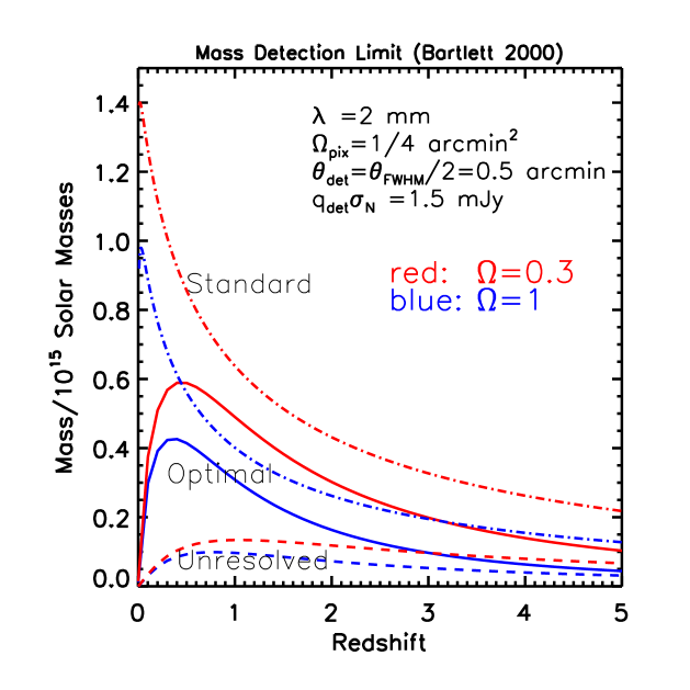
Figure 1: a)Detection mass as a function of redshift for unresolved (dashed lines), optimal resolved (solid lines) and standard resolved (dot–dashed lines) detection satisfying $q_{\rm det}\sigma_{\rm pix}=1.5$ mJy at a wavelength of $2$ mm. In the unresolved case, this simply corresponds to the limiting total flux density. For optimal resolved detection, $q_{\rm det}$ refers to $q_{\rm opt}$ in Eq. (14), while for standard resolved detection it refers to $q_{\rm st}$ of Eq. (16). The pixel size has been taken to be $\theta_{\rm fwhm}/2$, and for the standard routine a detection angle $\theta_{\rm det}=1/2\theta_{\rm fwhm}$ has been assumed, as indicated. In all cases these parameters correspond to $3\sigma$ detections (see text for more detail). The upper (red) curves in each case correspond to the open model with $\Omega=0.3$.

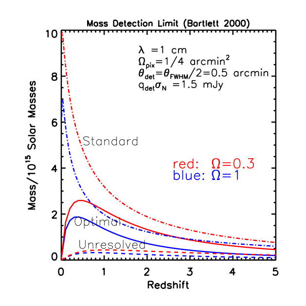
Figure 1: b)Detection mass at $1$ cm for the listed parameters. The curves are labeled as in the previous figure, but note the change in scale along the $y$–axis.

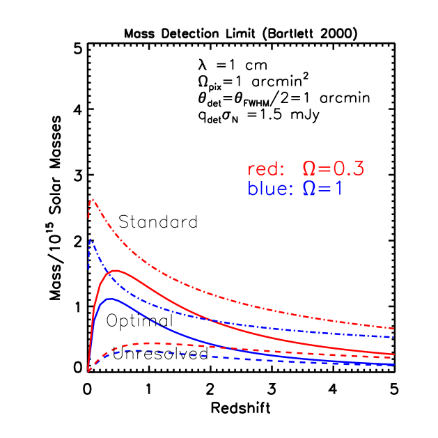
Figure 1: c)Detection mass at $1$ cm and for $\Omega_{\rm pix}=1$ arcmin² ($\theta_{\rm fwhm}=2$ arcmins). The curves are labeled as in the previous figures. Relative to Figure 1b, the lower resolution results in smaller detection masses (note again the change in ordinate scale). The unresolved detection curves are unaffected by the change in resolution.

Observations for which clusters are unresolved measure this total flux density, and therefore this is all that is needed in order to calculate the unresolved source counts, as we will do in the next section. For resolved sources, on the other hand, the detection criteria are more complicated. Contrary to the point source limit, the details of the cluster SZ profile now play an important role. I will employ a simple isothermal $\beta$–model to describe this profile:

$$i_{\nu}(\@vec{\theta})=\frac{y_{\rm o}j_{\nu}(x)}{(1+\theta^{2}/\theta_{\rm c}^{2})^{\alpha}}$$ (9)

The exponent $\alpha=0.5(3\beta-1)$, where $\beta$ is the exponent of the three–dimensional ICM density profile: $n\propto(1+r^{2}/r_{\rm c}^{2})^{-3\beta/2}$, $r_{\rm c}$ being the physical core radius. Local X–ray observations indicate that $\beta\sim 2/3$, a value I adopt throughout for the calculations. In this case, $\alpha=1/2$, a rather significant value, as will be discussed shortly. This profile will be assumed to hold out to the virial radius, $R_{\rm v}$, of the cluster.

The $\beta$–profile of Eq.(9) is empirically described by $y_{\rm o}$, a sort of central surface brightness (actually, it is $y_{\rm o}j_{\nu}$ that has units of surface brightness, but it is simpler to work with $y_{\rm o}$), and $\theta_{\rm c}$. In these terms, there is nothing specific to the SZ effect. The physics of the SZ effect appears only when we make the connection between these empirical parameters and the theoretically interesting ones, namely, mass and redshift, via relations of the kind $y_{\rm o}(M,z)$ and $\theta_{\rm c}(M,z)$. As our principle goal in this work is to understand the selection effects of resolved SZ cluster detection, the model for cluster evolution will be kept simple: a constant gas mass fraction, $f_{\rm gas}=0.06\;h^{-1.5}$ (Evrard 1997), over cluster mass and redshift, and a core radius scaling with the virial radius $R_{\rm v}$, i.e., $x_{\rm v}\equiv R_{\rm v}/r_{\rm c}=const$. Unless otherwise specified, this constant will be given a value of 10. One deduces from simple scaling arguments that

$$R_{\rm v}=(1.69h^{-2/3}{\rm\ Mpc})\;M_{15}^{1/3}(1+z)^{-1}\Omega_{o}^{-1/3}\left(\frac{178}{\Delta_{\rm NL}(z)}\right)^{1/3}$$

where the normalization is taken from the spherical collapse model. This scaling relation is about as robust as the relation for cluster temperature; in fact, the two are essentially the same, since $T\sim M/R_{\rm v}$. Some dependence of the normalization on mass and redshift could appear if the density profile around a peak forming a cluster changed significantly with these two quantities. In the following, we shall ignore this possibility, which numerical simulations seem to indicate is a small effect in any case. This then fixes the relation

$$r_{\rm c}(M,z)=R_{\rm v}(M,z)/x_{\rm v}$$ (10)

For the axially symmetric surface brightness of Eq. (9), the integral defining the total SZ flux density may be written

$$S_{\nu}(M,z) = j_{\nu}2\pi\int d\theta\theta\;y(\theta)$$

$$= 2\pi j_{\nu}y_{\rm o}(M,z)\theta_{\rm c}^{2}(M,z)\left(\sqrt{1+x_{\rm v}^{2}}-1\right)$$

Using Eq. (3) for $S_{\nu}(M,z)$ in this expression, we deduce

$$y_{\rm o}(M,z) = (6.40\times 10^{-5}h^{2})f_{\rm gas}\Omega_{\rm o}\left(\frac{\Delta_{\rm NL}(z)}{178}\right)$$ (11)

$$M_{15}(1+z)^{3}\left(\frac{x_{\rm v}^{2}}{\sqrt{1+x_{\rm v}^{2}}-1}\right)$$

Together with the $\beta$–profile (Eq. 9), Eqs. (10) and (11) define our cluster evolution model. As mentioned, it is self–similar, and we see the expected scaling $r_{\rm c}\sim M^{1/3}/(1+z)^{-1}$ and $y_{\rm o}\sim M(1+z)^{3}$. This is most probably an oversimplified description of the actual cluster population, but it nevertheless provides a ‘standard’ with which we may understand the nature of the selection effects imposed by resolved cluster detection, and a benchmark for comparing more detailed models. It is important in the following that one does not forget the model dependence of our results, which can be retraced to this point of the discussion.

4 Unresolved Detections

This section is dedicated to the simple case of unresolved SZ detection, which will be used as a reference in the following discussion of resolved detection. It also offers an introduction to the main figures, Figures 1, 2 and 3, summarizing the essential results of the present work. They are constructed for two representative cosmologies: a critical model $\Omega_{\rm o}=1$, and an open model ($\lambda_{\rm o}=0$) with $\Omega_{\rm o}=0.3$. For the counts and redshift distributions of Figures 2 and 3, I have used a CDM–like power spectrum with “shape parameter” fixed at $\Gamma=0.25$; both models are normalized to the present day abundance of X–ray clusters – $\sigma_{8}=0.6$ and $\sigma_{8}=1.0$ for the critical and open models, respectively (e.g., Blanchard et al. 1999; Borgani et al. 1999; Viana & Liddle 1999b).

Observations for which most clusters are unresolved measure the total SZ flux density. One can then simply invert Eq. (3) to find the corresponding limiting detection mass as a function of redshift, $M_{\rm det}^{\rm ur}(z,S_{\nu})$:

$$M_{\rm det}^{\rm ur}(z,S_{\nu}) = (0.12\times 10^{15}h^{-8/5}\rm\,M_{\odot})\left(\frac{S_{\nu}}{{\rm mJy}}\right)^{3/5}$$ (12)

$$(f_{\nu}f_{\rm gas})^{-3/5}\Omega_{\rm o}^{-1/5}\left(\frac{178}{\Delta_{\rm NL}}\right)^{1/5}$$

$$D^{6/5}(z)(1+z)^{-3/5}$$

Integrating the mass function over redshift and over masses greater than this limit directly yields the source counts:

$$\frac{dN}{d\Omega}(>S_{\nu})=\int_{0}^{\infty}dz\frac{dV}{dzd\Omega}\int_{M_{\rm det}(z,S_{\nu})}^{\infty}dM\;\frac{dn}{dM}(M,z)$$ (13)

The corresponding redshift distribution is simply obtained as the integrand of the $z$–integral.

Figure 1 compares the various detection masses as a function of redshift for observations at $2$ mm, e.g., a bolometer array, and at $1$ cm, representative of an interferometer; in each case the upper (red) curve corresponds to the open model. For the moment, concentrate only on the the dashed lines, which give the result for unresolved detection, Eq. (12), at a flux density of $S_{\nu}=1.5$ mJy. These curves remain unchanged from Figure 1b to 1c, both at $1$ cm but differing in angular resolution, because resolution is irrelevant for point sources (ignoring source confusion issues). Observe that in all cases the detection mass decreases with redshift beyond $z\sim 1$. This remarkable behavior is directly attributable to the fact that the SZ surface brightness is independent of distance. As already emphasized, the distance appearing in Eq. (12) is the angular distance and not the luminosity distance, a factor of $(1+z)^{2}$ larger. At high $z$ the redshift dependence therefore scales as $\sim z^{-9/5}$, one power coming from the assumed redshift scaling of the virial temperature and the rest from the decrease in angular distance (focusing) as $\sim 1/z$. A self–similar cluster model, implicitly assumed in this context by the constancy of $f_{\rm gas}$, thus predicts that SZ observations are more sensitive to objects at large, rather than intermediate, redshifts. This overall behavior would not change even if we broke the self–similarity with a declining gas mass fraction with mass; such a dependence could only modify the rate of decrease with $z$. On the other hand, an explicit decrease in $f_{\rm gas}$ with redshift stronger than $(1+z)^{-3}$ would cause $M_{\rm det}^{\rm ur}$ to actually increase with redshift. It is perhaps not so surprising that at close range, small $z$, the detection mass also drops; this is simply due to the increasing angular size of the object creating an increase in total flux density (the source is assumed to always remain unresolved in this discussion).

From the difference between Figures 1a and 1b,c, we see that, at a given sensitivity, the $2$ mm observations probe farther down in mass. This is nothing more than the spectral shape of the SZ effect, described by the function $j_{\nu}$: the biggest decrement occurs precisely near $2$ mm (the maximum emission of the effect is around $750\mu$m). The resolved detection mass limits, to be shortly discussed, depend also on the angular resolution.

Source counts for the two cosmological scenarios are given in Figure 2. These have been calculated using Eq. (13) and the appropriate detection mass. In order to shed some light on the importance of low mass objects to these results, the counts are presented in pairs, one curve for a low mass cut–off of $10^{13}\;\rm\,M_{\odot}$ and one for a cut–off of $10^{14}\;\rm\,M_{\odot}$. Note that the $x$–axis denotes the pixel noise, $\sigma_{\rm pix}$, and not a limiting source flux density; in the present situation of unresolved detections, this just means that the corresponding limiting flux density is $q_{\rm det}\times\sigma_{\rm pix}$.

The first thing to remark from Figure 2 is the large difference between the two cosmological models. The presence of clusters at high redshift in a low–density model shows up in the integrated counts, as confirmed by the corresponding redshift distributions shown in Figure 3, where the huge difference in cluster abundance at large redshift is evident. It is for this reason that the redshift distribution of SZ sources is a potentially powerful tool for constraining $\Omega_{\rm o}$ (Barbosa et al. 1996, Bartlett et al. 1998). This is of foremost importance and represents one of the primary motivating factors behind this type of survey.

This situation of unresolved sources applies in practice to missions such as the Planck Surveyor, as discussed, for example, by Barbosa et al. (1996) and Aghanim et al. (1997). The higher angular resolution of possible ground–based surveys calls for examination of resolved source detection.

5 Resolved Detections

In this, the principle section of this paper, we treat in detail the issue of resolved SZ cluster detection. The context will be one of arcminute resolution (pixel size) and sub–mJy sensitivity, as targeted by the up–coming ground–based instruments. It is worth being very explicit about the nature of the observations: the simplest case to imagine corresponds to that of an image produced by a bolometer array, such as BOLOCAM. In this case each point on the image, a ‘pixel’, represents a sample point of the sky brightness, as transformed by the optics of the observing system. The optical response may be divided into that of the telescope–plus–atmosphere (defining the projection of the sky onto the focal plane) and the optics proper to the detector (which act on the focal–plane image). There is a difference between bolometer arrays and the familiar example of a CCD camera working in the visible. For the latter, atmospheric seeing and telescope optics project the sky onto the focal plane by convolving with a Gaussian, and the camera itself then convolves this focal–plane image with a square top–hat, one centered on each pixel. The difference with a bolometer array lies in the fact that the CCD camera defines sharp, well–defined pixel boundaries, while a bolometer array, with its set of cones, convolves the focal–plane image with something closer to a Gaussian. This means that, unlike CCDs, the pixels of a bolometer array ‘overlap’ in the focal plane. This has little consequence for the ensuing discussion, but it is all the same worth keeping in mind.

This picture is not completely accurate when it comes to interferometers. Such instruments actually directly sample the Fourier transform of the sky. The result may often be modeled by a real sky image convolved with an effective, synthesized beam, but this beam lacks sensitivity on large scales, i.e., large spatial wavelengths on the sky (short baselines). Thus, the effective beam cannot not be precisely a Gaussian, and it is especially important to correctly model the loss of response on large scales for extended objects such as clusters. For the ensuing discussion, I adopt the bolometer picture, applying it at times rather indiscriminately to characterize ground–based observations; a future work will consider the details specific to interferometric observations (see also the recent work of Holder et al. 1999).

For a bolometer array, the response of the entire optical chain (atmosphere-telescope-detector) is often adequately modeled as a bi–dimensional Gaussian (if one is lucky, a symmetric one!), and for proper sampling, respecting Shannon, the sample period must be 2 – 3 times smaller than the beam FWHM. We will characterize a survey by the pixel size and sensitivity per pixel of its images – $\Omega_{\rm pix}$, a solid angle, and $\sigma_{\rm pix}$, a flux density. Note that because the pixels ‘overlap’ in the focal plane, what precisely is meant by $\Omega_{\rm pix}$ is the square of the separation between sample points, $\theta_{\rm pix}$; the concept is a bit more ambiguous than in the case of a CCD camera. Thus, proper sampling means that the pixel scale $\Omega_{\rm pix}\equiv\theta_{\rm pix}^{2}\leq\theta_{\rm fwhm}^{2}/4$. It is also worth explicitly remarking that, in the following, I assume that the noise is uncorrelated (from pixel to pixel) and uniform over the image.

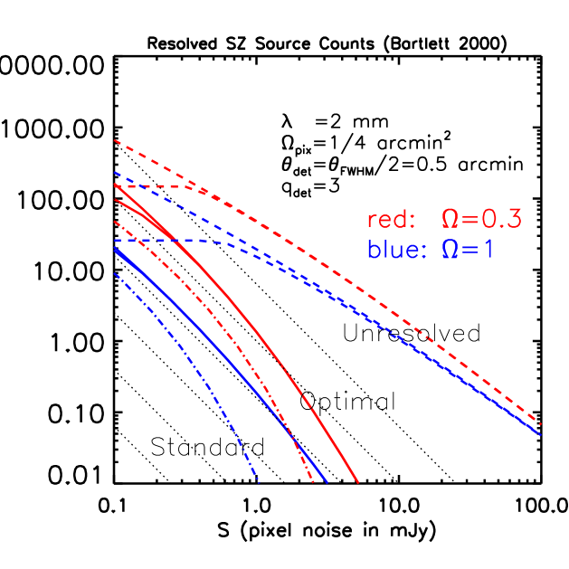
Figure 2: a) Cluster integral source counts at $2$ mm as a function of map pixel noise for the two cosmological models introduced in the text. The angular resolution and sampling correspond to the situation of Figure 1a. Unresolved, optimal resolved and standard resolved counts are shown, respectively, as the dashed, solid and dot–dashed lines; the upper (red) curve in each case corresponds to the open model with $\Omega=0.3$. For unresolved detections, the limiting source flux density is simply $q_{\rm det}\times$(pixel noise). The light dotted lines in the background indicate the critical slope of $-2$. The fact that the resolved counts are steeper than this value implies that, down to low noise levels, deep integrations yield more objects than wide and shallow ones.

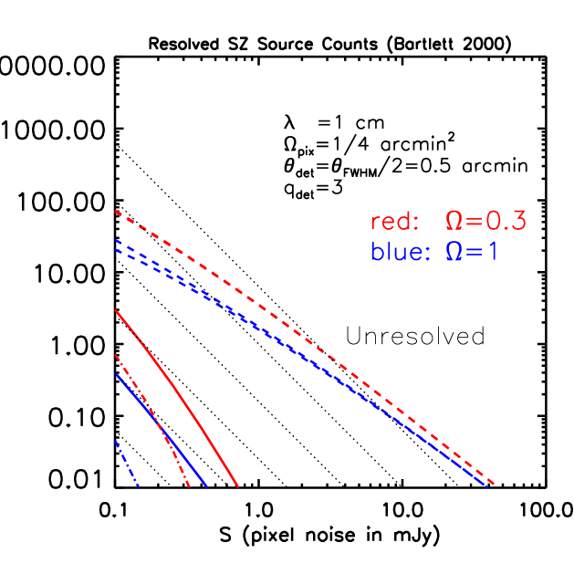
Figure 2: b) Same as the previous figure for an observation wavelength of $1$ cm; curve types have the same meaning as before (the labels ‘Optimal’ and ‘Standard’ have been removed for clarity). The resolution and sampling correspond to the situation of Figure 1b.

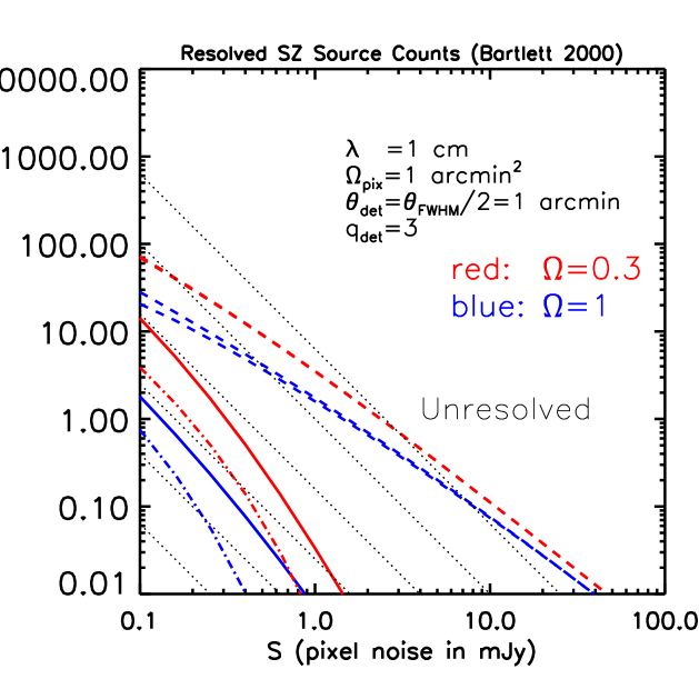
Figure 2: c) Same as Figure 2b ($\lambda=1$ cm) but now for $\Omega_{\rm pix}=1$ arcmin², i.e., the situation of Figure 1c. The smaller detection masses at this lower resolution result in higher counts when compared to Figure 2b. Note that the unresolved counts are the same here as in Figure 2b.

Given, then, a map of the SZ sky, we would like to understand how to extract clusters and the nature of the selection imposed by our technique. In addition to the observational parameters $\Omega_{\rm pix}$ and $\sigma_{\rm pix}$, this will depend on the form of the extended emission of the sources, a complication avoided in the case of unresolved cluster detection; this represents an important difference between the two situations. Employing the $\beta$–model introduced previously, Eq. (9), we see that a cluster SZ profile may be described by a characteristic central surface brightness, $y_{\rm o}$, and an angular size, $\theta_{\rm c}$ (the core radius). When couched in terms of the purely empirical parameters of $\Omega_{\rm pix}$, $\sigma_{\rm pix}$, $y_{\rm o}$ and $\theta_{\rm c}$, we have before us a rather classic and well–known problem of Astronomy. The only difference with galaxies in the optical is the form of the source profile. All physics specific to the SZ effect itself appears only in the relation of the empirical source descriptors – $(y_{\rm o},\theta_{\rm c})$ – to the theoretically meaningful ones of cluster mass, $M$, and redshift, $z$.

The procedure in the following is then always the same: quantify the detection algorithm in terms of $\Omega_{\rm pix}$ and $\sigma_{\rm pix}$, and then translate this, via the isothermal $\beta$–model, into a $M_{\rm det}(z;\Omega_{\rm pix},\sigma_{\rm pix})$. I employ a notation where the imminently interesting independent variables of a function appear before the “;”, and parameterizing ones afterward. Thus, as written, the detection mass is primarily a function of redshift, parameterized by the survey properties $\Omega_{\rm pix}$ and $\sigma_{\rm pix}$. This function teaches us about the kinds of objects we detect, and leads directly to the survey counts and the redshift distribution of our clusters, via Eq. (13). These latter quantities are the key indicators of the science content of the survey.

This procedure will be applied to two source extraction methods in the following, and the results compared to those for an unresolved SZ survey. We will refer to the first as “optimal detection”, because it extracts sources in such a way as to preserve the signal–to–noise across the entire range of detectable surface brightness and source size. This is achieved by lowering the surface brightness limit for large sources, possible due to the greater number of covered pixels. The second method, routinely used by such packages as SExtractor (Bertin & Arnouts 1996), searches for a minimum number of connected pixels above a preset threshold. The important difference with the first technique is the imposition of a fixed surface brightness limit, independent of source size. The signal–to–noise of the detections is no longer constant, but increases with source size. This technique may be considered sub–optimal in the sense that it loses in–principle detectable low surface brightness sources, a fact well appreciated in the case of optical galaxy surveys.

5.1 Optimal case

Optimal detection selects all sources with a flux density

$$S_{\nu}\geq q_{\rm opt}N^{1/2}\sigma_{\rm pix}$$

(assuming spatially uncorrelated and uniform noise) where $N$ is the number of pixels covered by the cluster and $q_{\rm opt}$ represents a threshold, say $q_{\rm opt}\sim 3-5$; in fact, $q_{\rm opt}=S/N$, the signal–to–noise of the detection. Notice also that, as advertised, the limiting surface brightness decreases with object size: $<i_{\nu}>\sim S_{\nu}/N\sim q_{\rm opt}\sigma_{\rm pix}/\sqrt{N}$. One extracts in this way all objects detectable at a given $S/N$, and for this reason we may refer to the method as optimal. The number of object pixels is simply found as $N=\pi\theta_{\rm vir}^{2}/\Omega_{\rm pix}$, where $\theta_{\rm vir}=R_{\rm v}/D_{\rm ang}$ is angular virial radius. This permits us to express the detection mass as

$$M_{\rm det}^{\rm opt}(z,S_{\nu}) = (0.19\times 10^{15}h^{-2}\rm\,M_{\odot})\left(\frac{q_{\rm opt}\sigma_{\rm pix}}{\rm mJy}\right)^{3/4}$$ (14)

$$\left(\frac{{\rm arcmin}^{2}}{\Omega_{\rm pix}}\right)^{3/8}(f_{\nu}f_{\rm gas})^{-3/4}\Omega_{\rm o}^{-1/2}$$

$$\left(\frac{178}{\Delta(z)}\right)^{1/2}D^{3/4}(z)(1+z)^{-3/2}$$

As written, this criteria uses an aperture corresponding to the full angular size of the object – $S_{\nu}$ is understood to be the total SZ flux density in Eq. (3). For resolved sources, one would like to chose an aperture which optimizes the signal–to–noise ratio of the detection. Interestingly, a 3D gas profile close to $r^{-2}$, corresponding to a SZ surface brightness $y\propto\theta^{-1}$, results in a constant signal–to–noise with aperture radius. A $\beta$–model with $n\propto(1+r^{2}/r_{\rm c}^{2})^{-3\beta/2}$ and $\beta\sim 2/3$ exhibits this behavior at large radii, for example: $y(\theta)\sim(1+\theta^{2}/\theta_{c}^{2})^{-1/2}$. In this case, the signal–to–noise of a SZ detection increases from the center of the cluster image out to the core radius, $r_{\rm c}$, beyond which it turns over to a constant out to the virial radius. The situation is different for X–ray images, where the surface brightness falls off more rapidly, diving under the background at large radii. From this we conclude that the simple criteria given above provides in fact an optimum SZ detection (at least as long as $\beta$ remains close to 2/3, as appears to be the case locally).

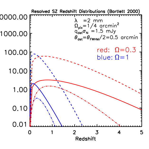
Figure 3: a) Redshift distribution of the integrated counts for a flux density of $q_{\rm det}\sigma_{\rm pix}=1.5$ mJy at $2$ mm. The parameters are the same as those in Figure 2a, and the line types have the same meaning. The upper (red) curve in each case corresponds to the open model with $\Omega_{\rm o}=0.3$. Note the large difference between the two cosmological models apparent in all cases.

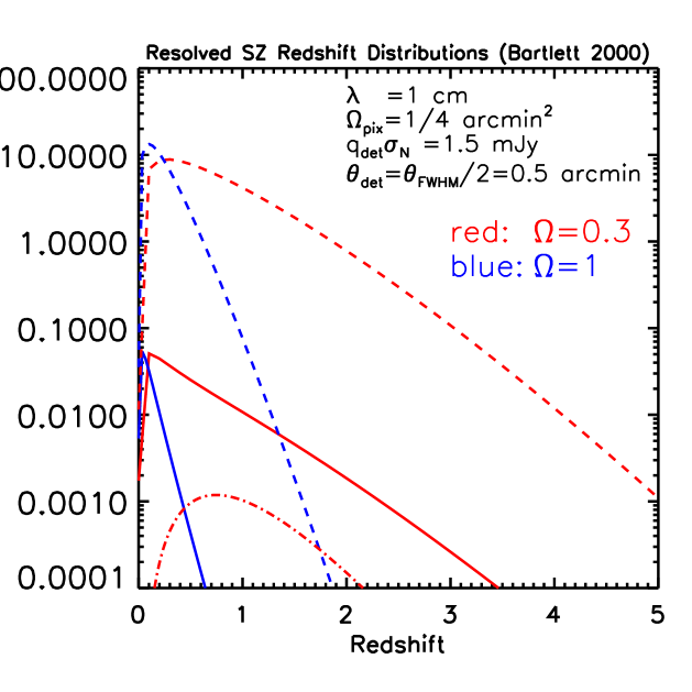
Figure 3: b) Redshift distribution of the integrated counts for a flux density of $q_{\rm det}\sigma_{\rm pix}=1.5$ mJy at $1$ cm, and for the same parameters as in Figure 2b.

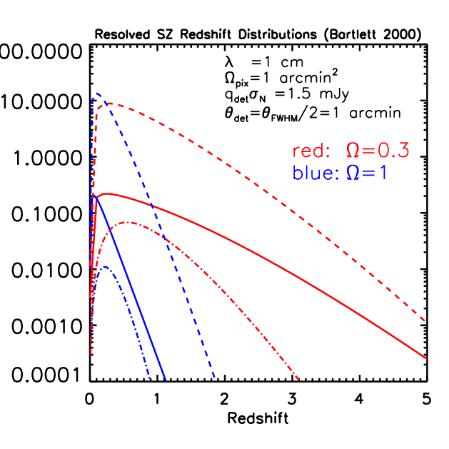
Figure 3: c) Redshift distribution of the integrated counts for a flux density of $q_{\rm det}\sigma_{\rm pix}=1.5$ mJy at $1$ cm, and for the same parameters as in Figure 2c; in particular, for $\theta_{\rm fwhm}=2$ arcmins.

The detection mass Eq. (14) is displayed in Figure 1 as the solid lines. Compared to the hypothetical point source results, observations resolving clusters are less efficient at detecting clusters, especially at intermediate redshifts. This is easy to understand as the effect of distributing a given flux density over $N$ pixels, each adding a noise with variance of $\sigma_{\rm pix}$, resulting in a total noise level over the object image of $\sqrt{N}\sigma_{\rm pix}$. A point source, in contrast, is only subject to the noise of one pixel, $\sigma_{\rm pix}$. Hence, high resolution at fixed sensitivity “resolves out” a certain fraction of objects. The consequences for the source counts are clear and will be discussed shortly. These curves retain the same asymptotic behavior as before, namely a greater sensitivity to low masses at high redshift. Despite the fact that the object covers a larger number of noisy pixels as $z$ decreases, the optimal method is able to take proper advantage of the greater total flux density to detect low mass objects locally, just as in the case of unresolved point sources. We shall see that this does not follow for the standard detection routine (the dot–dashed lines), due to its additional surface brightness constraint (discussed below). By comparing Figures 1b and 1c, which differ only in their angular resolution, we note that for a given sensitivity, lower resolution observations are the more effective. This is traceable to the fact that the flux density of a source is dispersed over fewer (noisy) pixels than would be the case at a higher angular resolution. This indicates that low resolution observations at a given wavelength and sensitivity are to be prefered, at least for detection purposes. There is, however, a limit set by eventual source confusion.

We have just seen from Figure 1 that low surface brightness clusters are “resolved out” at high resolution. This leads to overall lower counts that are also much steeper than the equivalent for unresolved point sources. Generally speaking, the unresolved counts do not deviate too much from a Euclidean law, $\propto S_{\nu}^{-3/2}$; on the other hand, the resolved counts can be much steeper. The examples shown in Figure 2 are in fact steeper than $S_{\nu}^{-2}$, indicated by the dotted lines, down to essentially the faintest flux levels attainable in immediately foreseeable observations. This is critical for optimizing an observing strategy with a fixed amount telescope time, $T$. Consider the common situation in which the final map noise decreases with integration time as $1/\sqrt{t}$; then, the solid angle covered in time $T$, with individual field integrations of duration $t$, scales with sensitivity as $\sim T/t\sim\sigma_{\rm pix}^{2}$. Hence, if the integrated source counts are steeper than $\sigma_{\rm pix}^{-2}$, one gains objects by “going deep”, integrating longer on each individual field, rather than “going wide”, with shorter integrations covering a larger total solid angle. The important conclusion to draw from Figure 2 is then that the way to optimize the number of detected objects in a survey with arcminute resolution is by “going deep”, down to the point were the counts begin to flatten out. In our examples, this does not occur until the very lowest flux levels deemed at present reasonable. It should be emphasized that this conclusion rests on the results calculated here in the context of a self–similar cluster population. It is all the same suggestive and important in the fact that it is contrary to the conclusion one would draw based on unresolved source count calculations. The opposite holds for surveys with low angular resolution where the majority of sources remain unresolved, such as the Planck Surveyor observations.

Finally, as to be expected from the “loss” of objects at intermediate redshifts, the redshift distribution for optimally selected objects lies under the corresponding point source examples, and is somewhat flatter. All the same, the two cosmological models are easily distinguished with an enormous “leverage” at high $z$.

5.2 Standard algorithms

Standard detection routines typically identify sources as a minimum number of contiguous pixels all above a preset threshold, usually $q_{\rm st}$ times the pixel noise $\sigma_{\rm pix}$. This is not the same criteria as above, in the optimal case, because we have now established a fixed surface brightness threshold – $q_{\rm st}\sigma_{\rm pix}/\Omega_{\rm pix}$ – independent of object size (or luminosity). Previously, we allowed ourselves to lower this threshold for larger sources, in order to pick–up low surface brightness objects while maintaining a constant signal–to–noise; for this reason, it was an optimum detection algorithm. Here, the surface brightness is instead a fixed, while the signal–to–noise increases with object size as $S/N=q_{\rm st}\sqrt{N}$. A further difference is that the surface brightness cut imposes a minimum detectable mass at $z=0$. We obviously expect this method to detect fewer objects than the optimal approach.

Consider application of the standard algorithm to a SZ profile, empirically described in the $\beta$–model by $y_{\rm o}$ and $\theta_{\rm c}$. Although our final goal is to understand the selection on mass and redshift imposed by the detection criteria, it is quite useful, firstly, to gain insight into the workings of detection in terms of $y_{\rm o}$ and $\theta_{\rm c}$. As mentioned, what is actually recorded at each sample point (pixel), say by a bolometer camera, is the sky signal integrated over the beam $B$, which we will take to be axially symmetric. Thus, for a pixel at position $\hat{n}$ (a unit vector on the sphere):

$$S_{\nu}^{\rm obs}(\hat{n})=\int d\Omega^{\prime}i_{\nu}(\hat{n}^{\prime})B(\hat{n}\cdot\hat{n}^{\prime})$$

For our calculations, we shall furthermore adopt a Gaussian beam, so that a cluster appears as a $\beta$–profile smeared by a Gaussian of dispersion $\sigma_{\rm b}=\theta_{\rm fwhm}/\sqrt{8\ln 2}$,

$$B=e^{-\theta^{2}/2\sigma_{\rm b}^{2}}$$

where $\theta$ is the angle from the beam axis and $\theta_{\rm fwhm}$ is the beam full–width at half–maximum. Notice that we take the image to be in flux density units. By placing the coordinate origin at the cluster center, so that now $\hat{n}$ is simply marked by the angular distance $\@vec{\theta}$ from the origin (small angle approximation), the beam–smeared profile of a cluster may be written as

$$S_{\nu}^{\rm obs}(\theta)=y_{\rm o}\theta_{\rm c}^{2}j_{\nu}{{\cal G}}[\theta/\theta_{\rm c};\sigma_{\rm b}/\theta_{\rm c}]$$

explicitly separating out a dimensionless function

$${{\cal G}}(r;p) \equiv \int_{0}^{\infty}dx\;xe^{-\frac{1}{2}\left(\frac{x}{p}\right)^{2}}$$

$$\int_{0}^{2\pi}d\phi\;\frac{\Theta[x_{\rm v}^{2}-r^{2}-x^{2}-2xr\cos\phi]}{\left(1+r^{2}+x^{2}+2xr\cos\phi\right)^{\alpha}}$$

parameterized only by the ratio $p=\sigma_{\rm b}/\theta_{\rm c}$. The Heavyside function, $\Theta$, cuts off the integral beyond the virial radius.

It is this smeared profile of a cluster that is subject to the detection criteria that a minimum number of connected pixels, $N_{\rm min}$, must lie above the threshold $q_{\rm st}\sigma_{\rm pix}$. This amounts to demanding that the object image above a flux density of $q_{\rm st}\sigma_{\rm pix}$ cover a minimum solid angle of $N_{\rm min}\Omega_{\rm pix}$. Let $\theta_{\rm det}$ be the angular size of a cluster above the detection threshold, which may be calculated as the root of the following equation:

$$S_{\nu}^{\rm obs}(\theta_{\rm det})=q_{\rm st}\sigma_{\rm pix}$$ (15)

We will say that a cluster is detected if $\theta_{\rm det}$ is large enough to cover $N_{\rm min}$ pixels. In the present analytic treatment, we will simply impose a lower limit to $\theta_{\rm det}$ and ignore any complications arising from the discreteness of the image. Using the function ${\cal G}$, Eq. (15) may be written in compact form as

$${\cal G}[\theta_{\rm det}/\theta_{\rm c};\sigma_{\rm b}/\theta_{\rm c}]=\frac{q_{\rm st}\sigma_{\rm pix}}{y_{\rm o}\theta_{\rm c}^{2}j_{\nu}}\equiv\frac{\hat{y}}{y_{\rm o}}\left(\frac{\sigma_{\rm b}}{\theta_{\rm c}}\right)^{2}$$ (16)

introducing the parameter $\hat{y}\equiv(q_{\rm st}\sigma_{\rm pix})/(\sigma_{\rm b}^{2}j_{\nu})$ characterizing the experimental set–up. It is clear that the solution will be given as $\theta_{\rm det}/\theta_{\rm c}$, that it will be a function of $\sigma_{\rm b}/\theta_{\rm c}$ and $y_{\rm o}$, and that it will be parameterized by $\hat{y}$, i.e.,

$$[\theta_{\rm det}/\theta_{\rm c}](\sigma_{\rm b}/\theta_{\rm c},y_{\rm o};\hat{y})$$

To understand the role of $\hat{y}$, study the result in the limit as $\theta_{\rm c}\rightarrow\infty$; this will be particularly important below, when we consider the non–zero detection mass at zero redshift imposed by the surface brightness cut. In this large–object limit, ${\cal G}(r;p)\rightarrow{\cal G}(r\rightarrow 0;p\rightarrow 0)\rightarrow 2\pi p^{2}$. We thus find that in order to be detected an object must have a central surface brightness

$$y_{\rm o}>\frac{\hat{y}}{2\pi}$$ (17)

In other words, $\hat{y}$ indeed embodies the surface brightness cut. This will be used shortly.

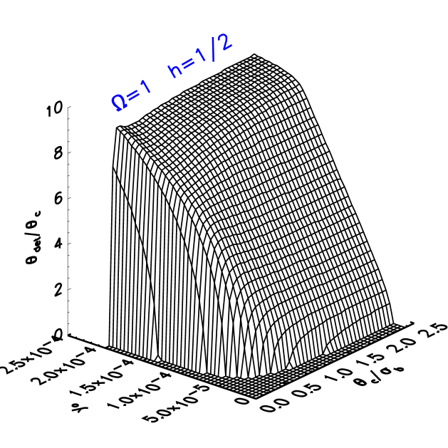
Figure 4: a) The behavior of $\theta_{\rm det}/\theta_{\rm c}$ as a function of $\theta_{\rm c}/\sigma_{\rm b}$ and $y_{\rm o}$ in a critical–density universe ($\Omega=1$, $h=1/2$) and for $|\hat{y}|=9.48\times 10^{-5}$, e.g., $\lambda=2$ mm, $\theta_{\rm fwhm}=1$ arcmin and $q_{\rm det}\sigma_{\rm pix}=1.5$ mJy.

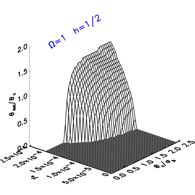
Figure 4: b) Same as Fig. 4a, but for $|\hat{y}|=6.84\times 10^{-4}$, e.g., $\lambda=1$ cm, $\theta_{\rm fwhm}=1$ arcmin and $q_{\rm det}\sigma_{\rm pix}=1.5$ mJy (or $\lambda=2$ mm, $\theta_{\rm fwhm}=1$ arcmin and $q_{\rm det}\sigma_{\rm pix}=11$ mJy, or $\lambda=2$ mm, $\theta_{\rm fwhm}=2.69$ arcmins and $q_{\rm det}\sigma_{\rm pix}=1.5$ mJy).

Figure 4 shows the solution over the $(\theta_{\rm c}/\sigma_{\rm b},y_{\rm o})$–plane for two reasonable values of $|\hat{y}|$. To understand this figure, separate the plane into a region occupied by resolved sources – $\theta_{\rm c}/\sigma_{\rm b}>>1$ – and the region of point sources, $\theta_{\rm c}/\sigma_{\rm b}<<1$:

• Resolved sources: It is clear that by increasing $y_{\rm o}$ at fixed $\theta_{\rm c}/\sigma_{\rm b}(>>1)$, we see an ever increasing portion of the ICM. The cluster ‘lights-up’ until we see all of it, out to the virial radius (beyond which we assume that the gas has not been heated), and the solution flattens out at this point to the adopted value $x_{\rm v}=R_{\rm v}/r_{\rm c}=10$; beyond this, there is no more cluster to be seen. Of course, in the other direction, the object is eventually lost as we decrease $y_{\rm o}$ to the point where even the central parts of the cluster do not rise above the detection threshold.

• Point–source limit ($\theta_{\rm c}/\sigma_{\rm b}\rightarrow 0$): In this extreme, the source profile becomes that of the beam, normalized to the total source flux density. This latter quantity scales as $y_{\rm o}j_{\nu}\theta_{\rm c}^{2}$, so that as $\theta_{\rm c}/\sigma_{\rm b}$ continues to decrease at fixed $\hat{y}$ (i.e., holding $\sigma_{\rm b}$ constant), the imprint of the object gradually sinks below the detection threshold and $\theta_{\rm det}\rightarrow 0$; this explains the cut-off at low $\theta_{\rm c}/\sigma_{\rm b}$ for a given central surface brightness.

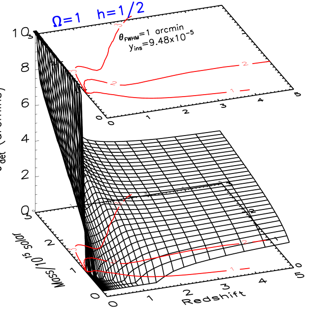
Figure 5: a) Source detection radius (arcmins) as a function of cluster mass $M$ (units of $10^{15}$ solar masses) and redshift, for $\theta_{\rm fwhm}=1$ arcmin and $\hat{y}=9.48\times 10^{-5}$, e.g., $\lambda=2$ mm and $q_{\rm st}\sigma_{\rm pix}=1.5$ mJy. Notice the non–zero detection mass at $z=0$.

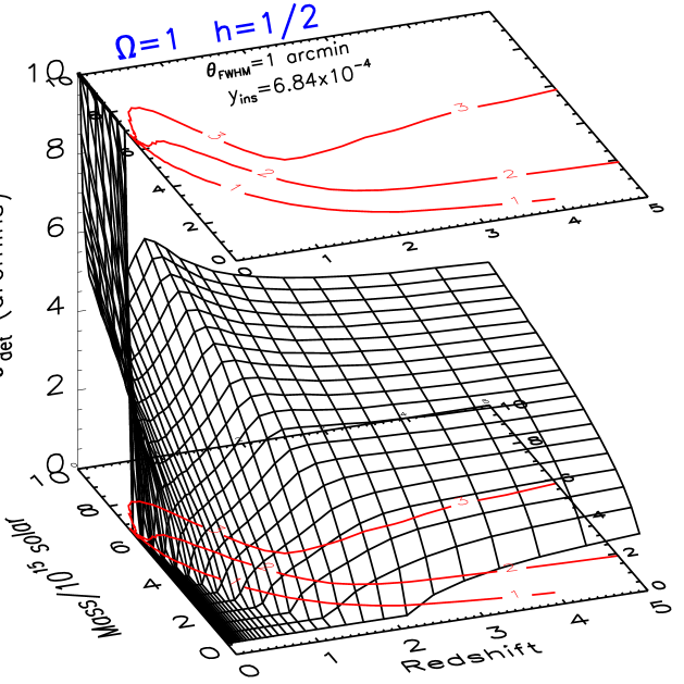
Figure 5: b) Source detection radius for $\theta_{\rm fwhm}=1$ arcmin and $\hat{y}=6.84\times 10^{-4}$, e.g., $\lambda=1$ cm and $q_{\rm st}\sigma_{\rm pix}=1.5$ mJy. Note the change of scale for the $M$–axis relative to the previous figure.

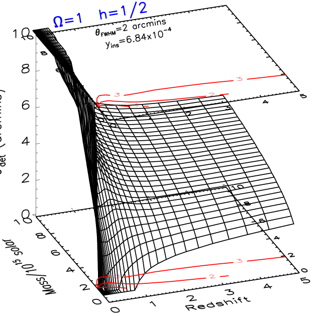
Figure 5: c) Source detection radius for $\theta_{\rm fwhm}=2$ arcmins and $\hat{y}=6.84\times 10^{-4}$, e.g., $\lambda=1$ cm and $q_{\rm st}\sigma_{\rm pix}=1.5$ mJy.

So far, nothing extraordinary, but rather the standard issues of extended object detection given a particular intensity profile. Modeling more specific to the SZ effect enters only when we apply the SZ–based relations between the central surface brightness and angular size – $y_{\rm o}$ and $\theta_{\rm c}$ – and the theoretically meaningful quantities of cluster mass, $M$, and redshift, $z$. These relations allow us to translate a surface like that of Figure 4 into an equivalent surface over the $(z,M)$–plane, as shown for three different cases in Figure 5 (all using our adopted self–similar cluster model). Note that these latter surfaces (Figure 5) are not uniquely parameterized by $\hat{y}$, because the translation from the axes in Figure 4 to mass and redshift explicitly involves $\sigma_{\rm b}$. Thus, there are now two governing parameters, which we can take to be $\hat{y}$ and $\sigma_{\rm b}$:

$$\theta_{\rm det}[z,M;\hat{y},\sigma_{\rm b}]$$

To study Figure 5 in detail, recall the simple scaling relations $y_{\rm o}\sim nM\sim M\Delta_{\rm NL}(z)(1+z)^{3}$ and $\theta_{\rm c}\sim M^{1/3}\Delta_{\rm NL}^{-1/3}(z)(1+z)^{-1}/D_{\rm ang}(z)$, valid if the core radius scales with virial radius (it may not, but this has been assumed in the construction of the figure). Notice that mass and redshift are mixed in a nontrivial way in the expressions for surface brightness and angular extent. In particular, a cluster of given mass becomes more centrally bright towards higher redshift, due to a higher gas density (scaling $\sim$ the background), while its angular extent at first decreases rapidly, as $\sim 1/z$ at low redshift, and then approaches an asymptote, since $(1+z)D_{\rm ang}(z)\rightarrow 2c(H_{\rm o}\Omega_{\rm o})^{-1}$ towards large $z$.

Consider firstly the low–redshift region of Figure 5b (the various effects are most clearly displayed in panel b), where the $z$-dependence is dominated by $D_{\rm ang}$; here, mass uniquely parameterizes the surface brightness, i.e., $y_{\rm o}$, while $z$ changes only $\theta_{\rm c}$:

• At constant $M$, decreasing $z$ increases the angular size of a cluster, so that, for resolved objects that are not completely below the surface brightness detection threshold ($q_{\rm st}\sigma_{\rm pix}/\Omega_{\rm pix}$), $\theta_{\rm det}$ rises as $1/z$; this corresponds to the $\theta_{\rm det}/\theta_{\rm c}\propto const$ behavior in Figure 4. For smaller objects, of low mass, the beam profile determines the scaling of $\theta_{\rm det}$ with $z$, and this corresponds to the point–source limit of Figure 4.

• At fixed (low) redshift, low mass objects eventually fall below the surface brightness limit, and $\theta_{\rm det}$ reaches zero; on the other hand, massive clusters are ‘lit–up’ out to their virial radius, at which point $\theta_{\rm det}$ attains $\theta_{\rm vir}=x_{\rm v}\theta_{\rm c}$, which grows as $M^{1/3}$.

An important aspect of detection procedure, mentioned at the beginning of this section and now evident from Figure 5, is the existence of a minimum detectable mass in the limit of zero redshift (on the $M$–axis). This characteristic mass is established by the surface brightness threshold – $q_{\rm st}\sigma_{\rm pix}/\Omega_{\rm pix}$, and its existence represents a fundamental difference with the previous case of optimal detection, where arbitrarily low mass (low surface brightness) clusters where picked up if they were large enough, i.e., very close at $z=0$. We already saw in Eq. (17) how $\hat{y}$ summarizes the surface brightness constraint. The low redshift detection mass limits seen in Figure 1 and here in Figure 5 are indeed reproduced numerically from Eq. (17), once Eq. (11) is used to convert $y_{\rm o}$ into a mass at $z=0$.

At redshifts approaching unity and beyond, $M$ and $z$ are fully mixed in the expressions for $y_{\rm o}$ and $\theta_{\rm c}$:

• Massive clusters well above the surface brightness threshold increase in surface brightness with redshift to the point where they are completely seen, all the way out to $\theta_{\rm vir}$; at even larger $z$, $\theta_{\rm det}$ reflects the gradual fall–off to the asymptote set by the angular–size distance. This explains the ridge running down the surface in Figure 5 around $z=1$. Less massive clusters, on the other hand, only reach the point of full illumination at higher $z$, well into the asymptotic behavior of $\theta_{\rm vir}$, and hence the ridge tends to be washed out at the low mass end. Finally, the central surface brightness of very low mass clusters falls below the detection threshold at ever larger redshifts, i.e., the boundary $\theta_{\rm det}=0$ moves outward in $z$ as $M$ is decreased.

Compare now the three panels of Figure 5. We observe the greater sensitivity at $2$ mm, due to the spectrum of the SZ effect, by the fact that a given cluster of mass $M$ and $z$ produces a smaller $\theta_{\rm det}$ at $1$ cm wavelength in panel b (notice the change in scale along the $M$–axis between panels a and b). The same remarque applies to the greater sensitivity, at a given noise level, of the lower resolution observations exemplified in panel c. These characteristics will be inherited by the detection mass curves, our next topic.

5.2.1 Detection mass as a function of redshift

Since $\theta_{\rm det}$ increases monotonically with $M$, the contours displayed on the top and bottom faces of Figure 5 represent curves of minimum detectable mass, $M_{\rm det}^{\rm st}(z;\theta_{\rm det})$, each one for a different detection threshold defined by different values of $\theta_{\rm det}$ (indicated in arcminutes on the contours in the figure). All of these contours, however, are defined for the same value of $q_{\rm st}\sigma_{\rm pix}$ set by the governing parameters $\hat{y}$ and $\sigma_{\rm b}$ (or $\theta_{\rm fwhm}$). In contrast to the optimal routine, a detection in the standard case is specified by not one, but two parameters – the pair $(q_{\rm st},\theta_{\rm det})$. This embodies the fact that a detection must satisfy two criteria: a minimum flux density, $\sim q_{\rm st}\sigma_{\rm pix}\theta_{\rm det}^{2}/\Omega_{\rm pix}$, and a minimum surface brightness, $\sim q_{\rm st}\sigma_{\rm pix}/\Omega_{\rm pix}$. In practice, the choice of values for $q_{\rm st}$ and $\theta_{\rm det}$ may be somewhat of a black art, but once made it specifies the survey’s characteristic $M_{\rm det}^{\rm st}(z)$. For the ensuing examples, I make the choice motivated by the following considerations: Note that the signal–to–noise of a detection $S/N=q_{\rm st}\sqrt{N_{\rm min}}$. The detection criteria imposed as $\theta_{\rm det}=\sqrt{N_{\rm min}}\theta_{\rm pix}$ may then be expressed in terms of the $S/N$:

$$\theta_{\rm det}=\frac{1}{q_{\rm st}}\left(\frac{S}{N}\right)\left(\frac{\theta_{\rm pix}}{\theta_{\rm fwhm}}\right)\theta_{\rm fwhm}$$ (18)

For reference, recall that in the optimal approach the parameter $q_{\rm opt}$ was exactly the $S/N$. Now, at fixed signal–to–noise, a larger $q_{\rm st}$ leads to a smaller $N_{\rm min}$ (i.e., $\theta_{\rm det}$), which facilitates the detection of fainter point sources, because their flux density is buried in less noise (fewer pixels). On the other hand, a large value of $q_{\rm st}$ disfavors finding low surface brightness objects; thus, a compromise is called for. One reasonable choice would be $\theta_{\rm det}=(1/2)\theta_{\rm fwhm}$, corresponding to a minimum detection $S/N\sim 3$, with $q_{\rm st}\sim 3$ and $\theta_{\rm pix}/\theta_{\rm fwhm}\sim 1/2$. I henceforth adopt these values for the following examples, which now completely specifies our detection routine.

The dot–dashed lines in Figure 1 show the resulting standard mass detection curves. They all lie above the optimal detection curves, implying a lower overall sensitivity, as expected; and as in the previous cases, they fall with $z$. The low resolution examples in Figure 1c show a slight turn–down at low redshift, but under no circumstances will they ever reach the origin at $z=0$, as do the unresolved and optimal resolved detection curves: as already mentioned, there always remains a non–zero detection mass at low $z$ in the standard case, due to the surface brightness cut. This constraint may be neatly summarized, using our earlier result, as $y_{\rm o}[M_{\rm det}^{\rm st}(z=0),0]=\hat{y}/2\pi$ (but it must be noted that this relies on our use of the self–similar cluster model). The loss of close–by, low–mass halos is particularly noteworthy for the study of low–mass halos; to find them in an SZ survey, one of the important potentials of such efforts, will require special “tuning” of detection criteria, to more closely approach the optimal routine.

5.2.2 Counts

Our next goal is to use the detection mass to calculate the cluster counts and redshift distributions. It is worth noting in passing that one can envision several different kinds of source counts: as a function of the value of $\theta_{\rm det}$, as a function of some aperture flux density (fixed or isophotal) or as a function of survey sensitivity, $\sigma_{\rm pix}$. Only the last one, however, is useful for optimizing an observing strategy, i.e., to answer the question of whether it is better to ‘go deep’, or to ’go wide’ when performing a survey. We are thus brought to consider in detail the detection mass as a function of detector sensitivity – $M_{\rm det}^{\rm st}(z;\sigma_{\rm pix})$. The most direct efficient way to do this for a large number of different sensitivities is by returning to Eq.(16), fixing $\theta_{\rm det}(=1/2\theta_{\rm fwhm})$ and then finding the detection mass as the root of the equation for each $z$. This avoids having to calculate the entire $\theta_{\rm det}$ surface for each $\sigma_{\rm pix}$ ($\hat{y}$) just to extract a single contour.

Using the result of this operation in Eq.(13), we find the counts and redshift distributions displayed in Figures 2 and 3 as the dot–dashed lines. Not surprisingly, the counts are lower at a given sensitivity than the corresponding optimal counts, and they are also slightly steeper. Similar remarks apply to the results of Figure 3. All of this is easily understood from the loss of low–surface brightness objects relative to the optimal routine. The essential conclusion concerning observation strategy remains the same: down to low flux densities, deeper integrations should yield more sources.

6 Discussion

The effects of resolving clusters must be properly modeled to understand the capabilities of possible ground–based surveys, as is clear from, for example, Figure 2: predicted counts are lower and steeper for resolved clusters relative to hypothetical SZ point sources. Besides lowering the expectations for the number of detectable sources, these results also suggest that deep integrations are more efficient than wide and shallow ones. The actual number of clusters expected for realistic ground–based performance are model dependent. For a self–similar cluster population, one could reasonably expect between 10–100 clusters/sq. deg. down to $0.1$ mJy at $2$ mm and with $\theta_{\rm fwhm}=1$ arcmin, as shown in Figure 2a. This number depends in addition on the source detection method employed: the standard routine counts may perhaps be considered realistic, while the optimal method counts indicate instead the best one could hope to achieve. At $1$ cm, for equivalent sensitivity and at the lower resolution of $\theta_{\rm fwhm}=2$ arcmin, one expects an order of magnitude lower surface density (Figure 1c). In sum, a square degree survey at $2$ mm could yield $\sim 10-100$ detections depending on the exact cluster model and the detection algorithm; a 10 square degree survey at $1$ cm to the same sensitivity ($0.1$ mJy) could produce similar numbers. Both types of survey may soon be achievable, with instruments similar to BOLOCAM (Glenn et al. 1998) or a detected interferometer array (Carlstrom et al. 1999)

One of the primary interests of opening this new window onto the Universe is to the search for high redshift clusters. The details of resolved cluster detection do not change the important and tell–tail difference between the redshift distributions in different cosmological models: the expected number of high redshift clusters is a sensitive function of $\Omega_{\rm o}$, as demonstrated by the redshift distributions given in Figure 3. Observations of such redshift distributions should prove a valuable tool for constraining $\Omega_{\rm o}$ and for understanding evolution of the cluster environment.

There are several important issues that have not been dealt with in the present work. One concerns eventual source confusion, an effect that depends on the beam size and the exact value of the counts. This effect may very well be important even on arcminute scales, as noted by Aghanim et al. (1997). As these authors also point out, the issue is complicated by the fact that, due to the extended nature of clusters, one must also contend with source blending. Detailed modeling of these effects really requires simulations.

Another important issue not addressed in the present work concerns the question of radio source contamination. With sufficient frequency coverage, on can always identify SZ sources by their unique spectrum. Most often, though, spectral coverage is limited and contamination may become problematic. Its importance depends on the observation frequency, and the counts at millimeter wavelengths are in fact a subject of current fundamental research; thus, the nature of contamination at in the millimeter is much more model dependent than in the centimeter.

Finally, I note once again that the present work is based on a simple cluster model, because the principal motivation has been to understand the nature of resolved cluster detection by comparison to the more classic unresolved case. Any attempt at a more exact examination of the number counts and redshift distributions requires more detailed cluster modeling. Such work would, in addition, permit an interesting comparison of the relative efficiencies of SZ and X–ray observations to finding high redshift clusters, in practice. The SZ effect is clearly inherently more efficient, but to really address this question, one should consider the actual achievable sensitivities of the two approaches.

7 Conclusions

There are clear and important differences in the conclusions one draws concerning SZ surveys depending on whether clusters are considered as point sources or as extended. For low resolution surveys, such as expected from the Planck Surveyor, most clusters will remain unresolved; however, when discussing the arcminute resolution more applicable to possible future ground–based surveys, we have seen that it is important to model the clusters as resolved sources in order to properly understand the nature of detectable objects. For a given sensitivity, high angular resolution “resolves out” some clusters, lowering and steepening the final source counts. Relative to optimal resolved detection, standard algorithms tend to in addition loose low mass, low redshift clusters due to their imposed surface brightness cut, further steepening and lowering the counts. With a fixed total observation time and a given frequency and angular resolution, we have seen that our results imply that deep integrations yield more objects than shallow ones covering a large area.

Some important issues still to be explored concern the questions of source confusion and blending, and radio source contamination. A detailed comparison of SZ and X–ray surveys would also be of interest, which implies more detailed cluster modeling than employed here.

All the same, the numbers from the self–similar cluster model should be, within all the present uncertainties of these predictions, illustrative of what may be soon achieved from the ground. It appears that both in the millimeter and in the cm, ground–based SZ surveys could be capable of detecting up to $\sim 100$ clusters in total, a respectable statistical catalog.

- (1) Aghanim N., de Luca A., Bouchet F.R., Gispert R. & Puget J.L. 1997, A&A 325, 9
- (2) Bahcall N. & Fan X. 1998, ApJ 504, 1
- (3) Barbosa D., Bartlett J.G., Blanchard A. & Oukbir J. 1996, A&A 314, 13
- (4) Bartlett J.G., Blanchard A. & Barbosa D. 1998, A&A 336, 425
- (5) Bartlett J.G. 1997, in: From Quantum Fluctuations to Cosmological Structures, School held in Casablanca, ed. D.Valls-Gabaud, M.A.Hendry, P.Molaro, K.Chamcham, A.S.P. Conf. Ser., vol. 126, p 365
- (6) Bartlett J.G. & Silk J. 1994, ApJ 423, 12
- (7) Bertin E. & Arnouts S. 1996, A&A Supp. 117, 393
- (8) Blanchard A., Sadat, R., Bartlett J.G. & Le Dour M. 1999, astro–ph/9908037
- (9) Bond J.R. & Meyers S.T. 1991, in: Trends in Astroparticle Physics, ed. D. Cline, World Scientific, Singapore
- (10) Borgani S., Rosati P., Tozzi P. & Colin N. 1999, ApJ 517, 40
- (11) Bryan G.L. & Norman M.L. 1998, ApJ 495, 80
- (12) Carlstrom J.E., Joy M. & Grego L. 1996, ApJL 456, L75
- (13) Carlstrom J.E., Joy M.K., Grego L., Holder G.P., Holzapfel W.L., Mohr J.J., Patel S. & Reese E.D. 1999, astro–ph/9905255
- (14) Challinor A. & Lasenby A. 1998, ApJ 499, 1
- (15) Colafrancesco S. & Vittorio N. 1994, ApJ 422, 443
- (16) Colafrancesco S., Mazzotta P., Rephaeli Y. & Vittorio N. 1997, ApJ 433, 454
- (17) Eke V.R., Cole S. & Frenk C.S. 1996, MNRAS 282, 263
- (18) Eke V.R., Cole S., Frenk C.S. & Henry P.J. 1998, MNRAS 298, 1145
- (19) Elbaz D., Arnaud M. & Vangioni–Flam E. 1995, A&A 303, 345
- (20) Evrard A.E., Metzler C.A. & Navarro J.F. 1996, ApJ 469, 494.
- (21) Evrard A.E. 1997, MNRAS 292, 289
- (22) Glenn J., Bock J.J., Chattopadhyay G. et al. 1998, SPIE Conference on Advanced Technology Millimeter-Wave, Radio, and Terahertz Telescopes, Vol. 3357, p. 326
- (23) Henry J.P. 1997, ApJ 489, L1
- (24) Holder G.P. & Carlstrom J.E. 1999, astro–ph/9904220
- (25) Holder G.P., Mohr J.J., Carlstrom J.E., Evrard A.E. & Leitch E.M. 1999, astro–ph/9912364
- (26) Itoh N., Kohyama Y. & Nozawa S. 1998, ApJ 502, 7
- (27) Korolyov V.A., Sunyaev R.A. & Yakubtsev L.A. 1986, Sov. Astron. Lett. 12, L141
- (28) Lacey C. & Cole S. 1994, MNRAS 271, 676
- (29) Markevitch M., Blumenthal G.R., Forman W., Jones C. & Sunyaev R.A. 1994, ApJ 426, 1
- (30) Mather J.C., Fixsen D.J., Shafer R.A., Mosier C. & Wilkinson D.T. 1999, ApJ 512, 511
- (31) Metzler C.A. & Evrard A.E. 1994, ApJ 437, 564
- (32) Mohr J.J., Mathiesen B. & Evrard A.E. 1998, ApJ 517, 627
- (33) Mohr J.J., Carlstrom J.E. & Holder G.P. et al. 1999, astro–ph/9905256
- (34) Oukbir J. & Blanchard A. 1992, A&A 262, L21
- (35) Oukbir J. & Blanchard A. 1997, A&A 317, 1
- (36) Pointecouteau E., Giard M. & Barret D. 1998, A&A 336, 44
- (37) Press W.H. & Schechter P. 1974, ApJ 187, 425
- (38) Rephaeli Y. 1995, ApJ 445, 33
- (39) Sazonov S.Y. & Sunyaev R.A. 1998, ApJ 508, 1
- (40) Stebbins A. 1997, ApJ submitted, astro–ph/9709065
- (41) Viana P.T.P. & Liddle A.R. 1999a, MNRAS 303, 535
- (42) Viana P.T.P. & Liddle A.R. 1999b, astro-ph/9902245
- (43) White S.D.M., Navarro J.F., Evrard A.E. & Frenk C.S. 1993, Nature 366, 429
- (44) Sunyaev R.A. & Zel’dovich Ya.B. 1972, Comm. Astrophys. Space Phys. 4, 173