On the numerical analysis of triplet pair production cross-sections and the mean energy of produced particles for modelling electron-photon cascade in a soft photon field

Abstract

The double and single differential cross-sections with respect to positron and electron energies as well as the total cross-section of triplet production in the laboratory frame are calculated numerically in order to develop a Monte Carlo code for modelling electron-photon cascades in a soft photon field. To avoid numerical integration irregularities of the integrands, which are inherent to problems of this type, we have used suitable substitutions in combination with a modern powerful program code (Mathematica) allowing one to achieve reliable higher-precission results. The results obtained for the total cross-section closely agree with others estimated analytically or by a different numerical approach. The results for the double and single differential cross-sections turn out to be somewhat different from some reported recently. The mean energy of the produced particles, as a function of the characteristic collisional parameter (the electron rest frame photon energy), is calculated and approximated by an analytical expression that revises other known approximations over a wide range of values of the argument. The primary-electron energy loss rate due to triplet pair production is shown to prevail over the inverse Compton scattering loss rate at several ($\sim$2) orders of magnitude higher interaction energy than that predicted formerly.

Published in Journal of Physics G: Nuclear and Particle Physics. Copyright 1999 IOP Publishing Ltd

1 Introduction

There are two main reasons why triplet pair production (TPP) has been commonly ignored in astrophysical applications. The first reason is that TPP is a third-order QED process. The second reason is the extremely complicated and long expression for the total differential cross-section [1]. This considerably complicates the modelling of the energies and momenta of the final three particles in comparison with the case of considering only the two major processes for electron-photon cascade in a radiation field: pair production and inverse Compton scattering. Apart from the formal complications there are serious mathematical problems to be overcome connected with numerical calculation of the double differential cross-section (DDCS) and single differential cross-section (SDCS) in the laboratory frame. A typical problem is the integration over the cosine ($\cos\theta_{-}$) of the polar angle $\theta_{-}$ of the produced electron momentum $p_{-}$, where both the integrand irregularities coincide with the integration limits whose semi-vicinities provide the major contribution to the integral.

Despite the above-mentioned arguments, at ultrarelativistic electron energies TPP becomes a prevailing process playing an important part in the electron-photon cascades in a soft background photon field that form the energy spectrum from a variety of astrophysical sources. This fact has been recently emphasized and confirmed by incorporating TPP into full cascade calculations [2]-[5].

Based on the recently revived interest in a more precise simulation of electron-photon cascades in a photon field, we have started to develop a Monte Carlo code for modelling TPP. Our intention is to use this code for a more detailed study of the development of electromagnetic cascades in thermal fields. To realize this intention we have decided to follow a method like that suggested in paper [4]. Thus, as an initial step we have precisely recalculated the DDCS and SDCS with respect to electron and positron energies as well as the total cross-section of TPP in the laboratory frame. An obstacle to overcome here is the presence of the above-mentioned integrand irregularities in combination with extremely short integration intervals. So, one purpose of the present study is to search for ways to avoid these intrinsic difficulties and to achieve more precise results. Another purpose of the study is to calculate and analytically approximate the mean energy of particles produced as a function of the characteristic collisional parameter. Investigating the primary-electron TPP energy loss rate is also an important aim of the work.

2 Method and results

2.1 Calculation approach

Let us first consider the basic expressions of interest corrected [6] for typographical errors that have appeared in many papers. The DDCS with respect to the positron and electron energies is given by

$$\frac{\rmd^{2}\sigma}{\rmd E_{+}\rmd E_{-}}(E_{0},\varepsilon_{0},s,E_{+},E_{-})$$

$$\hbox to0.0pt{\hss${}={}$}\frac{\alpha_{f}\,r_{0}^{2}}{4\pi^{2}s}p_{+}p_{-}\int_{x_{\min}}^{1}\rmd x\int_{y_{\min}(x)}^{y_{\max}(x)}\rmd y[a_{1}(y_{\max}-y)(y-y_{\min})]^{-1/2}\int_{0}^{2\pi}X\rmd\phi_{+},$$ (1)

where $p_{+}$, $E_{+}$, $\theta_{+}$ and $p_{-}$, $E_{-}$, $\theta_{-}$ are momenta, energies and polar angles of the produced positron and electron, respectively, $x=\cos\theta_{+}$ and $y=\cos\theta_{-}$, $\phi_{+}$ is the azimuthal angle of the positron, $E_{0}$ and $\varepsilon_{0}$ are the energies of the incoming electron and photon respectively, $s=E_{0}\varepsilon_{0}(1-\beta\cos\theta)$ is the characteristic collisional parameter ($\theta$ is the collision angle) representing the photon energy in the electron rest frame (ERF), and $X$ is a cumbersome expression that is given in the appendix; the quantities $\alpha_{f}=e^{2}/(\hbar c)$ and $r_{0}=e^{2}/(m_{e}c^{2})$ are the fine structure constant and the classical electron radius, respectively, and $m_{e}$ is the electron rest mass. The limits of integration are:

Figure 1: Integrand function $X(E_{0},\varepsilon_{0},s,E_{+},E_{-},x,y,\phi_{+})[a_{1}(y_{\max}-y)(y-y_{\min})]^{-1/2}$ in arbitrary units (before change of variables) versus the polar-angle cosine $y=\cos\theta_{-}$ at $E_{0}=10^{8}$, $\varepsilon_{0}=10^{-3}$, $s=10^{5}$, $E_{+}=4.999925000425\times 10^{7}$, $E_{-}=2.500037499837\times 10^{7}$, $x=\cos\theta_{+}=0.999999999995$, $\phi_{+}=\pi$.

$$y_{\max}=[b_{1}+(b_{1}^{2}-a_{1}c_{1})^{1/2}]/a_{1},$$

$$y_{\min}=[b_{1}-(b_{1}^{2}-a_{1}c_{1})^{1/2}]/a_{1},$$

$$x_{\min}=-(F_{1}+p_{-}F_{2}^{1/2})/(p_{+}P_{tot}),$$

where

$$a_{1}=p_{-}^{2}(P_{tot}^{2}+p_{+}^{2}-2P_{tot}p_{+}x),\qquad b_{1}=Ap_{-}(p_{+}x-P_{tot}),$$

$$c_{1}=A^{2}-p_{+}^{2}p_{-}^{2}\sin^{2}\theta_{+},$$

$$A=1+s+p_{+}P_{tot}x-E_{tot}(E_{+}+E_{-})+E_{+}E_{-},$$

$$F_{1}=E_{-}^{2}-(E_{tot}-E_{+})E_{-}+s-E_{tot}E_{+},$$

$$F_{2}=(E_{+}+E_{-}-E_{tot})^{2}-1,\qquad E_{tot}=E_{0}+\varepsilon_{0},\qquad\mathrm{and}\qquad\overrightarrow{P}_{tot}=\overrightarrow{p}_{0}+\overrightarrow{k}.$$

$\overrightarrow{p}_{0}$ and $\overrightarrow{k}$are the momenta of the incoming electron and photon, respectively. Let us note that throughout this paper the energy quantities are in units $m_{e}c^{2}$. Note that the integrand in equation (1) has two irregular points with respect to the variable $y$. These points, $y=y_{\min}$ and $y=y_{\max}$, coincide with the integration limits. Also, the integration intervals over $x$ and $y$, especially at high energies, are extremely short. In addition, even within such narrow integration intervals the integrand changes sharply with changing of $y$ (see figure 1). Because of these peculiarities of the integrand, an accurate calculation (numerical integration) can be successful only when a sufficiently high-precision number is used. This was first been pointed out by Mastichiadis [4] who underlined the necessity of quadratic precision to calculate DDCS and SDCS, and reconsidered his own formerly obtained results [2]. Since our purpose here is to perform similar calculations with a higher precision (e.g. up to 80 significant decimal digits) we have used the program code Mathematica [7], which allows one to work with arbitrary high-precision numbers. Thus, one can both eliminate the precision number conditioning and ensure a reliable precision of the final results. In addition, this code has an adaptive program for quadrature of multiple integrals that precisely approximates the fast-changing integrand and permits one to obtain results with a prescribed precision. Nevertheless, the extraordinary character of the integrand in equation (1) leads to a fast growth of the CPU time with the increase of the interaction energies. Besides, it is not unknown for the program to fail in some cases. As a result of searching for ways to eliminate the above-mentioned problems, we came to the following change of variables that led to acceptable integration intervals and acceptable smooth behaviour of the integrand:

Figure 2: Integrand function $2X(E_{0},$$\varepsilon_{0},s,$$E_{+},E_{-},x,\eta,\phi_{+})/(1+\eta^{2})$ in arbitrary units (after change of variable $y$) versus the new variable $\eta$ at the same fixed values of the remaining variables as in figure 1.

$$x = x(\xi)=\xi/l+x_{\min}\quad(l>1),$$ (2a)

$$y = y(\xi,\eta)=[y_{\max}(x)+y_{\min}(x)\eta^{2}]/(1+\eta^{2}){.}$$ (2b)

Equation (2b) is, in fact, one of the Euler substitutions that is appropriate for this case and leads to the integral:

$$I=I(E_{0},\varepsilon_{0},s,E_{+},E_{-})=2l^{-1}\int_{0}^{l(1-x_{\min})}\rmd\xi\int_{0}^{\infty}\rmd\eta$$

$$\hbox to0.0pt{\hss${}\times{}$}\int_{0}^{2\pi}\rmd\phi_{+}X(E_{0},\varepsilon_{0},s,E_{+},E_{-},\xi,\eta,\phi_{+})/(1+\eta^{2}){;}$$ (2c)

$$\rmd^{2}\sigma/(\rmd E_{+}\rmd E_{-})=(\alpha_{f}\,r_{0}^{2}/(4\pi^{2}a_{1}^{1/2}s))p_{+}p_{-}I(E_{0},\varepsilon_{0},s,E_{+},E_{-}){.}$$

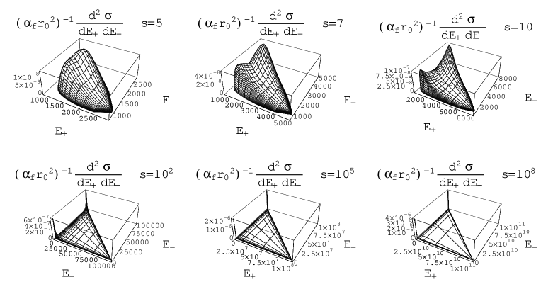
Figure 3: DDCS $(\alpha_{f}r_{0}^{2})^{-1}\rmd^{2}\sigma/(\rmd E_{+}\rmd E_{-})$ as a function of $E_{+}$ and $E_{-}$ at various values of $s$; $\varepsilon_{0}=10^{-3}$, $E_{0}=s/\varepsilon_{0}$ (glancing collision).

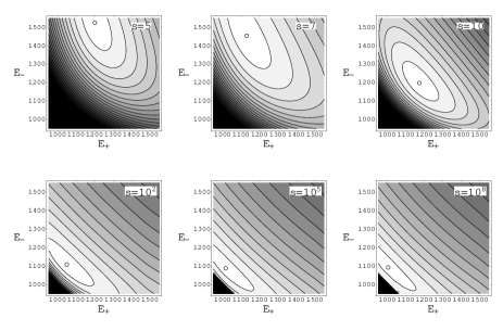
Figure 4: Three-dimensional contour plot of $(\alpha_{f}r_{0}^{2})^{-1}\rmd^{2}\sigma/(\rmd E_{+}\rmd E_{-})$ as a function of $E_{+}$ and $E_{-}$, at values of $s$ as in figure 3, respectively, around the first peak of figure 3 disposed near $E_{+,\min}$ and $E_{-,\min}$; $\varepsilon_{0}=10^{-3}$, $E_{0}=s/\varepsilon_{0}$ (glancing collision).

It can be seen that the new variables lead to an enlargement of the integration scale and removal of the integrand irregularities. As one may expect, the integrand becomes a smooth function of $\eta$ (figure 2), which leads to an acceleration of the calculation procedure, increase of the precision, and elimination of any computational failures when Mathematica is used.

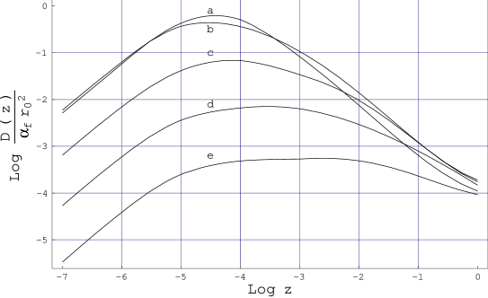
Figure 5: Dependence of the quantity $(\alpha_{f}r_{0}^{2})^{-1}D(s,z)=(E_{-}-E_{-,\min})(E_{+}-E_{+,\min})[\rmd^{2}\sigma/(\rmd E_{+}\rmd E_{-})]$ on the parameter $z=(E_{-}-E_{-,\min})/(E_{-,med}-E_{-,\min})$ [$E_{-,med}=0.5(E_{-,\min}+E_{-,\max})$] for $E_{-,\min}<E_{-}<E_{-,med}$ and various outgoing positron energies $E_{+}=10^{3}$($a$),$10^{4}$($b$),$10^{5}$($c$),$10^{6}$($d$) and $10^{7}$($e$); $E_{0}=10^{8}$ and $\varepsilon_{0}=10^{-3}$ ($s=10^{5}$).

2.2 Double differential cross-section

We have obtained precise results for DDCS as a function of $E_{0}$, $\varepsilon_{0}$, $s$, $E_{+}$ and $E_{-}$. Some of these results are shown in figures 3 and 4 in a three-dimensional surface form and a three-dimensional contour form, respectively. It is seen (figure 3) that the dependence of $\rmd^{2}\sigma/(\rmd E_{+}\rmd E_{-})$ on $E_{+}$ and $E_{-}$ considered over the whole range of the arguments $E_{+}$ and $E_{-}$, at various fixed values of the parameter $s=\varepsilon_{0}E_{0}$ ( in the case of a glancing collision when $\theta=\pi/2$ ), is represented by a double-peak surface whose secants with the planes $E_{+}=const$ are symmetric curves with respect to the point $(E_{+},E_{-,med})$, where $E_{-,med}=0.5(E_{-,\min}+E_{-,\max})$. With the increase of $s$, the surface peak heights increase, and the surface itself (as well as the corresponding dependence of DDCS on $E_{+}$ and $E_{-}$) becomes sharper. Also, up to values of $s=10^{2}$, the peaks change their positions over the plane $\{E_{+},E_{-}\}$. So, the common coordinate of both peaks along $E_{+}$ axis is shifted to lower values of $E_{+}$. In addition, the first peak (disposed below the point $(E_{+},E_{-,med})$) is shifted to lower values of $E_{-}$ (see figure 4), and the second one, to higher values of $E_{-}$. At values of $s$ increasing above $s=10^{2}$ the peaks do not change their positions; the surface is as if consisting of two spikes (with a common $E_{+}$ coordinate) whose positions are close to the points $(E_{+,\min},E_{-,\min})$ and $(E_{+,\min},E_{-,\max})$, respectively. The same results as above are represented in figure 5, but in a parametrized form proposed in [4], where the quantity $D(s,z)=(E_{-}-E_{-,\min})(E_{+}-E_{+,\min})[\rmd^{2}\sigma/(\rmd E_{+}\rmd E_{-})]$ is considered as a function of the parameter $z=(E_{-}-E_{-,\min})/(E_{-,med}-E_{-,\min})$ at fixed values of $E_{+}$ and $s$. It is shown in [4] that $D$ can be considered as dependent only on $s$ and $z$ if $E_{0}\gg 1\gg\varepsilon_{0}$. Such a parametrization is useful for application to a Monte Carlo code for modelling electron-photon cascades in a soft photon field taking into account the contribution of the TPP process. Then, on the basis of tabulated data $D(s,z)$ one can determine DDCS at any combination of $E_{0}$, $\varepsilon_{0}$, $s$ and positron energy $E_{+}$ [4]. Comparison between our results and those obtained in [4] shows that our curves pass through maximum and that at lower electron energies tending to $E_{-,\min}$, where the calculation is sensitive to loss of precision, they essentially fall below the corresponding curves obtained in [4].

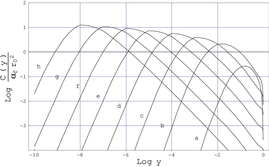
Figure 6: Dependence of the quantity $(\alpha_{f}r_{0}^{2})^{-1}C(s,y)=(E_{+}-E_{+,\min})[\rmd\sigma/\rmd E_{+}]$ on the parameter $y=(E_{+}-E_{+,\min})/(E_{+,\max}-E_{+,\min})$ for various ERF energies of collision $s=10$($a$),$10^{2}$($b$),$10^{3}$($c$),$10^{4}$($d$),$10^{5}$($e$),$10^{6}$($f$),$10^{7}$($g$) and $10^{8}$($h$).

Table 1: TPP total cross-sections (in units $\alpha_{f}\,r_{0}^{2}$).

• $s,s_{\perp}$	$\sigma_{tot,Haug}$	$\sigma_{tot,Mast}$	$\sigma_{tot,Our}$	$\sigma_{toti,Our}$
  4.01	$5.80\times 10^{-7}$	$5.4\times 10^{-7}$	$5.8\times 10^{-7}$	0.092
  4.1	$7.53\times 10^{-5}$	$7.6\times 10^{-5}$	$7.5\times 10^{-5}$	0.102
  5	0.0170	0.019	0.0170	0.221
  7	0.179	0.19	0.179	0.56
  10	0.594	0.59	0.59	1.12
  $10^{2}$	7.21	7.3	7.3	7.9
  $10^{3}$	15.1	15.3	15.1	15.8
  $10^{4}$	22.6	22.4	22.7	23.2
  $10^{5}$	29.9	29.7	29.9	30.5
  $10^{6}$	37.1	37.0	37.	38.
  $10^{7}$	44.2	-	44.	45.
  $10^{8}$	51.4	-	52.	52.

2.3 Single differential cross-section

The SDCS $\rmd\sigma/\rmd E_{+}$ has been calculated by integrating $\rmd^{2}\sigma/(\rmd E_{+}\rmd E_{-})$ over $E_{-}$ with integration limits $E_{\_}|_{\min}^{\max}=0.5[E_{tot}-E_{+}\pm(P_{tot}-p_{+})(1-2/B)^{1/2}]$, $(B=1+s-E_{tot}E_{+}+P_{tot}p_{+})$. In the same way, $\rmd\sigma/\rmd E_{-}$ has been calculated by integrating $\rmd^{2}\sigma/(\rmd E_{+}\rmd E_{-})$ over $E_{+}$. The use of an optimum-power spline technique allowed us to obtain precise results for sufficiently high values of $s>10^{8}$. (We consider as an optimum power of the spline that one, above which the results from the integration remain stable.) The same results have been obtained by direct integration (without spline interpolation) but using considerably longer CPU time. Some of the results obtained are shown in figure 6 in a parametrized form where the quantity $C(s,y)=(E_{+}-E_{+,\min})[\rmd\sigma/\rmd E_{+}]$ is considered as a function of the parameter $y=(E_{+}-E_{+,\min})/(E_{+,\max}-E_{+,\min})$ at fixed values of $s$. For $E_{0}\gg 1\gg\varepsilon_{0}$, $C(s,y)$ depends only on $s$ and $y$, and (when tabulated) allows one to determine the SDCS for any combination of $E_{0}$, $\varepsilon_{0}$ and $s$ [4]. The comparison between our results and those obtained in [4] shows that the corresponding curves have the same behaviour with a characteristic maximum. The difference is that the left-hand part of each curve of ours (including the maximum), where the calculation is more sensitive to loss of precision, is as if shifted right with respect to the analogous part of the corresponding curve obtained in [4].

2.4 Total cross-section

We have also calculated the total cross-section $\sigma_{tot}$ by integrating $\rmd\sigma/\rmd E_{+}$ over $E_{+}$. The integration limits are: $E_{+}|_{\min}^{\max}=\{E_{tot}(s-1)\pm P_{tot}[s(s-4)]^{1/2}\}/(1+2s)$ [4]. The results obtained are compared, in table 1, with the results obtained by other authors [4], [8]. The agreement is excellent and may be considered as an indirect confirmation of the precise character of our calculations.

2.5 Mean energy of produced particles

Finally, we have calculated the mean energy $E_{m}=E_{+,m}=E_{-,m}$ of the produced particles on the basis of the relations:

$$E_{m} = E_{+,-,m}=\int E_{+,-}(\rmd\sigma/\rmd E_{+,-})\rmd E_{+,-}/\sigma_{tot}$$ (2d)

The results obtained for $E_{+,m}$ and $E_{-,m}$ are practically coincident, which may be considered as another confirmation of the precise character of the calculations performed. On the basis of the parametrization approach developed in [4] we can show that the ratio $E_{m}/E_{0}$ is a function only of $s$ when $E_{0}\gg 1\gg\varepsilon_{0}$. In this case, the integration limits $E_{+,\min}$ and $E_{+,\max}$ (see above) are expressible as $E_{+,\min}=E_{0}f_{\min}(s)$ and $E_{+,\max}=E_{0}f_{\max}(s)$, where the functions $f_{\min}$ and $f_{\max}$ depend only on $s$. After the change of variable $E_{+}=xE_{0}$, instead of equation (2d) we can write:

$$E_{m} = E_{0}\sigma_{tot}^{-1}(s)\int_{f_{\min}(s)}^{f_{\max}(s)}\rmd x.x.[(\rmd\sigma/\rmd x)(E_{0},\varepsilon_{0},s,xE_{0})]{.}$$ (2e)

In the same way, taking into account that $\sigma_{tot}$ depends only on $s$, we obtain

$$\sigma_{tot}(s)=\int_{f_{\min}(s)}^{f_{\max}(s)}\rmd x[(\rmd\sigma/\rmd x)(E_{0},\varepsilon_{0},s,xE_{0})]=\int_{f_{\min}(s)}^{f_{\max}(s)}\rmd x[(\rmd\sigma/\rmd x)(E_{0}^{{}^{\prime}},\varepsilon_{0}^{\prime},s,xE_{0}^{\prime})]$$ (2f)

where $E_{0}^{{}^{\prime}}$ and $\varepsilon_{0}^{\prime}$ are some other values of the incoming electron and photon energies, respectively, but such that the value of $s$ is retained. Based on equation (2f) we may conclude that $(\rmd\sigma/\rmd x)(E_{0}^{{}^{\prime}},\varepsilon_{0}^{\prime},s,xE_{0}^{\prime})=(\rmd\sigma/\rmd x)(E_{0},\varepsilon_{0},s,xE_{0})$, and consequently (see equation (2e)) $E_{m}/E_{0}=E_{m}^{{}^{\prime}}/E_{0}^{{}^{\prime}}=f(s)$, where

$$f(s) = \sigma_{tot}^{-1}(s)N(s){,}$$ (2g)

and

$$N(s)=\int_{f_{\min}(s)}^{f_{\max}(s)}\rmd x.x.[(\rmd\sigma/\rmd x)(E_{0},\varepsilon_{0},s,xE_{0})]{.}$$ (2h)

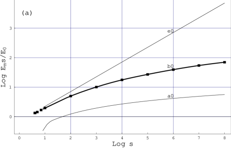
Figure 7: (a) Plot of the quantity $f_{1}(s)=E_{m}s/E_{0}$ (the mean energy $E_{m}$ of produced particles normalized to $E_{0}/s$) versus ERF collision energy $s$. The black squares represent the results from our calculations fitted by a cubic spline (curve($b_{0}$)); at $s>10^{2}$ curve ($b_{0}$) is well described by the function $f_{1}(s)=0.195\ln^{2}(2s)$. Curves ($e_{0}$) and ($a_{0}$) correspond to the approximation $f_{1}(s)=0.71s^{1/2}$ and $f_{1}(s)=\ln^{2}(s/4)/\sigma_{totBH}$ based on the results of Dermer and Schlickeiser [9], and Feenberg and Primakoff [10], respectively. (b) Plot of the quantity $\varphi_{1}(s_{\perp})=E_{mi}s_{\perp}/E_{0}=E_{mi}\varepsilon_{0}$ (the mean energy of produced particles in an isotropic and monochromatic soft photon field, $E_{mi}$, normalized to $E_{0}/s_{\perp}$) versus $s_{\perp}=\varepsilon_{0}E_{0}$. The black circles represent the results from our calculations. At $s_{\perp}\geq 10^{2}$ they are fitted by the function $\varphi_{1}(s_{\perp})=0.195\ln^{2}(2s_{\perp})$ represented by curve ($b_{1}$). Curves ($e_{1}$), ($d_{1}$), ($c_{1}$) and ($a_{1}$) correspond to the approximations $\varphi_{1}(s_{\perp})=\frac{2}{3}s_{\perp}^{1/2}$, $\varphi_{1}(s_{\perp})=0.57s_{\perp}^{0.44}$, $\varphi_{1}(s_{\perp})=2.5s_{\perp}^{0.25}$, and $\varphi_{1}(s_{\perp})=\varphi_{FP}(s_{\perp})$ based on the results of Dermer and Schlickeiser [9], Mastichiadis et al [2], Mastichiadis et al [4] and Feenberg and Primakoff [10], respectively.

Thus, the knowledge of $f(s)$ allows one to determine $E_{m}$ for any pair of values of $E_{0}$ and $s$. At fixed values of $E_{0}$ and $\varepsilon_{0}$, $f(s)$ describes, in practice the dependence of $E_{m}$ on the angle of collision $\theta$.

The results calculated for $E_{m}s/E_{0}$ versus $s$ are represented in figure 7(a) by black squares (see also table 2). At $s>10^{2}$ they are well described by the dependence (curve ($b_{0}$)):

Table 2: Normalized mean energies of produced particles.

• $s,s_{\perp}$	$E_{m}s/E_{0}$	$E_{mi}s_{\perp}/E_{0}=E_{mi}\varepsilon_{0}$	$0.195\ln^{2}(2s_{\perp})$
  4.01	1.337	1.69	0.84
  4.1	1.339	1.70	0.86
  5	1.44	1.84	1.03
  7	1.68	2.10	1.36
  10	1.97	2.39	1.75
  $10^{2}$	5.00	5.50	5.47
  $10^{3}$	10.1	10.7	11.3
  $10^{4}$	17.7	18.5	19.1
  $10^{5}$	27.1	28.2	29.0
  $10^{6}$	39.4	40.8	41.0
  $10^{7}$	54.2	55.8	55.1
  $10^{8}$	70.0	71.5	71.2

$$f_{1}(s) = E_{m}(E_{0},s)s/E_{0}=0.195\ln^{2}(2s)$$ (2i)

The concrete calculations are performed at $\varepsilon_{0}=10^{-3}$, $\theta=\pi/2$, and various values of $E_{0}$ leading to various values of $s=\varepsilon_{0}E_{0}$. Nevertheless, the results obtained for $E_{m}/E_{0}$ should, as a whole, depend only on $s$ independently of the concrete values of $E_{0}$, $\varepsilon_{0}$ and $\theta$. Thus, on the basis of a special case we obtain the dependence $E_{m}(E_{0},s)$ having a more general validity. In figure 7(a) we have also graphically represented two other estimates of the function $f_{1}(s)=E_{m}(E_{0},s)s/E_{0}$ obtained by other authors. The line ($e_{0}$) corresponds to the estimate $E_{m}(E_{0},s)=0.71E_{0}s^{-0.5}$obtained analytically by Dermer and Schlickeiser [9]. At values of $s\leq 10^{2}$ this line passes through our points (squares). At values of $s>10^{2}$ the line goes far above our points, thus predicting several orders of magnitude higher results for $E_{m}$. The curve ($a_{0}$) corresponds to the estimate $E_{m}(E_{0},s)=(E_{0}/s)\ln^{2}(s/4)/\sigma_{totBH}(s)$ obtained on the basis of the theoretical approach developed by Feenberg and Primakoff [10] (see equations (19), (21), (22) and (31) in [10]); $\sigma_{totBH}(s)$ is an analytical approximation to the Bethe-Heitler formula for $\sigma_{tot}(s)$ normalized to the quantity $\alpha_{f}r_{0}^{2}$. It is seen that curve ($a_{0}$) lies essentially below our points and predicts several times lower results for $E_{m}(E_{0},s)$. A reason for this is that curve ($a_{0}$) describes an approximation obtained analytically as a lower limit of the true dependence $f_{1}(s)$. Another reason, that was pointed out by Mastichiadis et al [2] is the neglect (in [10]) of the recoil of the primary electron in the electron rest frame.

In order to determine the mean energy $E_{mi}$ of a particle produced by relativistic electron-photon collision in an isotropic and monochromatic soft photon field one should additionally average $E_{m}$ over the angle of collision $\theta$. Then the expression of $E_{mi}$ is obtained in the form:

$$E_{mi}(E_{0},s_{\perp}) = E_{0}\varphi(s_{\perp}){,}$$ (2j)

where $\varphi(s_{\perp})=N_{i}(s_{\perp})/\sigma_{toti}(s_{\perp})$ is a function of $s_{\perp}=\varepsilon_{0}E_{0}$;

$$N_{i}(s_{\perp}) = (2\beta\varepsilon_{0}^{2}E_{0}^{2})^{-1}\int_{4}^{\varepsilon_{0}E_{0}(1+\beta)}sN(s)\rmd s{,}$$ (2k)

$$\sigma_{toti}(s_{\perp}) = (2\beta\varepsilon_{0}^{2}E_{0}^{2})^{-1}\int_{4}^{\varepsilon_{0}E_{0}(1+\beta)}s\sigma_{tot}(s)\rmd s{.}$$ (2l)

The results calculated for $\varphi_{1}(s_{\perp})=E_{mi}(E_{0},s_{\perp})s_{\perp}/E_{0}=E_{mi}(E_{0},s_{\perp})\varepsilon_{0}$ versus $s_{\perp}$ are represented in figure 7(b) by black circles (see also table 2). At $s_{\perp}\geq 10^{2}$ they are fitted by the dependence (curve ($b_{1}$))

$$\varphi_{1}(s_{\perp}) = E_{mi}(E_{0},s_{\perp})\varepsilon_{0}=0.195\ln^{2}(2s_{\perp})$$ (2m)

(i.e. $E_{mi}(E_{0},s_{\perp})\rightarrow E_{mi}(\varepsilon_{0},s_{\perp})=(0.195/\varepsilon_{0})\ln^{2}(2s_{\perp})$) that has the same form as the dependence $f_{1}(s)$ (equation (2i)). There are four more curves represented in figure 7(b), which describe some approximations of the function $\varphi_{1}(s_{\perp})$ obtained by different authors. The line ($e_{1}$) corresponds to the estimate $\varphi_{1}(s_{\perp})=\frac{2}{3}s_{\perp}^{1/2}$ [9]. Certainly, it almost coincides with the line ($e_{0}$) in figure 7(a), and at $s<10$ passes in immediate proximity to our points (circles). With the increase of $s_{\perp}$ above $10^{2}$, the discrepancy with our results also increases, achieving two orders of magnitude at $s=10^{8}$. The lines ($d_{1}$) and ($c_{1}$) correspond to the approximations $\varphi_{1}(s_{\perp})=0.57s_{\perp}^{0.44}$ and $\varphi_{1}(s_{\perp})=2.5s_{\perp}^{0.25}$ obtained by Mastichiadis et al in 1986 [2] and 1991 [4], respectively. The first approximation (line ($d_{1}$)) has been obtained by numerical calculations. It is near that obtained by Dermer and Schlickeiser, and has a similar behaviour with respect to our results. The latter approximation is obtained after reconsidering the first one and performing improved calculations and computer simulations. In the interval from $s=10^{3}$ to $s=10^{8}$ the line ($c_{1}$) lies just above our results. For completeness, we shall also briefly consider the results for $\varphi_{1}(s_{\perp})=\varphi_{FP}(s_{\perp})=(1/s_{\perp})\{s_{\perp}[(\ln s_{\perp}-\ln 2-1)^{2}+1]-[(\ln 2+1)^{2}+1]\}/\sigma_{totiFP}$ obtained on the basis of the approach of Feenberg and Primakoff (curve ($a_{1}$)) by using the above-mentioned equations (19), (21), (22) and (31) in [10]; $\sigma_{totiFP}$ is derived from equations (19) and (21) in [10], and is normalized to (divided by) $\alpha_{f}r_{0}^{2}$. The corresponding curve (($a_{1}$) in figure 7(b)) almost coincides with the curve ($a_{0}$) in figure 7(a), thus showing the same behaviour with respect to our results. The reasons for such a behaviour are pointed out above. The resemblance between our results and those of Feenberg and Primakoff is that $\varphi_{1}(s_{\perp})$ ($f_{1}(s)$) is obtained to be proportional to $\ln^{2}s_{\perp}$ and $\ln\,s_{\perp}$ ($\ln^{2}s$ and $\ln\,s$) respectively, and not to a power function of $s_{\perp}$ ($s$) as in the other known approximations. Let us finally note that the lowest estimate of $E_{m}\sim 2/\varepsilon_{0}$ was mentioned by Blumenthal [11]. Thus, it appears that there is a natural tendency to improve the calculation accuracy, leading to the results obtained here.

2.6 Primary-electron energy losses

The primary electron energy loss rate $L_{TPP}$ (the energy lost per unit time) due to TPP in an isotropic and monochromatic soft photon field is given by the expression

$$L_{TPP} = 2cnE_{0}N_{i}(s_{\perp})=2cnE_{mi}(E_{0},s_{\perp})\sigma_{toti}(s_{\perp}){,}$$ (2n)

where $c$ is the speed of light and $n$ is the number of photons per unit volume. According to the results given in table 1 the values of $\sigma_{toti}(s_{\perp})$ at $s_{\perp}>10^{4}$ are described correctly by the Haug formula [8]:

$$\sigma_{toti}(s_{\perp}) = \alpha_{f}r_{0}^{2}[\frac{28}{9}\ln(2s_{\perp})-\frac{218}{27}]{.}$$ (2o)

Also, as shown above, at $s_{\perp}>10^{2}$ the values of $E_{mi}(E_{0},s_{\perp})$ or $E_{mi}(\varepsilon_{0},s_{\perp})$ are described correctly by equation (2m). Therefore, based on equations (2m)-(2o) we can write the following analytical expression of $L_{TPP}$ normalized to the quantity $\chi=cn\pi r_{0}^{2}/\varepsilon_{0}$:

$$q_{TPP}(s_{\perp}) = L_{TPP}/\chi=0.386\alpha_{f}\ln^{2}(2s_{\perp})[\ln(2s_{\perp})-\frac{218}{84}]{.}$$ (2p)

The primary-electron energy loss rate $L_{ICS}$ due to inverse Compton scattering (ICS) in an isotropic and monochromatic soft photon field (normalized again to $\chi$) is given by [12]:

$$q_{ICS}(s_{\perp}) = L_{ICS}/\chi=\ln(4s_{\perp})-\frac{11}{6}{.}$$ (2q)

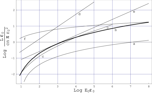
Figure 8: Plot of the quantity $q_{TPP}=L_{TPP}/\chi$ (TPP energy loss rate $L_{TPP}$ normalized to $\chi=cn\pi r_{0}^{2}$) versus $s_{\perp}=\varepsilon_{0}E_{0}$, compared with the analogous quantity $q_{ICS}=L_{ICS}/\chi$ concerning ICS energy loss rate $L_{ICS}$ (curve ($f$)). Curve ($b$) is obtained on the basis of precise calculations performed in this work. Curves ($c$), ($d$), ($e$) and ($a$) represent some approximations based on the results of Mastichiadis et al [4], Mastichiadis et al [2], Dermer and Schlickeiser [9] and Feenberg and Primakoff [10], respectively.

The normalized losses $q_{TPP}$ and $q_{ICS}$ versus $s_{\perp}$ are compared graphically in figure 8. There, curve ($f$) represents the dependence $q_{ICS}(s_{\perp})$ given by equation (2q). Curve ($b$) is obtained on the basis of precise numerical calculations performed in this work. It can be seen that, according to our results, TPP losses become prevalent and increase above ICS losses at values of $s_{\perp}$ exceeding a threshold $s_{th}\sim 10^{8}$. Certainly, this threshold is considerably higher (five orders of magnitude) than another threshold $s^{*}=250$ at which the interaction lengths of TPP and ICS become equal [4]. An estimate of $s_{th}$ derived from the equality $q_{TPP}(s_{\perp})=q_{ICS}(s_{\perp})$ (by using equations (2p) and(2q)) is $s_{th}\simeq 1.6\times 10^{8}$.

The estimate of $q_{TPP}(s_{\perp})=(5/\pi)\alpha_{f}s_{\perp}^{1/4}[\frac{28}{9}\ln(2s_{\perp})-\frac{218}{27}]$ obtained by Mastichiadis et al in 1991, is shown by curve ($c$). The threshold predicted in this case is $s_{th}\simeq 10^{6}$. Curve ($e$) represents the estimate $q_{TPP}(s_{\perp})=\frac{32}{9}\alpha_{f}s_{\perp}^{1/2}$obtained by Dermer and Schlickeiser [9]. It predicts a threshold $s_{th}\simeq 2\times 10^{5}$. Two more estimates of the dependence $q_{TPP}(s_{\perp})$ obtained from the results of [10] and [2] are illustrated by curves ($a$) and ($d$), and give unrealistically high and low thresholds, respectively. So, the consideration performed here, of the results obtained by different authors for the primary-electron energy loss rate due to TPP, confirms the existence of a tendency to a permanent improvement of the calculation accuracy. Because of the efforts to overcome the calculation difficulties and additionally increase the calculation precision, one can accept the results obtained here as reliable and accurate. They show that the electron energy losses due to TPP, e.g. in cascading processes occurring in pulsars ([3], [9], [13]) or in photon background field ([2], [4], [14]), are lower than those formerly predicted. The differences between the results for DDCS, SDCS, $E_{m}(E_{0},s),$and $E_{mi}(E_{0},s_{\perp})$ obtained here and those obtained in other works might lead to differences in the results from modelling electron-photon cascading in a soft photon field. Certainly, the detailed simulations now in progress will reveal the influence on the final results of the differences and factors discussed in this paper.

3 Conclusion

In order to develop a Monte Carlo code for three-dimensional modelling of TPP, we have undertaken a series of systematic precise calculations of DDCS and SDCS with respect to the produced electron and positron energies, as well as of the total cross-sections of TPP in the laboratory frame. The behaviour of the mean produced-particle energies has also been investigated in detail. To avoid crucial irregularities and sharp variations of the integrand, and extremely short integration intervals in the expressions of DDCS, SDCS, total cross-section, and mean produced-particle energy, we have used some appropriate mathematical approaches such as suitable changes of variables, optimum-power spline technique etc. These approaches lead to simpler and regular expressions of the cross-sections as well as to stable, accurate and accelerated calculation procedures. In addition, the use of the modern powerful program code Mathematica, working with arbitrary precision numbers, allowed us to obtain reliable high-precision results. Thus, the DDCS, SDCS and total cross-section have been computed for a variety of initial and final parameters characterizing TPP. The results for the total cross-section are in excellent agreement with ones obtained by other authors. However, there are some discrepancies in the results for DDCS and SDCS that might lead to differences in the results from modelling.

The mean produced-particle energy $E_{m}$ is analytically confirmed (in a general form) to be proportional to the incoming electron energy $E_{0}$ and to a function $f(s)$ of the collisional parameter $s$ only, i.e. $E_{m}=E_{m}(E_{0},s)=E_{0}f(s)$. It is also confirmed analytically that in an isotropic and monochromatic soft photon field the mean produced-particle energy $E_{mi}$ (averaged over the angle of collision $\theta$) is proportional to $E_{0}$ and a function $\varphi(s_{\perp})$ of the product $s_{\perp}=\varepsilon_{0}E_{0}$, i.e. $E_{mi}=E_{mi}(E_{0},s_{\perp})=E_{0}\varphi(s_{\perp})$. Such a general behaviour established of $\ E_{m}$ and $E_{mi}$ is in agreement with the results of other authors ([2], [4], [9], [10]). However, there are some essential differences that would also lead to different results from modelling. So, the mean produced-particle energy $E_{m}$ or $E_{mi}$ obtained here is proportional (apart from $E_{0}/s$ or $E_{0}/s_{\perp}$) to $\ln^{2}(2s)$ or $\ln^{2}(2s_{\perp})$, respectively (see equations (2i) and (2m)). At the same time, some earlier investigations of this question have led to a proportionality to a power function such as $s^{0.5}$ [9], $s_{\perp}^{0.44}$ [2] or $s_{\perp}^{0.25}$ [4]. The indicated differences in the determination of $E_{mi}$ lead to differences in the determination of that threshold level of $s_{\perp}=s_{th}$ above which the primary-electron energy losses due to TPP become prevalent over the ICS energy losses. It is shown here that the value of $s_{th}\sim 10^{8}$, that differs from the values of $s_{th}\sim 10^{6}$ [4] or $2\times 10^{5}$ [9] obtained formerly. The last-mentioned result means that there has been some overestimation of the role of TPP energy losses in some astrophysical studies ([2]-[4], [9], [13], [14]).

Appendix. Expression of the integrand function $X$.

The integrand function $X=X(E_{0},\varepsilon_{0},s,E_{+},E_{-},\xi,\eta,\phi_{+})$ is expressible in the following (possibly the only one) viewable and compact form that facilitates the programming and the calculations to be performed (see also [1], [15], [16]):

$$X=X_{U}+X_{V}+X_{W},$$

where

$$X_{U}=U+S_{1}U+S_{2}U+S_{3}U+S_{2}S_{1}U+S_{3}S_{1}U+S_{3}S_{2}U+S_{3}S_{2}S_{1}U,$$

$$X_{V}=V+S_{1}V+S_{2}V+S_{3}V+S_{2}S_{1}V+S_{3}S_{1}V+S_{3}S_{2}V+S_{3}S_{2}S_{1}V,$$

$$X_{W}=W+S_{1}W+S_{2}W+S_{3}W+S_{2}S_{1}W+S_{3}S_{1}W+S_{3}S_{2}W+S_{3}S_{2}S_{1}W;$$

$S_{1}$, $S_{2}$, and $S_{3}$ denote the substitution:

$$S_{1} = \overline{k}\leftrightarrow-\overline{k},\quad\ \overline{p_{0}}\leftrightarrow\overline{p_{r}},\quad\ \overline{p_{-}}\leftrightarrow-\overline{p_{+}},$$

$$S_{2} = \overline{p_{0}}\leftrightarrow-\overline{p_{+}},$$

$$S_{3} = \overline{p_{r}}\leftrightarrow\overline{p_{-}},$$

where (with respect to the laboratory frame) $\overline{k}=\{\overrightarrow{k},\varepsilon_{0}\}$ is the four-vector of the incoming photon; $\overline{p_{0}}=\{\overrightarrow{p_{0}},E_{0}\}$ is the four-vector of the incoming primary electron, and $\overline{p_{r}}=\{\overrightarrow{p_{r}},E_{r}\}$ is the four-vector of the recoiling primary electron; $\overline{p_{+}}=\{\overrightarrow{p_{+}},E_{+}\}$ and $\overline{p_{\_}}=\{\overrightarrow{p_{-}},E_{-}\}$ are the four-vectors of the produced positron and electron, respectively; $\overrightarrow{k_{0}}$, $\overrightarrow{p_{0}}$, $\overrightarrow{p_{r}}$, $\overrightarrow{p_{+}}$ and $\overrightarrow{p_{-}}$ are the corresponding three-component momentum vectors, and $\varepsilon_{0}$, $E_{0}$, $E_{r}$, $E_{+}$, and $E_{-}$ are the corresponding energy values. The module of each three-component vector $\overrightarrow{v}$ is denoted by $v$.

The expressions of $U$, $V$, and $W$ are:

$$U={\textstyle\frac{1}{2}}(1/(1+\tau_{1})^{2})\{(1/k_{3}^{2})[-k_{3}(k_{1}\tau_{2}+k_{0}\sigma_{3})+\tau_{1}k_{3}-\tau_{2}\sigma_{1}-\tau_{3}\sigma_{3}$$

$$\hbox to0.0pt{\hss${}+{}$}k_{1}\tau_{2}+k_{0}\sigma_{3}-k_{2}k_{3}+k_{2}+\tau_{1}+2k_{3}-\sigma_{2}+2]$$

$$\hbox to0.0pt{\hss${}+{}$}(1/(k_{2}k_{3}))[\sigma_{2}(k_{1}(\tau_{2}+\tau_{3})-\sigma_{1}\tau_{2}-\sigma_{3}\tau_{3})+k_{2}(\sigma_{1}\tau_{2}+\sigma_{3}\tau_{3}-2\tau_{3}\sigma_{1})$$

$$\hbox to0.0pt{\hss${}+{}$}\sigma_{2}(\tau_{1}-\sigma_{2}+2k_{2})-k_{0}k_{1}-\tau_{1}k_{2}+2\sigma_{2}-k_{2}]\},$$

$$V={\textstyle\frac{1}{4}}(1/((1+\tau_{1})(1-\sigma_{2})))\{(1/(k_{0}k_{3}))[2(k_{0}-k_{3}-2\tau_{3})+k_{0}(k_{1}+\tau_{1}+\sigma_{1}-\sigma_{2}+\sigma_{3})$$

$$\hbox to0.0pt{\hss${}+{}$}k_{3}(-k_{2}-\tau_{1}+\tau_{2}+\sigma_{2}-\sigma_{3})+\tau_{3}(-k_{1}-k_{2}+2\sigma_{2}-2\tau_{1})$$

$$\hbox to0.0pt{\hss${}+{}$}k_{0}(\sigma_{1}(-\sigma_{2}-\tau_{2})-2\sigma_{3}(k_{3}+\tau_{3}))+k_{3}(\tau_{1}\tau_{2}+\sigma_{1}\tau_{2}+2\sigma_{3}\tau_{3})$$

$$\hbox to0.0pt{\hss${}+{}$}\tau_{3}(2(\tau_{2}\sigma_{1}+\sigma_{3}\tau_{3})-k_{1}\tau_{2}+k_{2}\sigma_{1})]\}$$

$$\hbox to0.0pt{\hss${}-{}$}{\textstyle\frac{1}{4}}(1/((1+\tau_{1})(1-\sigma_{2})))\{(1/(k_{0}k_{2}))[2(k_{0}-k_{2}-2\tau_{2})$$

$$\hbox to0.0pt{\hss${}+{}$}k_{0}(k_{1}+\tau_{1}+\sigma_{3}-\sigma_{2}+\sigma_{1})+k_{2}(-k_{3}-\tau_{1}+\tau_{3}+\sigma_{2}-\sigma_{1})$$

$$\hbox to0.0pt{\hss${}+{}$}\tau_{2}(-k_{1}-k_{3}+2\sigma_{2}-2\tau_{1})+k_{0}(\sigma_{3}(-\sigma_{2}-\tau_{3})-2\sigma_{1}(k_{2}+\tau_{2}))$$

$$\hbox to0.0pt{\hss${}+{}$}k_{2}(\tau_{1}\tau_{3}+\sigma_{3}\tau_{3}+2\sigma_{1}\tau_{2})+\tau_{2}(2(\tau_{3}\sigma_{3}+\sigma_{1}\tau_{2})-k_{1}\tau_{3}+k_{3}\sigma_{3})]\},$$

$$W={\textstyle\frac{1}{8}}(1/((1+\tau_{1})(\sigma_{1}-1)))\{(2/k_{2}^{2})[2k_{1}k_{2}\tau_{3}+k_{2}(-k_{0}-k_{1}+k_{3}-\tau_{1}+\tau_{3}+\sigma_{1})$$

$$\hbox to0.0pt{\hss${}+{}$}2\tau_{3}(\sigma_{3}-k_{1})+k_{0}+k_{1}-2k_{2}-k_{3}-\tau_{1}-\tau_{2}+\tau_{3}+\sigma_{1}+\sigma_{2}-\sigma_{3}-2]$$

$$\hbox to0.0pt{\hss${}+{}$}(1/(k_{2}k_{0}))[2(\sigma_{3}(k_{2}\tau_{3}+k_{3}\tau_{2}-k_{0}(\sigma_{2}+\tau_{3})+2\tau_{2}\tau_{3})+\tau_{3}(k_{2}\tau_{1}-k_{1}\tau_{2}))$$

$$\hbox to0.0pt{\hss${}+{}$}2k_{0}(k_{1}-k_{3}+\tau_{1}+\tau_{2}-\tau_{3}-{\textstyle\frac{1}{2}}\sigma_{1}-\sigma_{2}+\sigma_{3})+k_{1}(2k_{3}-\tau_{3}+\sigma_{2})$$

$$\hbox to0.0pt{\hss${}+{}$}k_{2}(2\tau_{3}+\sigma_{1}-2\tau_{1}-2\tau_{2})+k_{3}(\tau_{1}-\sigma_{3})-2\tau_{2}(\tau_{1}+\tau_{2}-\tau_{3}-\sigma_{1}-\sigma_{2}+\sigma_{3})$$

$$\hbox to0.0pt{\hss${}+{}$}2(k_{1}-k_{3})+k_{0}-k_{2}-4\tau_{2}]$$

$$\hbox to0.0pt{\hss${}+{}$}(1/(k_{2}k_{3}))[2(\sigma_{3}(k_{3}\tau_{2}-k_{3}\tau_{3}-k_{2}\tau_{3}-k_{0}\sigma_{2}+2\sigma_{2}\tau_{3})+\tau_{3}(\sigma_{1}k_{2}-k_{1}\sigma_{2}))$$

$$\hbox to0.0pt{\hss${}+{}$}k_{0}(2k_{1}+2k_{3}-\sigma_{1}-\sigma_{3})+k_{1}(2k_{3}+\tau_{2}+\tau_{3})+k_{2}(\tau_{1}-2\tau_{3}-2\sigma_{1}-2\sigma_{2})$$

$$\hbox to0.0pt{\hss${}+{}$}k_{3}(\tau_{1}+2(\tau_{2}-\tau_{3}-\sigma_{1}-\sigma_{2}+\sigma_{3}))$$

$$\hbox to0.0pt{\hss${}+{}$}2\sigma_{2}(-\tau_{1}-\tau_{2}+\tau_{3}+\sigma_{1}+\sigma_{2}-\sigma_{3})+(-2k_{0}-2k_{1}+k_{2}+k_{3}-4\sigma_{2})]$$

$$\hbox to0.0pt{\hss${}+{}$}(1/(k_{0}k_{3}))[4\sigma_{3}(k_{3}+\tau_{3})(k_{0}-\tau_{3})+2\tau_{3}(\tau_{1}+\tau_{2}-\tau_{3}-\sigma_{1}-\sigma_{2}+\sigma_{3})$$

$$\hbox to0.0pt{\hss${}+{}$}k_{0}(-2\tau_{2}+2\tau_{3}-2k_{2}-3\sigma_{3})+k_{1}(2k_{2}-\tau_{2}+2\tau_{3}+\sigma_{2})$$

$$\hbox to0.0pt{\hss${}+{}$}k_{2}(2k_{3}+\tau_{1}+2\tau_{3}-\sigma_{1})+k_{3}(-2\tau_{3}-2\sigma_{2}+3\sigma_{3})$$

$$\hbox to0.0pt{\hss${}+{}$}2k_{1}-2k_{2}+3k_{3}-3k_{0}+4\tau_{3}]\}.$$

They are functions of the invariant products:

$$k_{0} = \overline{p_{0}}.\overline{k}=-s,\qquad\tau_{1}=\overline{p_{0}}.\overline{p_{r}}\,,\qquad\sigma_{1}=\overline{p_{+}}.\overline{p_{r}}\,,$$

$$k_{1} = \overline{p_{r}}\,.\overline{k},\qquad\qquad\;\tau_{2}=\overline{p_{0}}.\overline{p_{-}},\qquad\sigma_{2}=\overline{p_{+}}.\overline{p_{-}},$$

$$k_{2} = \overline{p_{-}}.\overline{k},\qquad\qquad\;\tau_{3}=\overline{p_{0}}.\overline{p_{+}},\qquad\sigma_{3}=\overline{p_{r}}.\overline{p_{-}},$$

$$k_{3} = \overline{p_{+}}.\overline{k},$$

which are connected, because of the energy-momentum conservation laws, by the relations:

$$\sigma_{3} = k_{0}+1-\sigma_{1}-\sigma_{2},$$

$$\sigma_{2} = k_{0}-k_{1}-\tau_{1},$$

$$\sigma_{1} = k_{0}-k_{2}-\tau_{2},$$

$$\tau_{1} = k_{0}-1-\tau_{3}-\tau_{2},$$

$$k_{1} = k_{0}-k_{3}-k_{2};$$

where

$$k_{0}=-E_{0}\varepsilon_{0}(1-\beta\cos\theta)=-s\qquad\mathrm{(section\ 2.1)},$$

$$k_{2}=p_{-}k[y\cos\theta_{k}+(1-y^{2})^{1/2}\cos\phi_{-}\sin\theta_{k}]-E_{-}\varepsilon_{0},$$

$$k_{3}=p_{+}k[x\cos\theta_{k}+(1-x^{2})^{1/2}\cos\phi_{+}\sin\theta_{k}]-E_{+}\varepsilon_{0},$$

$$\tau_{2}=p_{-}p_{0}[y\cos\theta_{0}-(1-y^{2})^{1/2}\cos\phi_{-}\sin\theta_{0}]-E_{-}E_{0},$$

$$\tau_{3}=p_{+}p_{0}[x\cos\theta_{0}-(1-x^{2})^{1/2}\cos\phi_{+}\sin\theta_{0}]-E_{+}E_{0},$$

$$\beta=p_{0}/E_{0},$$

$$\cos\theta_{0}=\cos\theta\cos\theta_{k}+\sin\theta\sin\theta_{k},$$

$$\sin\theta_{0}=\sin\theta\cos\theta_{k}-\cos\theta\sin\theta_{k},$$

$$\sin\theta_{k}=(1-\cos^{2}\theta_{k})^{1/2},$$

$$\cos\theta_{k}=(k+p_{0}\cos\theta)/P_{tot},$$

$$\phi_{-}=\phi_{+}-\alpha,$$

$$\alpha=[(1+s-E_{tot}(E_{+}+E_{-})+E_{+}E_{-}+P_{tot}(p_{+}x+p_{-}y)$$

$$\hbox to0.0pt{\hss${}-{}$}p_{+}p_{-}xy)/(p_{+}p_{-}(1-x^{2})^{1/2}(1-y^{2})^{1/2})],$$

$$P_{tot}=(p_{0}^{2}+k^{2}+2p_{0}k\cos\theta)^{1/2},$$

$$p_{k}=\varepsilon_{0},\quad p_{0}=(E_{0}^{2}-1)^{1/2},$$

$$p_{-}=(E_{-}^{2}-1)^{1/2},\quad p_{+}=(E_{+}^{2}-1)^{1/2}.$$

With $\theta_{0}$ and $\theta_{k}$ we have, respectively, denoted the polar angles of the incoming electron and photon momenta with respect to the axis along $\overrightarrow{P_{tot}}=\overrightarrow{p_{0}}+\overrightarrow{k}$. In this case $\theta_{0}+\theta_{k}=\theta$, where $\theta$ is the angle between $\overrightarrow{p_{0}}$ and $\overrightarrow{k}$, i.e. the angle of collision. The azimuthal angles of the produced electron and positron are $\phi_{-}$ and $\phi_{+}$, respectively . They are accounted for in such a way that $\phi_{k}=0$ and $\phi_{0}=\pi$, where $\phi_{k}$ and $\phi_{0}$ are the azimuthal angles of the incoming photon and electron, respectively [2].

The variables $\xi$ and $\eta$ are introduced by the substitutions (section 2.1, equations (2a) and (2b)):

$$x = x(\xi)=\xi/l+x_{\min}\quad(l>1),$$

$$y = y(\xi,\eta)=[y_{\max}(x)+y_{\min}(x)\eta^{2}]/(1+\eta^{2}).$$

The remaining designations are given in section 2.1.

References

References

- [1] Mork K J 1971 Phys. Nor. 6 51
- [2] Mastichiadis A, Marscher A P and Brecher K 1986 Astrophys. J. 300 178
- [3] Mastichiadis A, Brecher K and Marsher A P 1987 Astrophys. J. 314 88
- [4] Mastichiadis A 1991 Mon. Not. R. Astron. Soc. 253 235
- [5] Mastichiadis A, Protheroe R J and Szabo A P 1994 Mon. Not. R. Astron. Soc. 266 910
- [6] Anguelov V, Petrov S and Vankov H 1995 Papers of 24th ICRC (Roma) pp 790-3
- [7] Wolfram S 1996 Mathematica (Cambridge: Cambridge University Press)
- [8] Haug E 1981 Z.Naturforsch. 36 413
- [9] Dermer C D and Schlickeiser R 1991 Astron.Astrophys. 252 414
- [10] Feenberg E and Primakoff H 1948 Phys. Rev. 73 449
- [11] Blumenthal G R 1971 Phys. Rev. D 3 2308
- [12] Blumenthal G R and Gould R J 1970 Rev. Mod. Phys. 42 237
- [13] Sturner S J 1995 Astrophys. J. 446 292
- [14] Lee S 1998 Phys. Rev. D 58 043004
- [15] Jarp S and Mork K J 1973 Phys. Rev. D 8 159
- [16] Motz J W, Olsen H A and Koch H W 1969 Rev. Mod. Phys. 41 581