A search for precursors of Ultracompact Hii Regions in a sample of luminous IRAS sources.

Abstract

The James Clerk Maxwell Telescope has been used to obtain submillimeter and millimeter continuum photometry of a sample of 30 IRAS sources previously studied in molecular lines and centimeter radio continuum. All the sources have IRAS colours typical of very young stellar objects (YSOs) and are associated with dense gas. In spite of their high luminosities (L$\;\lower 2.58334pt\hbox{$\sim$}\kern-7.75pt\raise 2.79857pt\hbox{$>$}\;10^{4}$ $L_{\odot}$), only ten of these sources are also associated with a radio counterpart. In 17 cases we could identify a clear peak of millimeter emission associated with the IRAS source, while in 9 sources the millimeter emission was either extended or faint and a clear peak could not be identified; upper limits were found in 4 cases only.

The submm/mm observations allow us to make a more accurate estimate of the source luminosities, typically of the order of 10⁴ $L_{\odot}$. Using simple greybody fitting model to the observed spectral energy distribution, we derive global properties of the circumstellar dust associated with the detected sources. We find that the dust temperature varies from 24 K to 45 K, while the exponent of the dust emissivity $vs$ frequency power-law spans a range 1.56$<\beta<$2.38, characteristic of silicate dust; total circumstellar masses range up to more than 500 $M_{\odot}$.

We present a detailed analysis of the sources associated with millimeter peaks, but without radio emission. In particular, we find that for sources with comparable luminosities, the total column densities derived from the dust masses do not distinguish between sources with and without radio counterpart. We interpret this result as an indication that dust does not play a dominant role in inhibiting the formation of the Hii region. We examine several scenarios for their origin in terms of newborn ZAMS stars and although most of these (e.g. optically thick Hii regions, dust extinction of Lyman photons, clusters instead of single sources) fail to explain the observations, we cannot exclude that these sources are young stars already on the ZAMS with modest residual accretion that quenches the expansion of the Hii region, thus explaining the lack of radio emission in these bright sources. Finally, we consider the possibility that the IRAS sources are high-mass pre-ZAMS (or pre-H-burning) objects deriving most of the emitted luminosity from accretion.

1 Introduction

The last few years have seen a rapidly growing observational activity aimed at the identification of intermediate- and high-mass star forming sites exhibiting a wide range of evolutionary stages from UltraCompact Hii  (UC Hii) regions (Wood & Churchwell [1989]), to “Hot Cores” (Cesaroni et al. [1994]), and proto-Ae/Be stars (Hunter et al. [1998]; Molinari et al. [1998b]). The characterization of the earliest stages of high-mass star formation, given their shorter evolutionary timescales, is more difficult than for low-mass objects. The observational approach to the search of the youngest high-mass forming objects was first formulated by Habing & Israel ([1979]): the likely candidates must have high luminosity, be embedded in dense circumstellar environments, and they should not be associated with Hii regions.

We have undertaken a systematic study aimed at the identification of a sample of massive protostellar candidates; the whole process is summarized in Fig. 1. Initially, a list of 260 sources with 60$\mu$m flux greater than 100 Jy was compiled from the IRAS-PSC2, according to the colour criteria of Richards et al. ([1987]) for compact molecular clouds. This sample was then divided into two groups according to their [25$-$12] and [60$-$12] colours: the High sources, which have [25$-$12]$\geq$0.57 and [60$-$12]$\geq$1.3 characteristic of association with UC Hii regions (Wood & Churchwell [1989]), and the Low sources, with [25$-$12]$<$0.57 or [60$-$12]$\leq$1.3. We note that the [25$-$12] and [60$-$12] IRAS colours of Low sources are different also from those of T Tau or Herbig Ae/Be stars, but are similar to those of normal Hii regions (Palla et al. [1991]). The lower H₂O maser detection rate found towards Low sources (a factor of 3 lower than for High sources) was interpreted as an indication of relative youth, and we concluded that the Low group might contain a fraction of young sources whose formation process has not yet proceeded far enough to produce a fully-developed ZAMS star (Palla et al. [1991]); the Low group thus represents an optimum target group to search for high-mass protostars.

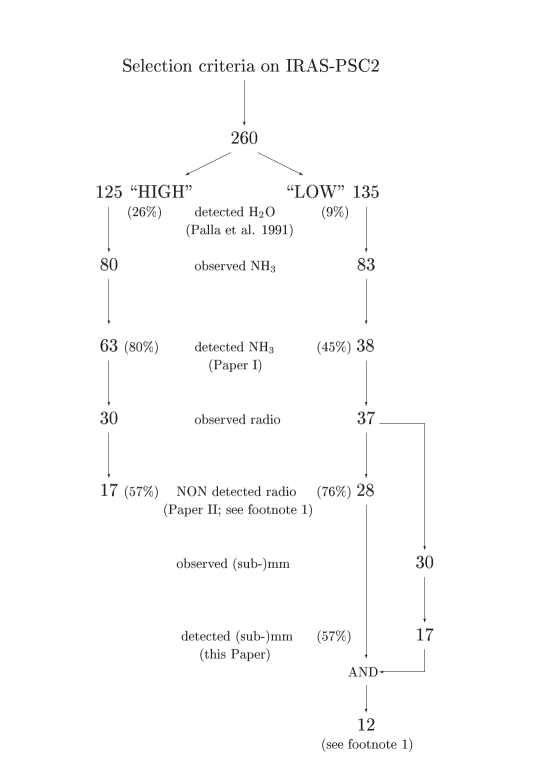
Figure 1: Flow-chart for the selection of the sample of intermediate-to-high mass candidate protostellar objects. The final sample consists of 12 objects detected in the (sub-)mm and not associated with radio continuum. However, one of these objects (#12 in Table 2) has been recently detected at 3.6 cm, as explained in footnote 1.)

We observed the NH₃(1,1) and (2,2) lines in a subsample of 80 High and 83 Low sources to check for association with dense gas (Molinari et al. [1996], hereafter Paper I). A result was that the linewidth ratio $\Delta v_{22}/\Delta v_{11}$ is correlated with the [25$-$12] colour, increasing from values  $\sim$$<$ 1 to values  $\sim$$>$ 1 going from Low to High sources. We speculated that lower linewidth ratios in Low sources were indicative of a lesser degree of activity in the central regions with respect to the High sources. A critical test to our conjecture was to verify the occurrence of radio continuum emission from High and Low sources. Molinari et al. ([1998a], hereafter Paper II) observed with the VLA at 2 and 6-cm, 37 Low and 30 High  sources with ammonia detections. We found that 76% of Low and 57% of High sources are not associated with UC Hii regions , confirming the goodness of the FIR colour-based separation between High and Low as an indicator of presence/absence of a compact radio counterpart, and further reinforcing our assumption about the relative youth of the Low group; this idea is also supported by the recent identification (Molinari et al. [1998b]) of a massive Class 0 (André et al. [1993]) object in the Low group.

The purpose of the present observations is twofold. On the one hand we wish to complete the selection process started by Palla et al. ([1991]) by identifying those objects of the initial sample which are associated with peaks of dense gas and dust and do not show a radio continuum counterpart (see Fig. 1 and Sect. 3.1). On the other hand, in order to verify that different evolutionary stages are present in the Low group, we need to understand the physical nature of the distinction between Low sources with and without radio counterpart: is the Hii region really absent in the latter group, or is some mechanism, independent of the evolutionary state of the sources, responsible for inhibiting the formation of the Hii region ? It is a general result from radio continuum observations of UC Hii regions (e.g. Wood & Churchwell [1989]; Paper II) that the Lyman continuum flux required to explain the observed radio continuum emission is generally lower than what is expected based on the luminosity and spectral type of the ionizing star. Dust certainly plays a role by absorbing a relevant fraction of the ionizing UV continuum (Aannestad [1989]) and one may ask whether the high rate of non detection in radio continuum for the Low sources might not be accounted for by the properties of the dust in their circumstellar environment. Millimeter continuum observations are therefore mandatory to shed light on this issue. So far, the only information regarding the association of the Low sources with dense circumstellar environments comes from the single-pointing ammonia measurements (Paper I) and it is important to check for the presence of dense and compact cores. The present paper describes such observations; details of the observations and data reduction procedures can be found in Sect. 2, while data analysis methods and results are described in Sect. 3. The derived global properties and the nature of the detected sources are discussed in Sect. 4 and 5; the main conclusions are summarized in Sect. 6.

2 Observations

Observations were performed with the James Clerk Maxwell Telescope (JCMT) from 3 to 5 September 1994, and the UKSERV program provided service observations on several occasions between November 1994 and June 1995. We observed 30 Low sources, 10 of which are associated with radio continuum (Paper II, but see footnote 1). In each observing session the common user UKT14 bolometer (Duncan et al. [1990]) was used, with a focal plane aperture of 65 mm at all wavelengths; this corresponds to a $\sim 18$^′′.5 HPBW for wavelengths from 0.35 to 1.1 mm, increasing to 19^′′.5 and 27^′′at 1.3 and 2.0 mm respectively (Sandell [1994]). Azimuthal chopping was done with an amplitude of 60^′′, and frequency of 7.813 Hz.

Observations were centered on the IRAS PSC-2 coordinates and one or more cross maps in [Az, El] at 1.1 mm with 10^′′ spacing (called a FIVEPOINTS cycle) were done to maximize the signal and locate the position of the millimeter emission peak, where subsequently observations in the other bands were made. The control computer automatically estimated the centroid position from each FIVEPOINTS cycle; if this position was more distant than 3-4^′′ from the center of the cross map, another FIVEPOINTS cycle centered on this new position was performed. Obviously no photometry was done when no 1.1 mm emission was detected during the maximization procedure, or when the emission was faint and diffuse and an emission peak could not identified. During the September 1994 run only 0.8–2.0 mm photometry could be done as weather conditions prohibited observations at shorter wavelengths. In these cases UKSERV provided the needed photometry, pointing at the previously determined 1.1 mm peak and performing FIVEPOINTS cycles at 0.45 mm to estimate possible shifts between emission centroids at different wavelengths. UKSERV also provided complete 0.35–2.0 mm photometry of the few sources which had not been observed in the September 1994 run.

Table 1: Journal of Observations

Date/code	$\overline{\tau_{CSO}}$	Band	$\tau$	Gain	Int.
dd-mm-yy		(mm)		(Jy/mV)	unc.
03-09-94/A	0.28	0.8	1.42	17.31	6%
		1.1	0.58	12.82	3%
		1.3	0.48	12.70	2%
		2.0	0.23	36.98	1%
04-09-94/B	0.22	0.8	1.67	12.07	11%	1
		1.1	0.66	11.87	5%	1
		1.3	0.54	11.74	3%	1
		2.0	0.29	34.25	2%	1
05-09-94/C	0.15	0.8	1.16	10.61	5%
		1.1	0.39	12.23	3%
		1.3	0.19	14.52	2%
		2.0	0.26	31.32	1%
30-11-94/S-D	0.02	0.45	$-$	24.09	10%	2
		0.8	$-$	8.12	5%	2
		1.3	$-$	10.98	15%	2
19-01-95/S-E	$-$	0.35	1.09	19.70	11%
		0.45	1.02	14.64	9%
20-01-95/S-F	$-$	0.35	$-$	57.74	10%	3
		0.45	$-$	35.82	10%	3
		0.8	$-$	9.43	5%	3
		1.1	$-$	10.69	4%	3
		1.3	$-$	14.13	15%	3
		2.0	$-$	37.07	6%	3
06-06-95/S-G	$-$	0.35	0.77	65.37	5%
		0.45	1.02	19.12	9%

Notes to Table:

1 - Airmass coverage of the standards was not sufficient to determine reliable optical depths and gains. So, standards done in this night were merged with the same standards done in the previous night, as the signal from the same standards at same airmass in the two nights is comparable within few %.

2 - Only 1 source and 1 standard were observed in this night.

3 - Airmass coverage of the observed standards was not sufficient to determine optical depths and gains from Eq. (1). Each observed source was reduced using a standard observed immediately before or after and at comparable (within 0.1) airmasses.

Standard sources from the compilation of Sandell ([1994]) were observed at different airmasses to allow an estimate of the optical depths $\tau_{\lambda}$ and detector gains $G_{\lambda}$ (in Jy/mV) in the various bands. Following Stevens & Robson ([1994]), the flux $F_{\lambda}$ (in Jy) and the signal $S_{\lambda}$ (as measured in mV from the detector) of a source at a given airmass A can be expressed as

$$\ln~{}F~{}-~{}\ln~{}S~{}=~{}\ln~{}G_{\lambda}~{}+~{}\tau_{\lambda}~{}A.$$ (1)

We thus have a set of values [$\ln~{}F-\ln~{}S$, $A$] for each standard (where $S$ and $A$ come from the observations, and $F$ is tabulated by Sandell [1994]); a linear regression using all standards observed in the course of a night will then provide the $\tau_{\lambda}$ (the slope) and $G_{\lambda}$ (e-base power of the intercept). These values are then used to compute the standards’ fluxes which are compared to the tabulated values (Sandell  [1994]) to get an estimate of the standards’ intercalibration uncertainties in all bands: these are added in quadrature with the intrinsic statistical uncertainties of the measurements to get the total uncertainty.

Information about the observations is summarized in Table 1 where we give: [Column 1] date of observations and a code used to identify the session, where ‘S’ stands for ‘service observations’; [Column 2] the 1.3 mm optical depth as measured through continuous skydips by the nearby Caltech Submillimeter Observatory (CSO); [Column 3] the central wavelength of the photometric band; [Columns 4-5] optical depth and detector gain in each band; [Column 6] intercalibration uncertainty; [Column 7] notes.

If the airmass coverage of the standards was not sufficient to derive reliable optical depths and gains using Eq. (1)(sessions B and S-F), or if just one standard was observed (session S-D), each source was reduced using a standard at comparable airmass and observed immediately before or after the source; in this case only the gain is reported in Table 1, and the intercalibration uncertainty was conservatively assumed to be equal to the maximum, for each band, of the uncertainties estimated for all the other nights.

Using information in Table 1 we can compute fluxes of target sources in all bands. Four sources (#45, 75, 82 and 98) were mapped on-the-fly at 1.1 mm by chopping in an adjacent field with the telescope stepping by 4^′′ and integrating 2 seconds on each point; the final maps were reconstructed using the NOD2 software, and cover a 2^′$\times$ 2^′ field approximately. For other sources, limited information about the spatial distribution of the emission can be derived from the FIVEPOINTS cycles done to locate the emission peak. All the maps are presented in Fig. 2.

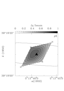
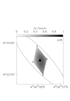
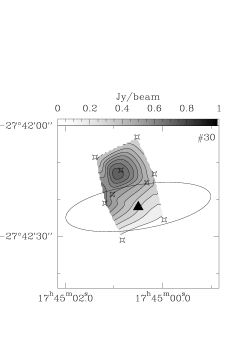
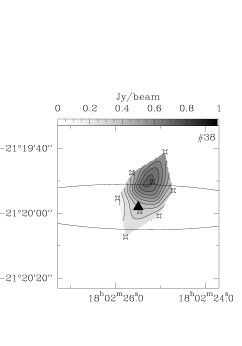
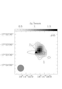
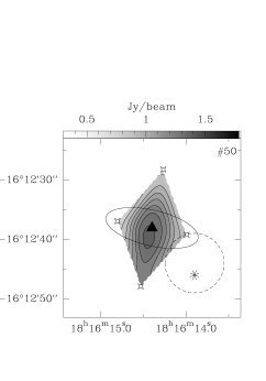
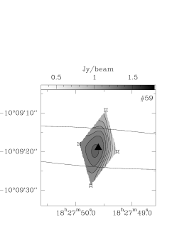
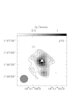
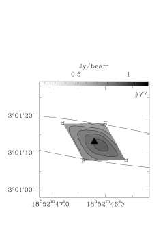
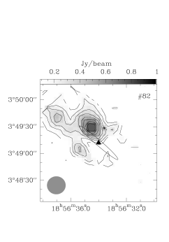
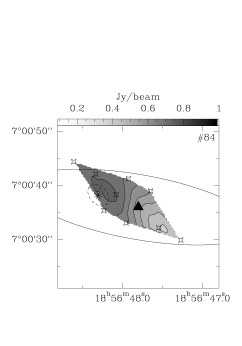
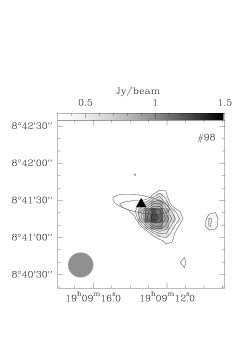
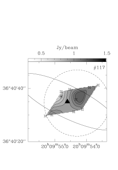
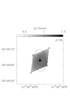
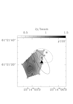
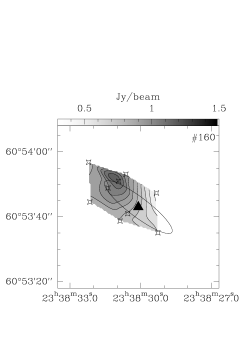
Figure 2: Maps of the $\lambda=1.1$mm emission for the Low sources where a clear emission peak was found. Most of them are reconstructed from the FIVEPOINTS crosses made to maximize the source signal and locate the peak. On-the-fly maps are presented for sources #45, 75, 82 and 98 (the grey circle on the bottom left indicates the telescope beam FWHM); note that the reconstruction of the maps with the NOD2 package was only possible at the telescope. It was not possible to make a very careful removal of mapping artifacts, and features other than the main peak are to be considered uncertain. The full triangles represent the nominal position of the IRAS source; the associated 1$\sigma$ error ellipse is also indicated with a full line. The small empty star-like symbols represent the observed positions during the FIVEPOINTS cycles. The positions and extensions (when resolved) of the associated radio counterparts are indicated as asterisks and dashed ellipses respectively. Contours levels are spaced at 10% of the maximum flux, and a greyscale is also superimposed for clarity. 16 out of 17 maps are shown because no FIVEPOINTS cycles for source #12 was done; new unpublished SCUBA maps show that the IRAS position for #12, used for the pointing in the present observations, coincides with a millimeter continuum peak.

3 Results and data analysis

Table 2: Observations

(1)	(2)	(3)	(4)	(5)	(7)	(7)	(8)	(9)	(10)	(11)
Mol #♣	Obs. code	IRAS Pos.		$\Delta_{1.1mmPos.}$	Observed Fluxes (Jy)
		$\alpha$(1950)	$\delta$(1950)		0.35	0.45	0.8	1.1	1.3	2.0
Detected Sources
8	S-F	05:13:45.8	+39:19:09.7	0,0	17(2)	7.0(0.7)	1.05(0.02)	0.38(0.02)	0.29(0.06)	0.09(0.05)
(12)a	S-F	05:37:21.3	+23:49:22.0	0b, 0b	41(5)	18(2)	2.73(0.03)	0.91(0.04)	0.7(0.1)	0.3(0.1)
28	S-F	06:58:27.9	$-$08:52:11.0	0, 0	5(1)	2.2(0.4)	0.36(0.03)	0.120(0.03)	0.13(0.05)	0.16(0.08)
30	S-E/Bc	17:45:00.5	$-$27:42:22.0	+6, +10	27(3)	15(2)	1.2(0.3)	0.40(0.07)	0.21(0.08)	$<$0.06
38	S-E/Bc,d	18:02:25.5	$-$21:19:58.0	$-$3, +8	80(9)	41(4)	3.9(0.5)	1.27(0.08)	0.89(0.04)	0.24(0.06)
45	S-E/Bc	18:14:29.8	$-$17:23:23.0	$-$9, +4	120(10)	60(5)	4.0(0.5)	1.63(0.09)	1.20(0.04)	0.29(0.06)
50	B	18:16:14.4	$-$16:12:38.1	0, 0	24(3)	14(1)	1.9(0.3)	0.44(0.04)	0.29(0.03)	0.16(0.08)
59	S-E/Cc	18:27:49.6	$-$10:09:19.0	0, 0	18.6(0.2)	9.3(0.9)	1.5(0.1)	0.33(0.03)	0.33(0.03)	0.18(0.04)
75	S-G/A	18:51:06.4	+01:46:40.0	0, 0	43(5)	24(2)	3.4(0.3)	1.16(0.05)	0.75(0.05)	0.14(0.08)
77	S-G/A	18:52:46.2	+03:01:13.0	$-$2, $-$2	26(2)	12(1)	1.5(0.2)	0.56(0.04)	0.39(0.04)	0.20(0.06)
82	S-G/C	18:56:34.0	+03:49:12.1	+8, +18	43(3)	23(2)	2.8(0.2)	0.87(0.03)	0.52(0.05)	0.18(0.08)
84	S-G/B	18:56:47.8	+07:00:36.1	+6, +3	18(1)	8.0(0.8)	1.2(0.2)	0.45(0.04)	0.32(0.02)	$<$0.4
98	S-G/B	19:09:13.4	+08:41:27.1	$-$10, $-$10	68(4)	32(3)	5.8(0.7)	1.6(0.1)	1.09(0.06)	0.4(0.1)
117	A	20:09:54.6	+36:40:35.1	$-$5, +2			0.9(0.2)	0.25(0.04)	0.20(0.04)	$<$0.4
136	B	21:30:47.3	+50:49:03.1	0, 0			2.1(0.3)	0.46(0.05)	0.37(0.07)	$<$0.4
155	B	23:14:01.9	+61:21:22.0	+9, $-$5			1.7(0.2)	0.31(0.06)	0.20(0.04)	0.11(0.06)
160	C	23:38:30.1	+60:53:43.0	+8, +8			2.6(0.2)	0.84(0.05)	0.52(0.03)	0.20(0.07)
Faint sources or sources without clear peak
36	B	18:01:25.1	$-$24:29:00.0					0.15(0.04)
57	A	18:25:37.8	$-$07:42:19.9					0.13(0.03)
68	A	18:39:39.8	$-$04:31:34.9					0.15(0.03)
87	A	18:58:38.1	+01:06:57.0					0.06(0.04)
122	A	20:21:43.3	+39:47:39.0					0.15(0.03)
125	A	20:27:51.0	+35:21:33.0					0.13(0.05)
129	A	20:33:21.3	+41:02:53.1					0.36(0.03)
Undetected Sources
66	A	18:36:23.1	$-$05:54:58.9					$<$0.1
70	A	18:42:25.5	$-$03:29:59.1					$<$0.1
86	A	18:57:10.6	+03:49:22.0					$<$0.2
91	A	19:01:15.5	+05:05:19.0					$<$0.2
Missed Primary Peak
(3)a	S-D	00:42:05.4	+55:30:54.1	+8, $-$4		0.6(0.5)	0.16(0.02)	0.017(0.007)
118	A	20:10:38.0	+35:45:42.0				1.0(0.2)	0.25(0.05)	0.12(0.04)	$<$0.3

^♣ underlined and bold-face indicates association with radio continuum emission (Paper II).

^asee footnote 1.

^bno FIVEPOINTS cycle done; however, we have SCUBA maps (unpublished) confirming that the pointed position is centered on a mm core.

^cfirst code refers to 0.35-0.45mm photometry.

^d0.45mm peak is 12^′′E, 2^′′S of 1.1mm peak.

The results of the observations are listed in Table 2, organized as follows; [Column 1] source number as in Paper I; [Column 2] code referring to the observing night (see Table 1); [Columns 3-4] source coordinates from the IRAS PSC-2; [Columns 5] ($\Delta\alpha$(^′′), $\Delta\delta$(^′′)) offset of 1.1 mm peak from IRAS position of the 1.1 mm emission peak to the IRAS coordinates; [Columns 6-11] fluxes (in Jy) observed at the given bands, with errors (in Jy) in parentheses (including both statistical and calibration uncertainties); upper limits are given at the 3$\sigma$ level.

Figure 3: The spectral energy distribution of the 17 detected Low sources (see Sect. 3) are reported below as plots of Flux density (Jy) against wavelength ($\mu$m). IRAS photometric points are represented by squares; triangles represent radio 2 and 6 cm fluxes when a radio counterpart is present. Submillimeter photometry, after removal of free-free contribution (see footnote 2), is indicated with asterisks. The solid lines represent model fit to the data as described in Sect. 3.2; the corresponding parameters are listed in Table 4. The SED for #12 does not report the recently detected 3.6 cm emission.

Inspecting the spectral energy distributions plotted in Fig. 3, one notes that in most cases the point at 2.0 mm, and sometimes also the point at 1.3 mm, lie above the fitted curve (compare also with the fits obtained as described in Sect. 3.2); we believe this is due to the different beamsizes of the UKT14 instrument at different wavelengths (see Sect. 2). The ratios between areas of the beam at the different wavelengths are A_1.3/A_(0.35-1.1)=1.1 and A_2.0/A_(0.35-1.1)=2.1; this means that in case of a source uniformly filling the 2.0 mm beam (27^′′), the measured 2.0 mm flux will be about a factor of 2 higher than what an extrapolation from lower wavelengths might suggest. Scaling 1.3 and 2.0 mm photometry by these factors is in most cases sufficient to bring those points to agree within the errorbars with the trend suggested by the 0.35–1.1 mm fluxes. A proper scaling of the fluxes would require knowledge of the (unknown) spatial brightness distribution.

The luminosities of our sources as listed in Paper I are based on the 4 IRAS-PSC2 fluxes, plus a correction to take into account emission longward of 100$\mu$m (Cohen [1973]); this correction is likely to overestimate the true luminosity, because it is assumed that the SED falls off as a black body. With the help of the new millimeter and submillimeter photometry we can derive a more accurate value for the luminosity of the observed sources.

With respect to Paper I, the distances have also been slightly revised for some sources. In Paper I all distances were estimated from the V_LSR of the (1,1) ammonia line, using the observed velocity field as determined by Brand & Blitz ([1993]); however, as noted by Brand & Blitz, the data are quite sparse for distances greater than 5 kpc from the Sun in the II^nd and III^rd galactic quadrant. In these cases one ought to estimate distances by using the analytical expression for the galactic rotation curve, rather than the observed velocity field; distances (and luminosities) for the affected sources have been updated accordingly.

3.1 Association of IRAS Low sources with millimeter counterparts

10 out of the 30 observed Low sources are associated with radio continuum emission (Paper II, but see footnote 1). We consider a source associated with a millimeter continuum counterpart, and hence a detection, only when a peak of emission is clearly detected. In 17 of the 30 observed sources we detected peaked millimeter emission. In 7 (out of 30) cases only faint millimeter emission was detected, or no clear peak was found; in 4 (out of 30) cases only upper limits could be established. In two cases (sources #3 and #118) only a relative maximum of millimeter emission was located by the automatic maximization procedure; these sources will be conservatively considered as non-detections. These numbers are summarized in Table 3, where we also give information about association with radio counterpart (Paper II) and H₂O masers (Palla et al. [1991]).

The overall millimeter detection rate is 17/30$\sim$57%; the mm detection rate does not distinguish between Low sources with (6/10=60%) and without (11/20=55%) a radio counterpart. Almost all (9/10) sources with H₂O masers are associated with a mm peak, while none of the sources with a maser has a radio counterpart. Because the occurrence of water masers generally preceeds the development of an UC Hii region (Churchwell et al. [1990]), this result, together with the 57% overall detection rate, is an independent confirmation of the validity of our approach to select massive protostars (see Fig. 1).

In the group of Low sources, we find young and old objects (see Sect. 1 and Paper II), i.e. both UC Hii and older, extended Hii regions. This way three out of four Low sources with a radio counterpart that are not associated with a mm-peak can be accounted for: in these sources the associated Hii regions are more extended ($<$2, 225, 2500 and 3600^′′2 for sources #3 (see footnote 1), 68, 91 and 129 respectively) than in 5 of the 6 Low sources with both an Hii region and a peak in the mm-emission ($<$2, 100, 3.8, 3.7, and 150^′′2 for sources # 12 (see footnote 1), 50, 82, 84, and 155S respectively). Only # 117 has relatively extended radio emission (625^′′2) and associated mm-emission. The lack of millimeter detection correlates with the extension of the Hii region and identifies the oldest sources of the sample. For the Low sources without a mm counterpart, the ammonia column density never exceeds 8$\times 10^{13}$ cm^-2 (Paper I), while it ranges between 10¹³ and 10¹⁵ cm^-2 in the Low sources detected in the millimeter. Hence one possible explanation for the non-detections in the millimeter is that the peak of emission is significantly displaced with respect to the nominal IRAS position, and our ammonia observations only detected the relatively lower-density peripheral regions of the core. Typically, at least two or three FIVEPOINTS crosses (see Sect. 2) were performed around the IRAS position, so that we could pick up the millimeter peak only if it was within $\sim$20^′′ from that position. Alternatively, the sources are not necessarily compact; the IRAS resolution at 100 $\mu$m is  $\sim$$>$  3^′, and the bulk of the FIR flux might arise from a relatively diffuse source. In this case either the column density is too low for millimeter detection, or we might have been chopping with both the ON and OFF beams in the diffuse source.

Table 3: Detection Summary

mm	Radio	Lowa	H2O maserb
Y	N	11	8
Y	Y	6	0
N	N	9	1
N	Y	4	0

^a radio detections include the two recent detections (see footnote 1).

^b based on Palla et al. ([1991])

3.2 Dust physical parameters

It is common practice to use submillimeter and millimeter radiation to trace the global properties of the dust. The assumption is that dust is optically thin at submillimeter and millimeter wavelengths up to column densities $N_{\rm H}\sim 10^{25}$ cm^-2 (Mezger  [1994]). In the usual formalism (Hildebrand [1983]), the emission is assumed to come from dust at a single temperature and density. The flux observed at each frequency can be expressed as:

$$F_{\nu}~{}=~{}{{M_{\rm D}}\over{d^{2}}}~{}\kappa_{\nu}~{}B(\nu,T)$$ (2)

where $M_{\rm D}$ is the dust mass, $d$ the distance, $\kappa_{\nu}$ the dust mass opacity parametrized as $\kappa_{\nu}=\kappa_{\nu_{0}}(\nu/\nu_{0})^{\beta}$, and $B(\nu,T)$ the Planck function. The temperature enters only in the Planck function and determines the wavelength of the peak of the continuum emission. The mass affects the overall level of continuum, while the opacity fixes both the absolute level and the slope of the submm continuum. The largest uncertainty in the mass determination comes from the assumption on the dust mass opacity. Hildebrand ([1983]) proposed a total gas+dust mass opacity of 0.1 cm² g^-1 at 250 $\mu$m, and in spite of the order-of-magnitude uncertainties that are generally believed to affect the $\kappa_{250}$ value, Ossenkopf & Henning ([1994]) concluded that a variation at most of a factor 5 can be expected depending on the presence of ice mantles on grains. To estimate the dust mass, temperature and emissivity law, we fit Eq.(2) to the available data points by minimising the $\chi^{2}$. For sources associated with radio counterpart we extrapolated the observed 2 and 6 cm radio continuum (Paper II) and subtracted this contribution from the observed millimeter fluxes before doing the fit. Twenty-five iterations were performed in which the search radius for minimum $\chi^{2}$ in each variable was decreased by a factor 1.25 each time a minimum of $\chi^{2}$ was reached. Reduced $\chi^{2}$ values at the end of the procedure were typically less than 3-4. We checked the repeatability of our results by running the fitting procedure with starting values for mass, temperature and dust opacity spanning one order of magnitude; the maximum variation in the final best fit values was of less than 2%, with the $\chi^{2}$ remaining constant to the second decimal digit. We also checked the sensitivity of the final $\chi^{2}$ as a function of the fit parameters, and we found that keeping the temperature fixed to a value within 10% of the best fit value yielded a $\chi^{2}$ higher by 80%, causing the fit to converge at mass and $\beta$ values different by respectively $\sim$30% and $\sim$10% from the best fit values. The repeatability and the high sensitivity of the $\chi^{2}$ to the fit parameters, suggests that the internal accuracy of the method is within a few percent.

The fitted spectral energy distributions are presented in Fig. 3. The peak of the continuum distribution is around 100 $\mu$m so the submm data only cannot guarantee a meaningful convergence of the fit. Therefore, we have also included the IRAS 60 and 100 $\mu$m fluxes and for each source computed, based on the fitted opacity and assuming an emitting area equal to the JCMT beamsize, the wavelength where the optical depth becomes greater than unity (in most cases $\lambda<$60 $\mu$m). Having estimated the mass, we can then derive the H₂ column density, assuming a gas/dust ratio of 100 by weight and a size of the emitting area equal to the beam size. The results of our analysis for the 17 sources with a millimeter peak are summarized in Table 4 organized as follows: [Column 1] source running number as in Papers I and II; [Columns 2-3] distance to the source in kpc and bolometric luminosity corrected as explained at the end of Sect. 3; [Column 4] $\beta$ value; [Column 5] total (gas+dust) mass; [Column 6] derived H₂ column density; [Column 7] dust temperature; [Column 8] wavelength where $\tau$=1.

Table 4: Derived Physical Parameters

#†	d	L	$\beta$	Mtot	N(H2)	Td	$\lambda_{\tau=1}$
	(kpc)	($L_{\odot}$)		($M_{\odot}$)	($10^{22}$cm-2)	(K)	($\mu$m )
8	10.80	39300	1.56	210	1.7	37	12
(12)a	1.17	470	1.62	8.8	5.9	27	29
28	4.48	5670	1.57	9.8	0.4	45	5
30	2.00	3500	1.98	17.6	4.1	35	37
38	0.12	6.4	2.08	0.34	21.8	24	91
45	4.33	21200	1.89	360	17.7	29	71
50	4.89	17300	1.98	105	4.1	34	37
59	5.70	11000	1.77	100	2.8	32	23
75	3.86	13000	1.58	100	6.2	35	27
77	5.26	9000	1.72	115	3.8	32	26
82	6.77	15400	2.00	520	10.5	26	60
84	2.16	4300	2.03	12.2	2.4	37	30
98	4.48	9200	1.65	270	12.4	29	47
117	8.66	25100	2.04	190	2.5	33	30
136	6.22	11600	1.87	200	4.8	30	35
155	5.20	10600	2.38	200	6.8	28	65
160	4.90	16000b	2.03	230	8.8c	31	130

^† Underlined and bold-face indicates association with radio counterpart.

^a See footnote 1.

^b Luminosity from Molinari et al. [1998b].

^c Additional radio interferometry data indicate a Column density of $2\times 10^{24}$ cm^-2. However, for homogeneity reasons we do not use this value in this table and in Fig. 5.

4 Global properties of the millimeter counterparts of Low sources

We will now turn our attention to the properties that can be derived for the mm-detected Low sources. The exponent $\beta$ of the dust emissivity spans a range 1.56$\leq\beta\leq$2.38 with a mean value of 1.86$\pm$0.23, consistent with the classical “astronomical silicate” (Draine & Lee [1984]) and with laboratory measurements (Agladze et al. [1996]). For low-mass objects it has been found that older sources tend to have a higher $\beta$-value (e.g. Zavagno et al. [1997]), a fact that can be explained by the destruction of fluffy dust aggregates (Ossenkopf & Henning [1994]) due to the increased envelope temperatures and higher energy radiation fields characteristic of more evolved YSOs. The difference in average $\beta$ values between Low sources with and without associated radio emission, 2.00$\pm$0.22 and 1.79$\pm$0.18 respectively, is only marginally significant and seems to suggest that among Low sources detected in the millimeter, those which do not have a radio counterpart are younger.

The mean dust temperature T_d is $32\pm 5$ K, consistent with the shape of the spectral energy distributions peaking at $\lambda\sim$100 $\mu$m. The individual values are up to 15 K higher than the kinetic temperatures derived from the ammonia observations (mean value $24\pm 7$ K, excluding source #75 whose temperature considerably deviates from the rest of the group). This difference is in part due to the different beam sizes involved ($\sim$20^′′ at the JCMT against $\sim$40^′′  at Effelsberg), but it may imply that millimeter continuum observations trace denser and hotter material.

The total mass of circumstellar matter spans three orders of magnitude and correlates well with the bolometric luminosity (both parameters have the same dependence on distance). There is no difference in column densities between Low sources associated and not associated with radio counterparts; the mean value is $10^{22.7\pm 0.4}$ cm^-2. Using the NH₃ column densities from paper I, we find an average ratio 6.3$\times 10^{-10}\leq$ [N(NH₃)/N(H₂)]$\leq 2.5\times 10^{-8}$. This value of the ammonia abundance is consistent with the determinations of 3$\times 10^{-8}$ by Harju et al. ([1993]), and 2$\times 10^{-9}$ and 9$\times 10^{-8}$ by Cesaroni & Wilson ([1994]).

5 The nature of the Low sources with millimeter and without radio counterparts: ZAMS stars or pre-ZAMS objects?

We have seen that the group of Low sources is somewhat of a mixed bag, as it contains both young and old(er) objects. The youngest members of this group are the Low sources, detected at mm-wavelengths, but without associated radio continuum emission. What we do not yet know, is the actual evolutionary state of these latter objects: are they pre-ZAMS objects, still in the phase of mass-accretion (i.e. Class 0 objects), or have they already reached the ZAMS, and therefore although young, already in a more advanced evolutionary state? In the following discussion we take a look at both alternatives. In particular, we must explain the lack of radio emission in our sample: such emission can originate in an ionized stellar wind or in an Hii region. The latter case is discussed below. Powerful, ionized winds are present both in the pre-ZAMS and in the ZAMS phases. However, their emission generally is much weaker than that of an UCHii region and it would easily escape detection given the typical distances of our sources (2–6 kpc). For example, the Orion BN object, a prototypical embedded, high luminosity YSO, has a flux at 15 GHz of only 6.5 mJy (Felli et al. [1993]), too faint to be detected at distances greater than 2 kpc.

5.1 They are ZAMS stars

The key question to answer in this case is why high-luminosity ZAMS sources, associated with massive circumstellar envelopes and potentially able to create an Hii region, remain undetected in radio continuum. Various mechanisms that might be responsible will be looked at. Two of the possible scenarios, namely the one invoking residual accretion from the envelope to quench the formation of an Hii region, and the possibility of a circumstellar disk origin for an ionised region (Hollenbach et al. [1994]), have been discussed in Paper II; although they represent viable explanations, they will not be further elaborated here as our present data do not add new information on the subject.

5.1.1 Compact and thick Hii regions

We start by examining the possibility that the sources are not detected in the radio because the hypothetical Hii region is extremely compact and optically thick. Our millimeter observations prove that these sources are associated with peaked emission which implies average particle densities of the order of 10⁵ cm^-3 at least; this estimate is obtained dividing the column densities from Table 4 by the beam projected diameter at the various sources distances, under the hypothesis of a spherical isodense and isothermal dust envelope which completely fills the beam. This is a lower limit, however, since the sources might be smaller than the beam. The central density of the YSO’s envelope is the parameter that mostly influences the expansion of an Hii region. The volume of the initial Strömgren sphere of radius $r_{\rm S}$ is inversely proportional to the 2/3 power of the density of the medium; once the sphere is filled with hot ($\sim 10^{4}$K) ionized material, the pressure unbalance with the surrounding neutral and colder material drives a rapid expansion according to (Spitzer [1978])

$$r(t)=r_{\rm S}\left(1+{{7c_{\rm s}t}\over{4r_{\rm S}}}\right)^{4/7},$$ (3)

where $c_{s}$ is the isothermal sound speed and $t$ the time. It is interesting to compare the radius reached by the Hii region with the upper limits for the radii of optically thick Hii regions that we can derive from our non-radio detections (Paper II). The main beam brightness temperature of a homogeneous and opaque Hii region is given by:

$$T_{\rm mb}=10^{-26}{{F\lambda^{2}}\over{2k\Omega}}$$ (4)

where the flux $F$ is expressed in mJy, the wavelength $\lambda$ in centimeters and the beam solid angle $\Omega$ in sterad. A conservative 4$\sigma$ flux upper limit of 1 mJy at $\lambda=2$ cm in a 9.4$\times 10^{-11}$ sterad (or 22) beam (Paper II) for the radio emission in our sources, translates into $T_{\rm mb}\sim$1.5 K. Assuming an electron temperature of 10⁴ K, yields a beam filling factor of $T_{\rm mb}$/10⁴ = 1.5$\times 10^{-4}$, which allows us to express the upper limit of the Hii radius as a function of distance, $d$, as

$$r_{{\rm ul}}~{}({\rm pc})\sim 6.7\times 10^{-8}\,d\,\,({\rm pc}).$$ (5)

Figure 4: Plot of the radius $vs$ time for an expanding Hii region around a B0 ZAMS star for two values of the circumstellar density (dashed lines). The horizontal lines mark the upper limit of the radius of optically thick Hii regions computed with the parameters of our radio non-detected sources.

The situation is then summarized in Fig. 4 (see also DePree et al. [1995] and Akeson & Carlstrom [1996]). The radius of the Hii region arising from a B0 ZAMS star (such a star has a luminosity comparable to that of most of our sources - see Table 4) is computed as a function of time according to Eq.(3) for two values of the circumstellar density, 10⁵ and 10¹⁰ cm^-3. From Fig. 4 it is clear that even a circumstellar medium with a density of 10¹⁰ cm^-3 cannot keep the size of the expanding Hii region below the estimated upper limits for our sources for more than $\sim$3 000 years. Therefore, it is unlikely that our radio undetected sources with millimeter peak are optically thick Hii regions, unless we accept that all of them are in the first $\sim$3 000 years of their expansion. Comparing this time with the estimated lifetime of an UC Hii region (Wood & Churchwell [1989]), we should expect to find 100 times more Hii regions than precursors in our Low sample; statistical arguments based on the observations suggest a much lower number (see Sect. 5.2).

5.1.2 Dusty Hii regions

We now consider the possibility that dust may completely absorb the UV continuum from the central ZAMS star. Dust in Hii regions is needed to explain why the Lyman continuum flux, derived from radio observations, is generally lower than what is expected based on the bolometric luminosity of the ZAMS star which drives the Hii region (e.g. Wood & Churchwell [1989]; Paper II). Dust grains which survive in the ionized region have indeed the net effect to absorb a relevant fraction of UV continuum emitted by the central star, which hence is no longer available for ionization (Aannestad [1989]); the grain temperature is a function of optical properties, of the distance from the heating source and the temperature of the heating source itself (in the present case it is the stellar continuum of the newborn ZAMS star). The distance where the grain temperature exceeds its sublimation value ($T_{\rm ddf}$=1500 K) sets the location of the dust destruction front (“ddf”) and can be approximated as (Beckwith et al. [1990]):

$$R_{\rm ddf}={{R_{\star}}\over{2}}\left({{T_{\star}}\over{T_{\rm ddf}}}\right)^{{4+\beta}\over{2}}$$ (6)

This quantity should be compared with the size of an expanding Hii region computed from Eq. (3). In the case of a B0 ZAMS star (T_⋆=30 900 K, R_⋆= 5.5 $R_{\odot}$; Panagia [1973]), it can be shown that if the initial circumstellar density is $\leq 10^{8}$ cm^-3 then the dust destruction front is enclosed in the ionized region already at the start of its expansion, irrespective of the value of $\beta$. In case of higher densities, the ionized region is initially dust free, and the time needed for the Hii region to reach the “ddf” increases with density and $\beta$: about 3000 yrs are necessary for $\rho\sim 10^{12}$ cm^-3 and $\beta\sim 2$. We note that in the short period when the expanding Hii region has not yet reached the “ddf”, it is its compactness which makes it undetectable in the radio (see Sect. 5.1.1). In Paper II we made the suggestion that the sources of the Low sample that went undetected in radio at the VLA, might be ZAMS stars with circumstellar dust column densities high enough ($\ga 10^{22}$ cm^-2) to completely absorb the UV field. Our millimeter continuum measurements allow us now to check this possibility.

Figure 5: Bolometric luminosity plotted against H₂ column density (from Table 4) for Low sources associated with millimeter counterpart. Full and empty circles represent Low sources with and without a radio counterpart, respectively. The small horizontal bars connected to each symbol represent the luminosity threshold for radio detection based on the parameters of our VLA observations, see Paper II. Source #12 (indicated with a full circle and an asterisk) was recently detected in radio (see footnote 1) but with a much higher integration time and in a different band and VLA configuration with respect to paper II.

In Fig. 5 we plot the bolometric luminosity against the H₂ column densities given in Table 4 for Low sources with millimeter counterpart both associated (full symbols) and not associated (empty symbols) with a radio counterpart. In order to be sure that our radio non-detections are not due to a luminosity effect, we perform on each source the same check we did in Paper II. Assuming optically thin emission in the radio (the optically thick case has been treated in par. 5.1.1.1) and that all sources are ZAMS stars, we convert the 1 mJy upper limit (3$\sigma$) at 2 cm (Paper II) into an upper limit for the Lyman continuum flux according to Eq.(5) of Paper II, and into an upper limit of the luminosity, using the stellar parameters of Panagia ([1973]). The luminosity thresholds for radio detection are plotted in Fig. 5 as small horizontal bars connected by a vertical segment to the corresponding value of the bolometric luminosity. We see that in only two cases the expected luminosity is greater than the observed one. This means that only for these sources the stellar luminosity is not high enough to produce a significant amount of Lyman continuum photons.

Another important result is that a comparison between full and empty symbols in Fig. 5 shows that both Low sources associated and not associated with radio counterpart span the same range in luminosity and gas column density. If the stellar UV continuum were absorbed by the dust, we would expect the empty symbols to be preferably found at high column densities, and the opposite for the full symbols. The fact that we do not see such a segregation suggests that dust is not responsible for the non-detection of radio continuum emission. However, a caveat is in order. If the size of the Hii region is much smaller than that mapped by our submm continuum observations, no correlation is expected between the column density given in Table 4 and that inside the Hii region. Then, dust absorption could account for the lack of radio emission. Observations at submm wavelengths with arcsecond resolution should be valuable to address this issue.

5.1.3 Single sources or clusters ?

Another possibility that could potentially explain the lack of radio emission is that the IRAS sources contain a group or cluster of embedded objects, a most likely occurrence for sources of spectral type earlier than B5 (Hillenbrand [1995], Testi et al. [1999]). In such a case, the total observed luminosity should be partitioned among all cluster members with the result that the most massive object may no longer be bright enough to power a detectable Hii region. To test this hypothesis, we have computed the luminosity of the most massive member assuming that masses in the cluster are distributed according to the IMF (Miller & Scalo [1979]). We found (see also Wood & Churchwell [1989]; Kurtz et al. [1994]; Cesaroni et al. [1994]) that the luminosity of the most massive member is about 50% of the total observed luminosity, and we can see from Fig. 5 that for most of the sources a reduction of the luminosity to 50% of the observed values would put them below their individual detection thresholds (the horizontal dashes in Fig. 5).

It is important to note however, that the cluster hypothesis works equally well for Low sources with and without radio counterpart. Given that the two types of sources in our present sample have comparable luminosities, the real question would be why sources are detected in radio continuum. Thus, although it is likely that our sources contain a cluster of lower luminosity objects, we do not think that this occurrence can explain the lack of radio emission, unless the radio detection identifies which sources are clusters and which are not.

5.2 They are pre-ZAMS objects

We now explore the possibility that our Low sources with millimeter and without radio counterpart are really precursors of UCHii regions, massive YSOs in a pre-ZAMS (pre-H-burning) phase, deriving their luminosity from both accretion and contraction of their pre-stellar core.

The pre-main sequence evolution of a massive object runs much faster than for a low mass object. In particular, a $M_{\star}\geq$8$M_{\odot}$ star accreting at a rate of 10^-5 $M_{\odot}$ yr^-1 does not experience a pre-main sequence phase, and the object joins the main sequence while still accreting mass from its parental cocoon (Palla & Stahler [1990]). However, an 8 $M_{\odot}$ mass star releases $\sim 10^{3}$ $L_{\odot}$ on the ZAMS (Panagia [1973]), while it cannot radiate more than $\sim 3000$$L_{\odot}$ when accreting. The situation is illustrated in Fig. 6, where the total emitted luminosity is plotted against the core mass for mass accretion rates of 10^-5 and 10^-4 $M_{\odot}$ yr^-1. In this simplified treatment we assume that the emitted luminosity comes from accretion and the contraction of the central pre-stellar core.

Since most of our sources have luminosities in excess of $\sim 10^{4}$$L_{\odot}$, we conclude that we are either exploring a higher mass range or higher rates of mass accretion. It is important to note that in the latter case the mass at which the central object reaches the ZAMS increases from 10 $M_{\odot}$ for $\dot{M}=3\times 10^{-5}$ $M_{\odot}$ yr^-1 to 15 $M_{\odot}$ for $\dot{M}=10^{-4}$ $M_{\odot}$ yr^-1 (Palla & Stahler [1992]). In other words higher accretion rates will produce higher mass stars when the star first reaches the ZAMS.

Figure 6: Total (accretion+surface) luminosity plotted against the stellar core mass in solar units, for two values of the mass accretion rate. The time needed to reach the ZAMS, is also indicated.

As shown in Fig. 6, the end point of each curve corresponds to the mass at the time of the arrival on the ZAMS, t_ZAMS. We can see that an object accreting at 10^-4$M_{\odot}$ yr^-1 has a luminosity comparable to those of our sources (say $\geq$ 8 000$L_{\odot}$, the horizontal dashed line) for $\sim$60 000 years. On the other hand, a protostar accreting at $\dot{M}=10^{-5}$ $M_{\odot}$ yr^-1  will never be able to produce the observed luminosities. There are 8 sources with L$>$8000 $L_{\odot}$in our sample, and this luminosity would correspond to a core mass of 9 $M_{\odot}$ for an accretion rate of 10^-4$M_{\odot}$ yr^-1. A comparison with the time that a massive source spends in the UCHii phase (t${}_{H{\sc ii}}\sim 3\times 10^{5}$ yrs, Wood & Churchwell [1989]) suggests that our sample should contain $\sim$5 times more UCHii regions than Hii precursors. How does this number compare with the observations?

The number of Low sources with radio counterparts is 11 (also including #3 and #12 – see footnote 1), out of an original sample of 37 Low sources associated with ammonia (Paper I) and observed in radio (Paper II). It is plausible to assume, however, that a number of older Low sources not associated with ammonia may be associated with radio continuum emission. Indeed, as we pointed out in Paper I, a 6 cm VLA survey (Hughes & MacLeod [1994]) made on a list of sources containing 15 Low from our original sample, showed that although the radio detection rate was very high ($\sim$95%), ammonia was absent in 80% of the Low sources detected in radio by Hughes & MacLeod. This suggests that 80% of the Hii regions present in the Low group are not associated with ammonia. The total number of Hii regions we estimate for the complete sample of Low sources in Paper I is then 11/0.2=55 sources.

Now, we estimate the number of UCHii precursors. There are 8 Low sources with L$\geq$8 000$L_{\odot}$  associated with a peak of millimeter emission without radio counterpart, corresponding to 40% of the total sample of 20 objects. Since not all Low sources without radio counterpart could be observed in the submillimeter, the total number of Hii precursors present in the Low group is estimated as (38–11)$\times$0.4$\sim$11 (assuming that sources without ammonia association do not contain Hii precursors).

In conclusion, the ratio between the number of Hii regions and Hii precursors is $\sim$5, remarkably close to the expected number. Also, the number of Hii precursors agrees with the expectation of $\sim$10 sources in the entire Low group given in Paper I.

6 Conclusions

We have obtained millimeter and submillimeter photometry of a sample of 30 luminous Low sources known to be associated with dense gas. The aim of these observations is to identify those objects that might be considered precursors of UC Hii regions. A clear millimeter continuum peak is detected in 11 sources out of 20 sources without a radio counterpart, and in 6 out of 10 sources with a radio counterpart. The derived dust temperatures and column densities do not distinguish between the two types of sources. The mean value of $\beta$, the exponent of the frequency dependence of the opacity, seems higher for sources detected in the radio continuum (2.00$\pm$0.22 versus 1.79$\pm$0.18) which we interpret as an indication of a more advanced evolutionary state.

As to the nature of the Low sources detected in the (sub)mm, but without associated radio continuum emission, two alternative explanations have been considered: they are either pre-ZAMS objects without Lyman continuum emission, or stars deriving their luminosity from H-burning on the ZAMS. In the latter case, one has to justify the lack of radio continuum emission, and several possible explanations have been examined: (i) compact, optically thick Hii regions; (ii) total absorption of the ionizing flux by dust; (iii) presence of a cluster of objects instead of a single central source; (iv) residual accretion from an infalling envelope. In particular, we have shown that:

• Based on statistical arguments, the number of Hii regions in our original sample of Low sources exceeds the number of Hii precursors by a factor 5. If the candidate Hii precursors were optically thick UC Hii regions, this factor should be of the order of 100, too large to be acceptable.

• The possibility that dust may completely absorb the ionizing UV continuum seems also to be excluded: at comparable luminosities, Low sources not associated with radio emission do not have higher dust column densities. However, an inverse proportionality seems to exist between the dust column density and the extension of the Hii region, when present.

• The presence of a cluster of lower mass stars cannot be excluded, but does not explain the fact that sources of comparable luminosity do show radio emission.

• The most likely explanation invokes residual accretion from the envelope onto a massive star/disk system. As discussed in Paper II, an accretion rate as low as $3-4\times 10^{-6}$ $M_{\odot}$ yr^-1 should be able to prevent the formation of an Hii region around a B0 star. The possibility that an Hii region is produced by the ionization of a circumstellar disk, also discussed in Paper II, is also a viable explanation.

Considering the alternative possibility that the sources are pre-ZAMS objects, we have found that for an accretion rate of $\sim 10^{-4}$ $M_{\odot}$ yr^-1, the expected ratio of Hii regions to Hii precursors should be $\sim$5, in excellent agreement with the value estimated from the observations. In such case, these pre-ZAMS objects should be characterised by higher accretion rates than ZAMS stars of the same luminosity.

In order to distinguish between the two plausible explanations (massive protostars with fast accretion rates vs young ZAMS star with modest residual accretion), high angular resolution millimeter observations are being collected on the most promising candidates selected from the present study.