Electromagnetic showers in a strong magnetic field

Abstract

We present the results concerning the main shower characteristics in a strong magnetic field obtained through shower simulation. The processes of magnetic bremsstrahlung and pair production were taken into account for values of the parameter $\chi\gg 1$. We compare our simulation results with a recently developed cascade theory in a strong magnetic field.

Published in Journal of Physics G: Nuclear and Particle Physics. Copyright 1999 IOP Publishing Ltd

1 Introduction

Electromagnetic showers are a universal phenomenon. Besides occurring in matter or radiation field cascade, multiplication of electrons and photons can arise in a strong magnetic field. Such super-strong fields ($\sim 10^{12}\ \mathrm{G}$) probably exist in the vicinity of some astrophysical objects such as pulsars, for example. In this case rotating neutron stars induce strong electric fields above the polar cap. Accelerated by these fields, high-energy particles (with energy up to $\sim 10\ \mathrm{TeV}$) move along curved magnetic field lines and emit curvature photons. The energy of these photons is enough to produce electron-positron pairs in magnetic and electric fields. The subsequent quantized synchrotron radiation by pairs will convert to a second generation of pairs and then an electromagnetic cascade develops in the pulsar magnetosphere. The shower development determines, to a considerable extent, the properties of the observed radiation from these objects. This was proposed for the first time in [1]. Since electromagnetic cascades in strong magnetic fields were considered in many works mainly in connection with specific models of radio pulsars, gamma-ray bursts, blazars (see, for example, [2]-[4]).

It is well known that the essentially non-zero probabilities for magnetic bremsstrahlung and pair production require both strong field and high energies [5]. The relevant parameter determining the criteria for this is:

$$\chi=\frac{\varepsilon}{mc^{2}}\frac{H}{H_{cr}}$$

where $\varepsilon$ is the particle energy, $H$ is the magnetic field strength, $m$ is the electron mass and $H_{cr}=4.41\times 10^{13}\ \mathrm{G}$.

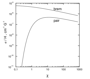
Figure 1: The total cross sections for magnetic bremsstrahlung and pair production as function of $\chi$.

The total probabilities (cross sections) for radiation and pair production for a given value of the magnetic field strength depend only on $\chi$ and are shown in figure 1. One can see that magnetic pair production has significant probability for $\chi\gtrsim 0.1$ (photon energy must be $\gtrsim 2mc^{2}$). For effective shower development one needs even higher values of $\chi$ ($\chi\gtrsim 1$) because with increasing $\chi$ the radiated photon spectrum becomes harder. For $\chi\gtrsim 1$ (quantum region) the energy of the radiated photon is of the order of the electron energy. It is interesting to note that for a photon with energy $\gtrsim 7,5\times 10^{19}\ \mathrm{eV}$ even Earth’s magnetic field ($\sim 0.3\ \mathrm{G}$) is strong enough ($\chi\sim 1$) to be a good environment for creating an electromagnetic shower. If such extremely high-energy photons are presented in the primary cosmic ray flux they will undergo cascading in the geomagnetic field before entering the Earth’s atmosphere. This problem has been intensively discussed recently in connection with the detection of the highest cosmic ray events [6].

As mentioned above, most of the treatments of cascades in a magnetic field were connected with specific models of astrophysical objects and are numerical in nature. The most general treatment of cascade properties emphasizing an analytical approach is made in [3], where the steady-state kinetic equations for the electron-positron and photon distributions are solved in a strong magnetic field.

A different approach to the shower study in a magnetic field is applied in [7]. It is similar to those for showers in matter and was motivated by the study of the primary gamma rays with extremely high energies ($\gtrsim 10^{20}\ \mathrm{eV}$) propagating through the geomagnetic field and Earth’s atmosphere. The average shower characteristics obtained by numerically solving the system of cascade equations, show some of the main features of the cascade. While the shower is similar to those in matter for $\chi\gg 1$, its nature changes sharply for $\chi\lesssim 1$ which is connected with sharp increase of the photon free path.

Recently, a kinetic theory of electromagnetic showers in a strong magnetic field has been developed in a similar to the cascade theory in matter, in approximation A [8]. Electromagnetic shower theories have been developed since 1937 following the works of Bhabha and Heitler and Carlson and Oppenheimer [9]. Landau and Rumer [10] developed a complete theory in approximation A. Their work contains the formalism which is widely used in later shower theories.

In the shower theory the mathematical description of the cascade process is based on the Boltzmann kinetic equation for particle flux density. The system of integro-differential equations of the one-dimensional Landau-Rumer theory is universal because it describes the shower development in any substance. Only the expressions for pair creation and bremsstrahlung probabilities per unit length are different. Using asymptotic forms of both processes for very high energies in a strong magnetic field, analytic formulae similar to those of standard cascade theory in approximation A for one-dimensional shower characteristics are obtained in [8]. But, as in matter, the kinetic equations were solved within certain approximations.

In this work we give the results from the Monte Carlo simulation of the longitudinal development of electromagnetic showers in a strong magnetic field for $\chi\gg 1$. We present shower profiles for different ratios of the primary and threshold energies, $E_{0}/E$, and energy spectra of shower particles at different depths. We analyse the behaviour of the shower maximum with respect to $E_{0}/E$. We compare our modelled results with theoretical ones in order to estimate theoretical approximations and the range of their validity.

2 The probability functions

The main elementary processes leading to particle multiplication in a magnetic field are magnetic bremsstrahlung and magnetic pair production. The corresponding probabilities per unit length are [8, 11]:

$$\pi\left(\varepsilon,\omega\right)\rmd\omega=\frac{\alpha m^{2}}{\pi\sqrt{3}}\frac{\rmd\omega}{\varepsilon^{2}}\left[\left(\frac{\varepsilon-\omega}{\varepsilon}+\frac{\varepsilon}{\varepsilon-\omega}\right)K_{\frac{2}{3}}\left(\frac{2u}{3\chi}\right)-\int\nolimits_{\frac{2u}{3\chi}}^{\infty}K_{\frac{1}{3}}\left(y\right)\rmd y\right]$$

(1)

$$\gamma\left(\omega,\varepsilon\right)\rmd\varepsilon=\frac{\alpha m^{2}}{\pi\sqrt{3}}\frac{\rmd\varepsilon}{\omega^{2}}\left[\left(\frac{\omega-\varepsilon}{\varepsilon}+\frac{\varepsilon}{\omega-\varepsilon}\right)K_{\frac{2}{3}}\left(\frac{2u_{1}}{3\chi}\right)+\int\nolimits_{\frac{2u_{1}}{3\chi}}^{\infty}K_{\frac{1}{3}}\left(y\right)\rmd y\right]$$

where $\varepsilon$ and $\omega$ are the electron and photon energy and $u=\frac{\omega}{\varepsilon-\omega}$, $u_{1}=\frac{\omega^{2}}{\varepsilon(\omega-\varepsilon)}$. Parameter $\chi$ was defined above. Here $\hbar=c=1$. $K_{\nu}\left(z\right)=\int\nolimits_{0}^{\infty}\rme^{-z\ \mathrm{ch}(t)}\mathrm{ch}\left(\nu t\right)\rmd t$ is a modified Bessel function known as MacDonald’s function. Parameter $\nu$ can have any real or complex values, here $\nu=\frac{2}{3}$ and $\frac{1}{3}.$ For simplicity we assume that the electron (positron) is moving perpendicular to the magnetic field $H$. As already mentioned, the probabilities of both processes are essentially different from zero under the condition that the parameter $\chi\gg 1$ , which means that the particle energy $\varepsilon>>\varepsilon_{c}$, where $\varepsilon_{c}=mc^{2}\frac{H_{cr}}{H}$. It is mentioned in [11] that this condition corresponds to the conditions $u/\chi<<1$ and $u_{1}/\chi<<1$, i.e. one can use in (1) the asymptotic form of $K_{\nu}\left(z\right)$ for $z<<1$, $K_{\nu}(z\ll 1)=\frac{\Gamma(\nu)}{2^{1-\nu}}(\frac{1}{z})^{\nu}+...$. Then expressions (1) may be simplified:

$$\pi\left(\varepsilon,\omega\right) = q\left[\frac{\left(\varepsilon-\omega\right)^{\frac{5}{3}}}{\varepsilon^{\frac{7}{3}}\omega^{\frac{2}{3}}}+\frac{1}{\left(\varepsilon-\omega\right)^{\frac{1}{3}}\varepsilon^{\frac{1}{3}}\omega^{\frac{2}{3}}}\right],$$

$$\gamma\left(\omega,\varepsilon\right) = q\left[\frac{\left(\omega-\varepsilon\right)^{\frac{5}{3}}}{\omega^{\frac{8}{3}}\varepsilon^{\frac{1}{3}}}+\frac{\varepsilon^{\frac{5}{3}}}{\omega^{\frac{8}{3}}\left(\omega-\varepsilon\right)^{\frac{1}{3}}}\right],$$

where $q=3.9\times 10^{6}\left[\frac{H}{H_{c}}\right]^{\frac{2}{3}}\frac{\mathrm{GeV}^{\frac{1}{3}}}{\mathrm{cm}}$. Using $u=\omega/\varepsilon$ (correspondingly $u=\varepsilon/\omega$) we can rewrite (LABEL:eq2) in the form:

$$\pi\left(\varepsilon,\omega\right)d\omega = \frac{q}{\varepsilon^{\frac{1}{3}}}\left[\frac{\left(1-u\right)^{\frac{5}{3}}}{u^{\frac{2}{3}}}+\frac{1}{\left(1-u\right)^{\frac{1}{3}}u^{\frac{2}{3}}}\right]\rmd u,$$

$$\gamma\left(\omega,\varepsilon\right)d\varepsilon = \frac{q}{\omega^{\frac{1}{3}}}\left[\frac{\left(1-u\right)^{\frac{5}{3}}}{u^{\frac{1}{3}}}+\frac{u^{\frac{5}{3}}}{\left(1-u\right)^{\frac{1}{3}}}\right]\rmd u.$$

The total probabilities per unit length for bremsstrahlung and pair production are given by

$$W_{r}\left(\varepsilon\right) = \int\nolimits_{0}^{\varepsilon}\pi\left(\varepsilon,\omega\right)\rmd\omega=\frac{q}{\varepsilon^{\frac{1}{3}}}\int\nolimits_{0}^{1}\left[\frac{\left(1-u\right)^{\frac{5}{3}}}{u^{\frac{2}{3}}}+\frac{1}{\left(1-u\right)^{\frac{1}{3}}u^{\frac{2}{3}}}\right]\rmd u$$ (4)

$$= 5.642\frac{q}{\varepsilon^{\frac{1}{3}}},$$

$$W_{p}\left(\omega\right) = \int\nolimits_{0}^{\omega}\gamma\left(\omega,\varepsilon\right)\rmd\varepsilon=1.467\frac{q}{\omega^{\frac{1}{3}}}.$$ (5)

Unlike the Bethe-Heitler probability,$\ \pi(\varepsilon,\omega)$ does not contain an infrared divergence and because of this $W_{r}\left(\varepsilon\right)$ is finite.

As mentioned earlier, the probabilities of both processes were obtained using the asymptotic form of the function $K_{\nu}\left(z\right)$ for $z<<1$. This explains the behaviour of the total cross sections as a function of the particle energy of power $(-\frac{1}{3})$ (at fixed $H$) and in figure 1 this is the region of $\chi\gg 1$. Expression (5) coincides with the expression of the photon attenuation coefficient given in Erber’s review [5] when the asymptotic form of auxiliary function $T(\chi)$ for $\chi>>1$, $T(\chi)\sim 0.60\chi^{\frac{1}{3}}$, is used. Here $\chi=\frac{1}{2}\frac{h\nu}{mc^{2}}\frac{H}{H_{cr}}$, $h\nu$ is the photon energy.

3 Simulation

To investigate the shower characteristics in a strong magnetic field we developed our own Monte Carlo code. The probabilities (LABEL:eq3) were used to sample energies of the secondary particles - photon in bremsstrahlung and electron in pair creation. We constructed tables with cumulative distributions from probabilities (LABEL:eq3) through a small step by $u$. The mean interaction length is the inverse value of the total probability, (4) and (5).

It was shown in [8] that the average ranges of both electron and photon, with energy $E_{0}$ in a magnetic field $H$, are of the same order of magnitude, $\sim\frac{E_{0}^{\frac{1}{3}}}{q}$. The quantity $L=\frac{E_{0}^{\frac{1}{3}}}{q}$ which includes the matter parameters (magnetic field strength $H$) could play the role of a radiation length. In this case $E_{0}$ is the energy of the particle initiating the shower. It is important to note, that unlike matter, here $L$ depends on the energy $E_{0}$ of the primary particle. $L$ is a relatively small quantity. For example, in magnetic field $H=10^{5}\ \mathrm{G}$  for $E_{0}=10^{6}\ \mathrm{GeV}$, $L=14.86\ \mathrm{cm}$, for $E_{0}=10^{9}\ \mathrm{GeV}$, $L=148.6\ \mathrm{cm}$.

We considered the problem as one dimensional, i.e. we assumed that the shower is only developing in the direction of the primary particle entering the magnetic field at $t=0$. The distance is measured in units $L$. All shower particles were followed down to some threshold energy $E$.

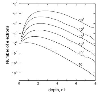
Figure 2: Shower profiles for electron induced showers. Numbers refer to the ratio $E_{0}/E$.

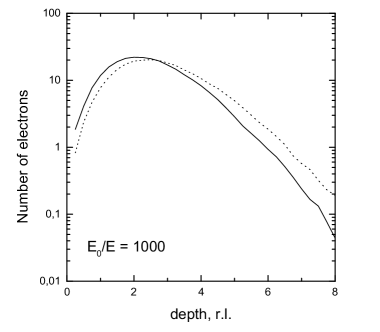
Figure 3: Shower profiles for electron (solid curve) and photon (dashed curve) induced showers.

4 Results and discussion

We performed simulation for various sets of primary and threshold energies ($E_{0}$ and $E$) and different magnetic field strengths $H.$

Our results confirmed the theoretical prediction that the above-mentioned quantity, $L$, plays the role of a radiation length. Similar to the standard shower theory under approximation A, the longitudinal cascade development is independent of an absorber (magnetic field) when distances are measured in radiation lengths and the average behaviour of a shower is expressed by a function of $E_{0}/E.$

Shower profiles for electron-initiated showers and different $E_{0}/E$ are shown in figure 2. The corresponding curves for photons are very close to those of electrons and because of this they are not shown. When the primary particle is a photon (figure 3), the shower maximum is shifted by $\sim\frac{1}{2}\ \mathrm{r.l.}$ (where r.l. denotes radiation length) deeper, which is close to the difference between the mean interaction lengths of primary electron and photon.

The differential energy spectra of shower particles at different stages of the shower development are shown in figure 4. The depth of $2.25\ \mathrm{r.l}$. is near the shower maximum. The spectra can be described by power-law of energy, $E\frac{\rmd n}{\rmd E}\sim E^{-\delta}$, with $\delta$ increasing with the depth and approaching $1$ for $t\rightarrow\infty$.

As can be seen, the typical distance over which the shower develops is a few radiation lengths. The depth of the shower maximum increases very slowly with the increase of $E_{0}/E$ approaching a limit. In very strong fields, e.g. in pulsars, $L$ becomes very small ($\sim 10^{-4}\ \mathrm{cm}$ for $E_{0}=10^{6}\ \mathrm{GeV}$) which means that the shower has the longitudinal spread of the same order. This confirms the theoretical prediction in [8] that the strong magnetic fields are effective screens for very high energy electrons, positrons and photons.

Figure 4: Energy spectrum of electrons at three depths: line with squares-$0.75\ \mathrm{r.l.}$, line with circles-$2.25\ \mathrm{r.l}$. (near the shower maximum), line with crosses-$5\ \mathrm{r.l.}$ $E_{0}/E=1000$.

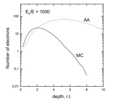
Figure 5: Simulated shower profile (MC) compared with the theoretical curve in the adiabatic approximation (AA).

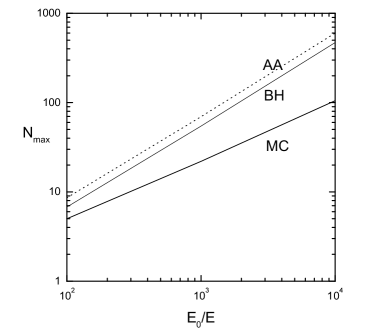
Figure 6: The number of electrons in the shower maximum as a function of $E_{0}/E$. MC-this work, AA-adiabatic approximation and BH-classical cascade theory in approximation A.

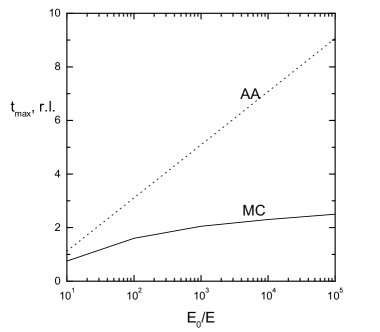
Figure 7: Depth of the maximum as a function of $E_{0}/E$.

It should be noted here that these properties of the shower are valid for such values of $E_{0}$, $E$ and $H$ that satisfy the condition $\chi\gg 1$ and the asymptotic expressions (2) can also be used. In addition, to consider the shower as one-dimensional, the electron energies must obey the condition [8]

$$\left(\frac{\varepsilon}{mc^{2}}\right)^{\frac{2}{3}}\left(\frac{H_{cr}}{H}\right)^{\frac{1}{3}}\frac{\alpha}{2\pi}\gg 1.$$

This criteria comes from the requirement that the electron gyroradius $R=\varepsilon/eH$ must be much greater than the typical length of the shower, i.e. $R\gg L$.

However, detailed comparison of a numerical results shows that the Monte Carlo cascade curves differ significantly from the theoretical ones. This is illustrated in figure 5 where shower profiles for the electron-induced showers and $E_{0}/E=1000$ are shown.

This disagreement could probably be explained with the approximations used in [8] to get a solution of cascade equations. In the case of a magnetic field, the shower theory is more complicated than the conventional theory in approximation A because the probabilities $\pi\left(\varepsilon,\omega\right)\rmd\omega$ and $\gamma\left(\omega,\varepsilon\right)\rmd\varepsilon$ are not scaling functions, i.e. they do not depend only on the ratio of secondary to primary energies (functions of $\omega/\varepsilon\;$or $\varepsilon/\omega$ in our notation). Mellin transforms lead to differential-difference equations for the distribution functions and its solutions are found by authors of [8] in the so-called adiabatic and modified adiabatic approximations. As pointed out in [8], the adiabatic approximation (AA) is limited to the region after the maximum. In the modified adiabatic approximation it is assumed that the explicit dependence of $\pi\left(\varepsilon,\omega\right)$ and $\gamma\left(\omega,\varepsilon\right)$ on primary energy can be eliminated by its substitution with some mean energy per interaction in the shower. This leads to the same solutions with the modified radiation length but, obviously, the shower development is distorted. If we use the probabilities $\pi\left(\varepsilon,\omega\right)$ and $\gamma\left(\omega,\varepsilon\right)$ in this modified way in our Monte Carlo code we obtain results very close to the theoretical ones. Figure 6 shows the number of electrons in the shower maximum $N_{\max}$ as function of $E_{0}/E$. One can see that the rise of $N_{\max}$ with $E_{0}/E$ is slower than that of AA of the theory. $N_{\max}$ is exactly proportional to $\left(E_{0}/E\right)^{\xi}$ . AA gives $\xi$ close to one as it is in the standard theory with Bethe-Heitler cross sections (curve labelled BH in the figure) while our simulation (curve labelled MC) gives $\xi\approx\frac{2}{3}$. Figure 7 shows the depth of the maximum $t_{\max}$ as a function of $E_{0}/E$ for both theoretical and simulated showers. As can be seen, the behaviour of the modelled $t_{\max}$ is too different from those of logarithmically increasing theoretical $t_{\max}$. After some $E_{0}/E$ the modelled $t_{\max}$ almost ceases to increase.

It is easy to demonstrate this feature of showers in a magnetic field using Heitler’s elementary cascade model [12]. In this model, electromagnetic particles subdivide into two particles with half the initial energy. In matter this takes place on every radiation length. In a magnetic field, however, the situation is substantially different. After each interaction the interaction length, which is a function of energy power of $\frac{1}{3}$, decreases due to particle energy splitting. If the primary particle has an energy $E_{0}$ and the interaction length $t_{0}\ \mathrm{r.l.}$, then after the first interaction the number of particles will be two, each of energy $E_{0}/2$. The next interaction length will be $t_{0}/2^{\frac{1}{3}}$ and the number of particles four, each of energy $E_{0}/4$. After $N$ interactions the particle number is already $2^{N}$ and their energy $E=E_{0}.2^{-N}$. The next interaction length will be $\frac{t_{0}}{\left[2^{\frac{1}{3}}\right]^{N}}\ \mathrm{r.l.}$ The distance at which this takes place is

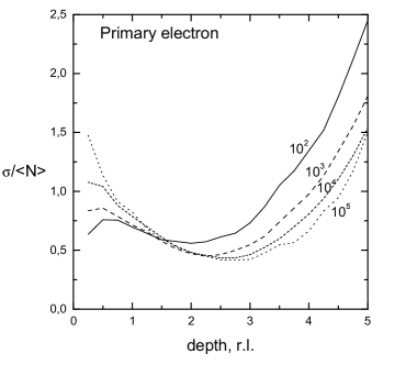
Figure 8: Fluctuations of the number of electrons $\left(\sigma/\langle N\rangle\right)$ as a function of the depth for different $E/E_{0}$.

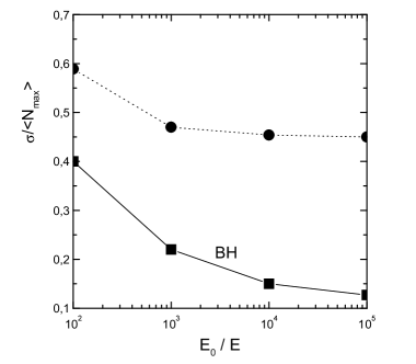
Figure 9: Fluctuations of the number of electrons in the shower maximum $\left(\sigma/\langle N\rangle\right)$ as a function of $E/E_{0}$. Dotted line-showers in a magnetic field, solid line-BH showers.

$$T=t_{0}+\frac{t_{0}}{2^{\frac{1}{3}}}+\frac{t_{0}}{\left(2^{\frac{1}{3}}\right)^{2}}+...+\frac{t_{0}}{\left(2^{\frac{1}{3}}\right)^{N-1}}=t_{0}\left[1+\frac{1}{2^{\frac{1}{3}}}+\frac{1}{\left(2^{\frac{1}{3}}\right)^{2}}+...+\frac{1}{\left(2^{\frac{1}{3}}\right)^{N-1}}\right].$$

The expression in the square brackets is a sum of a geometrical progression with $q=2^{-1/3}$ and thus

$$T = 4.847t_{0}\left[1-\frac{1}{\left(2^{\frac{1}{3}}\right)^{N-1}}\right].$$ (6)

This expression shows that if $N$ increases, i.e. $E_{0}/E$ increases, $t_{\max}$ approaches a limit. This means that after some $N$ (or $E_{0}/E$) $\ t_{\max}$ practically ceases to increase. In our rather simplified model the maximum $t_{\max}\$is $4.847t_{0}\ \mathrm{r.l.}$ The first interaction length $t_{0}$ is $0.117\ \mathrm{r.l}$. for the electron and $0.682\ \mathrm{r.l.}$ for the photon. If we take the greater value this will lead to an estimation of the maximum $t_{\max}$ of $3.31\ \mathrm{r.l.}$ whose value does not contradict with the curve modelled in figure 7.

Another important characteristic of electromagnetic showers in a strong magnetic field which can be easily obtained from the simulation are fluctuations in the shower development. There is no theoretical consideration of this problem. The problem is complicated even for the standard cascade theory (see, e.g. [13]).

In figure 8 the fluctuations of the number of shower electrons $\left(\sigma/\langle N\rangle\right)$ as a function of the depth for different $E_{0}/E$ are shown. The primary particle is an electron. The behaviour of the curves is very similar to those of BH showers but the fluctuations in a magnetic field are significantly larger. This is illustrated in figure 9 where fluctuations in the shower maximum as a function of $E_{0}/E$ are shown, compared with BH showers. Calculations for BH showers are performed by direct MC simulation in air for very high energies $E_{0}$ and $E$, i.e. at the conditions where the standard cascade theory in approximation A is valid.

The larger fluctuations in a magnetic field compared to BH showers are not an unexpected result. The main sources for the fluctuations of the number of particles in the cascade are fluctuations of interaction lengths and the random energy distribution of created secondary particles. Unlike the BH cross sections the mean interaction lengths for magnetic bremsstrahlung and pair-production processes are functions of the particle energy of power $\frac{1}{3}$ (see (4,5)). The differential cross sections (LABEL:eq3) depend on the particle energy as well. Their features lead to a significant probability that the secondary electron or photon will take a large fraction of the primary energy.

5 Conclusions

A direct MC simulation of the longitudinal development of electromagnetic showers in a strong magnetic field has been performed. The processes of the magnetic bremsstrahlung and of the magnetic pair production were included in the simulation with asymptotic expressions for both probabilities valid for very high energies. Simulated results were compared with the theory of showers in a strong magnetic field developed in [8]. The main predictions of this theory - the dependence of the radiation length on magnetic field strength and the energy of the primary particle, the very small shower longitudinal spread and the closeness of electron and photon profiles, are confirmed by our simulation.

However, the AA of the theory used in [8] was inadequate for a precise qualitative estimate of shower characteristics.

References

References

- [1] Sturrock P A 1971 Ap.J. 164 529
- [2] Daugherty J K and Harding A 1982 Ap.J. 252 337
- [3] Baring M 1989 Astron. Astrophys. 225 260
- [4] Bednarek W 1997 Mon. Not. R. Astron. Soc. 285 69
- [5] Erber T 1966 Rev. Mod. Phys. 38 626
- [6] Halzen F, Vazquez R, Stanev T and Vankov H P 1995 Astrophys. Phys. 3 151
- [7] Kanevsky B L and Goncharov A I 1989 Voprosy atomnoy nauki i techniki. Seria: Technika fiz. exp. 4 1 (in Russian)
-
[8]
Akhiezer A I, Merenkov N P and Rekalo A P 1994 J. Phys. G: Nucl. Part. Phys. 20 1499
Akhiezer A I, Merenkov N P and Rekalo A P 1995 Nucl. Phys. 58 491 (in Russian) -
[9]
Bhabha H J and Heitler W 1937 Proc. R. Soc. A
519 432
Carlson J F and Oppenheimer J R 1937 Phys. Rev. 51 220 - [10] Landau L and Rumer G 1938 Proc. R. Soc. A 166 213
- [11] Bayer V H, Katkov B M and Fadin V S 1973 Radiation of Relativistic Electrons (Moscow: Atomizdat) (in Russian)
- [12] Rossi B 1952 High Energy Particles (New York)
- [13] Uchaikin V V and Ryzhkov V V 1998 Stochastic Theory of High Energy Particle Transfer (Novosibirsk: Nauka) (in Russian)