Abstract

In this paper we discuss various possibilities of using X-ray observations to gain information about the large-scale structure of the Universe. After reviewing briefly the current status of these investigations we explore different ways of making progress in this field, using deep surveys, large area surveys and X-ray background observations.

Clustering in the X-ray Universe

¹Instituto de Física de Cantabria (CSIC-UC), 39005 Santander, Spain
²Mullard Space Science Laboratory, University College London, UK
³Departamento de Física Moderna, Universidad de Cantabria, 39005 Santander, Spain

1 Introduction

X-ray emission in the Universe arises in intense gravity environments. At high galactic latitudes, active galactic nuclei (AGN) and other emission line galaxies dominate the source counts at all explored fluxes, with galaxy clusters being the second most abundant source class.

Recent ROSAT deep surveys ([1], [2], [3]) have shown that most of the soft X-ray volume emissivity in the Universe arises at redshifts $z>1-2$ ([4]). The AGN and star formation rate per unit volume follow a remarkably similar evolution rate in the Universe ([5]) and therefore they can both be used as tracers of the evolution of large-scale structure in the Universe. Using AGN and star-forming galaxies as tracers of cosmic inhomogeneities is most sensitive to intermediate redshifts ($z\sim 2$), providing a critical link between cosmic microwave background studies (which map the $z\sim 1000$ Universe) and local galaxy surveys ($z\sim 0$).

In this paper we briefly review the current status of the use of X-ray observations towards the study of large-scale structure. More details are presented in [29]. Then we explore possibilities of making qualitative progress in this field by carrying out different types of X-ray surveys.

2 What we know so far

At galactic latitudes $\mid b\mid>20^{\circ}$ the contribution from the Galaxy to the X-ray sky is small: less than 10% of the X-ray background above 2 keV is due to galactic emission, absorption is negligible above this photon energy and a census of X-ray sources down to any flux limit exhibits less than 10-20% of galactic stars. Observations of the X-ray background at high galactic latitudes and photon energies above 2 keV can therefore be used to map the extragalactic X-ray sky.

2.1 The isotropy of the X-ray background

The all-sky distribution of the X-ray background for cosmological purposes has been best mapped by the HEAO-1 mission. A galactic anisotropy dominates the large-scale anisotropy, but this can be modelled out ([6]). A dipole contribution is detected in the X-ray sky, in rough alignment with the direction of our motion with respect to the Cosmic Microwave Background frame ([7], [8]). The amplitude of this dipole accounts for both the kinematical effect of our motion (the Compton-Getting effect) and the excess X-ray emissivity associated with the structures which are pulling us. These two effects are expected to be of the same order ([9]) and the analysis done in [8] shows this to be the case. However, in an analysis of the ROSAT all-sky data at lower photon energies (which have the disadvantage of a larger contamination from the Galaxy) Plionis & Georgantopoulos [10] find a dipole several times larger than the expected kinematical dipole. The difference between both results might be partly affected by the elimination of X-ray bright clusters in the Scharf et al analysis, as clusters are known to be a largely biased population ([11]). The bias parameter derived from the XRB dipole is large ($b_{X}\sim 3-6$).

Treyer et al [12] have analyzed higher order multipoles of the HEAO-1 A2 X-ray background. The discrete nature of the XRB contributes a constant term to all multipoles which scales as $\propto S_{cut}^{0.5}$, where $S_{cut}$ is the minimum flux at which sources have been excised. Treyer et al detect a signal growing towards lower-order multipoles which is consistent with a gravitational collapse picture, as predicted by [9]. Excluding the dipole, this analysis yields a moderate bias parameter for the X-ray sources ($b_{X}\sim 1-2$).

On smaller (a few degrees) angular scales, probing linear scales of hundreds of Mpc, the ‘excess fluctuations’ technique has been used often in the analysis of the XRB. The way this works is by modelling the distribution of XRB intensities on a given angular scale in terms of confusion noise, plus a contribution coming from source clustering ([13]). These studies have yielded so far only upper limits for the excess fluctuations: $<2\%$ on scales of $5^{\circ}\times 5^{\circ}$ ([14]) and $<4\%$ on scales $1^{\circ}\times 2^{\circ}$ ([15]). We discuss later what is the expected signal and how it could be measured.

Yet on smaller (a few arcmin) angular scales, which probe the galaxy-galaxy clustering scale, data from X-ray imaging telescopes has been used. The autocorrelation function of the XRB on these scales should reflect the clustering of high redshift X-ray sources in the nonlinear regime ([16]). Soltan et al [17] have found a strong positive detection for angular separations 0.3-20^∘ which is, however, difficult to interpret as both the Galaxy and the Local Supercluster could contribute to this.

2.2 Clustering of X-ray selected AGN

Studying the clustering of X-ray selected AGN is likely to be the most direct way to map the structure of the X-ray sky. At soft X-ray energies this requires fairly deep surveys (going below $\sim 10^{-14}\,{\rm erg}\,{\rm cm}^{-2}\,{\rm s}^{-1}$) as otherwise very few objects at $z>1$, where most of the X-ray volume emissivity is produced, would be sampled.

Carrera et al [18] have analysed a set of ‘pencil beam’ medium and deep ROSAT images containing 200 X-ray selected AGN, sampling a redshift interval $z\sim 0-2$. The net result is the detection of X-ray selected AGN clustering which is relatively weak (the 3D correlation length is $r_{0}<5\,h^{-1}\,{\rm Mpc}$, for $h=H_{0}/(100\,{\rm km}\,{\rm s}^{-1}\,{\rm Mpc}^{-1})$) and strongly evolving with redshift (faster than comoving). At much brighter flux limits [19] used the ROSAT All Sky Survey Sources to derive a 2D correlation function that, when translated to 3D with an appropriate catalogue depth, yields a larger correlation length ($r_{0}\sim 6\,h^{-1}\,{\rm Mpc}$).

2.3 Do X-rays trace mass?

In [29] we compile various measurements of the bias parameter for X-ray sources and in particular for X-ray selected AGN and the XRB. The bias parameter is likely to be redshift dependent. For a simple model where all objects form at the same early redshift, Fry [20] finds $b_{X}(z)=b_{X}(0)+z(b_{X}(0)-1)$, which implies that at high z the bias parameter could be large.

The other effect that comes into play, especially when using the XRB, is that at low redshift clusters become more numerous and their imprint in the local XRB features becomes more important. As clusters are a strongly biased source population ([11] estimate $b_{X}(0)\sim 4$) it is not surprising that the amplitude of the XRB dipole calls for large bias factors, but higher order multipoles (sensitive to more distant sources) do not.

Within present knowledge and uncertainties, the bias factor for the AGN as the dominant X-ray source population, appears to take moderate values $b_{X}=1-2$ at low to intermediate redshifts. Indeed at higher redshifts the AGN population might be more strongly biased.

3 Deep hard X-ray surveys

Deep surveys, particularly at hard photon energies, are a key ingredient to forthcoming studies af the large-scale structure of the X-ray Universe. Currently popular models for the X-ray background assume a population of AGN with a distribution of absorbing columns ([21], [22], [23]), where most of the X-ray energy produced by accreting black holes is absorbed and re-radiated in the infrared ([24], [25]). Several claims have been made that the absorbed AGN population evolves differently than the unabsorbed one ([26], [30], [31]). As most of the energy content in the XRB resides at 30 keV, it is crucial to explore harder photon energies than previously achieved with the ROSAT deep surveys.

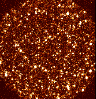
Figure 1: Simulation of a 2-10 keV deep XMM EPIC pn image of 350 ks

XMM is the most sensitive X-ray observatory to survey the X-ray sky at photon energies above 2 keV. Although its point-spread-function is significantly worst than that of Chandra, at energies above 2 keV both instruments are photon-starved and then the much larger collecting area of XMM will make it more efficient. We have carried out extensive simulations of XMM EPIC observations at various depths and found that the deepest planned XMM observations (PVCal, GTO and AO-1) reaching  350-400 ks will not be confusion noise limited. Figure 1 shows the resulting image in the 2-10 keV band of a simulation of a 350 ks XMM EPIC-pn exposure in a blank field (using the standard model [23]). As the EPIC field of view is $\sim 30^{\prime}$ in diameter, we expect to find $\sim 300$ sources in such a pointing once vignetting has been corrected for. Most of these sources are expected to lie at redshifts $z>1-2$, from which the X-ray volume emissivity in hard X-rays will be derived and compared with the one, assumed so far, obtained with ROSAT for soft X-ray photons.

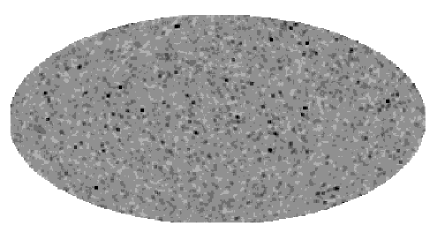
Figure 2: Simulation of a 4-12 keV X-ray background map (ignoring the galaxy), as observed with a 1 $m^{2}$ collimator with a field of view of 1$\deg^{2}$, scanning the sky for 6 months 100% efficiency.

4 X-ray background surveys

The measurement of large-scale structure in the X-ray Universe does not necessarily require individually resolving all sources in very large areas of the sky down to very faint fluxes. If the X-ray volume emissivity as a function of $z$ can be derived from deep surveys, fluctuation analyses of the XRB can also be used ([27]). If the X-ray volume emissivity peaks at some intermediate redshift as it does in soft X-rays ($z\sim 1-2$), then for a fixed angular scale the XRB fluctuations are related almost uniquely to the value of the power spectrum of the inhomogeneities in the Universe at a single comoving wavenumber. The scales to be probed by XMM (from a few to a few tens of arcmin) will provide a measurement of the $k\sim(0.1-1)h{\rm Mpc}^{-1}$ regime. The power spectrum is expected to peak at $k\sim 0.05h{\rm Mpc}^{-1}$, which corresponds to an angular scale of $\sim 1\deg$.

In [27] we argue that to detect the excess fluctuations of the XRB due to source clustering for a beam size of 1$\deg^{2}$, a large fraction of the sky needs to be surveyed. To prove that this is feasible, we have carried out simulations of hard X-ray source populations over the whole sky with a simple clustering model for the sources and measured XRB intensities (details in [27]). These intensities are then ‘measured’ with a proportional counter of 1m² effective area during one complete 6-month scan of the sky at 100% efficiency and including stable particle background in a manner similar to the Ginga LAC observations.

Figure 3: Intensity distributions for the map in Fig 2. (ignoring $\mid b\mid<20^{\circ}$) for no clustering (continuous line), linear evolution of clustering (dashed line) and comoving clustering evolution (dotted line).

Figure 2 shows one of these simulations where the clustering has been modeled with a gaussian correlation function with comoving evolution. Ignoring data within $\mid b\mid<20^{\circ}$, Figure 3 shows the histograms for the XRB intensities in 3 cases: absence of clustering, linear clustering evolution and comoving clustering evolution ($b_{X}=1$ in all cases). The distributions are clearly distinguishable, and the excess fluctuations can be determined with a very high accuracy. Indeed with a significantly smaller collecting area and similar circumstances, excess fluctuations can still be detected, but measured with larger statistical uncertainties.

One such survey will also benefit other approaches to measure large-scale structure in the Universe, particularly the multipole expansion, especially if a sensitive source survey could also be carried out. In this way, those $1\deg^{2}$ regions where sources above a given flux are detected could be masked out for the multipole analysis, as discussed in [12].

5 Large-area surveys

Direct measurements of the large-scale structure of the Universe at redshifts $z\sim 1-2$ via X-ray observations require surveying areas of hundreds of square degrees to a sufficient depth. Using galaxy clusters as tracers of large-scale structure of the Universe presents the difficulty of the faintness of most of these objects beyond redshifts $z\sim 1$. Even XMM will require a large amount of time to do a sensible mapping of galaxy clusters out to these redshifts.

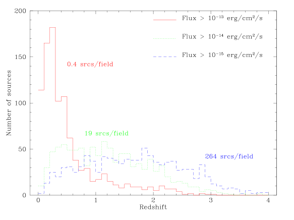
Figure 4: Redshift distribution of AGN for different 2-10 keV flux limits.

Using AGN has the advantage that they have strong positive evolution up to $z\sim 1-2$. In order to reach the redshifts where most of the X-ray emissivity is produced $z\sim 1-2$, AGN surveys have to go down to, at least, a 2-10 keV flux $\sim 10^{-14}\,{\rm erg}\,{\rm cm}^{-2}\,{\rm s}^{-1}$. Figure 4 illustrates the redshift distribution for different flux limits assuming the [23] model. The advantage of X-ray AGN surveys over similar optical work (e.g. the Sloan Digital Sky Survey) is that with hard X-rays the absorbed AGNs can also be used up to earlier times if they evolve more strongly than the unabsorbed broad-line objects.

Mapping a 100$\deg^{2}$ contiguous area of the sky with the XMM EPIC cameras, which have the largest field of view among all operating X-ray facilities, to a depth of $\sim 20ks$ (needed to get reliable detections at $>10^{-14}\,{\rm erg}\,{\rm cm}^{-2}\,{\rm s}^{-1}$) will require 10 Msec of effective exposure time with XMM. This will collect $\sim 10^{5}$ sources.

A more efficient way to carry out that project is by means of a dedicated mission with a wide-field X-ray telescope. The Panoram-X mission proposed in [28], would cover the whole sky to a depth $\sim 10^{-14}\,{\rm erg}\,{\rm cm}^{-2}\,{\rm s}^{-1}$. Of course, finding redshifts for a reasonable fraction of the several tens of millions of sources to be discovered by such mission is simply impossible. A full analysis of the spatial distribution of X-ray selected AGN would then require the modelling of the 2D distribution from these maps, using redshift distributions from the deep hard X-ray surveys.

6 Outlook

X-ray cosmology is just in its infancy. Basic questions such as what is the bias parameter of different classes of X-ray sources are still partly unanswered. However the fact that most of the X-ray sky is dominated by extragalactic sources of which AGN are the major component make the X-ray sky especially suited for cosmology at intermediate redshifts.

Making quantitative progress in this field requires not only proper use of existing or planned observatory-type facilities (i.e., Chandra and XMM), but probably also dedicated missions to survey all (or most of) the sky. X-ray cosmology is now in a position to make specific predictions for the structure of the X-ray universe (once hard X-ray surveys have been carried out with Chandra and XMM). These surveys can then be designed and optimized to obtain detections and precise measurements of the large-scale structure of the Universe at redshifts $z\sim 1-2$. That would really be a major boost for cosmology at intermediate redshifts.

References

- [1] Boyle, B.J. et al, 1994, MNRAS, 271, 639
- [2] McHardy, I.M., et al 1998, MNRAS,
- [3] Hasinger, G. et al 1998, A&A, 329, 482
- [4] Miyaji, T., Hasinger, G., Schmidt, M., 1999, A&A, in press
- [5] Franceschini, A., Hasinger, G., Miyaji, T., Malquori, D., 1999, MNRAS, in the press, (astro-ph/9909290)
- [6] Iwan, D. et al, 1982, ApJ, 260, 111
- [7] Shafer, R.A., 1983, PhD thesis, Univ of Maryland
- [8] Scharf, C., et al, 1999, ApJ, submitted
- [9] Lahav, O., Piran, T., Treyer, M.A., 1997, MNRAS, 284, 499
- [10] Plionis, M., Georgantopoulos, I., 1999, MNRAS, in the press
- [11] Plionis, M., Kolokotronis, V., 1998, ApJ, 500, 1
- [12] Treyer, M., et al, 1998, ApJ, 509, 531
- [13] Barcons, X., 1992, ApJ, 396, 460
- [14] Shafer, R.A., Fabian, A.C., 1983, in: IAU Symposium 104, Early evolution of the Universe and its present structure, Reidel, p. 333
- [15] Butcher, J.A. et al, 1997, MNRAS, 291, 437
- [16] Carrera, F.J., Barcons, X., 1992, MNRAS, 257, 507
- [17] Soltan, A. et al 1999, A&A, 349, 354
- [18] Carrera, F.J. et al 1998, MNRAS, 299, 229
- [19] Akylas, A., Georgantopoulos, I., Plionis, M., 1999, MNRAS, submitted (astro-ph/9911254)
- [20] Fry, J.N., 1996, ApJ, 461, L65
- [21] Setti, G., Woltjer, L., 1989, A&A, 224, L21
- [22] Madau, P., Ghisellini, G., Fabian, A.C., 1994, MNRAS, 270, L17
- [23] Comastri, A., Setti, G., Zamorani G., Hasinger, G., 1995, A&A, 296, 1
- [24] Fabian, A.C. et al, 1998, MNRAS, 297, L11
- [25] Fabian, A.C., Iwasawa, K., 1999, MNRAS, 303, L34
- [26] Gilli, R., Risalati, G., Salvati, M., 1999, A&A, in the press (astro-ph/9904422)
- [27] Barcons, X., Fabian, A.C., Carrera, F.J., 1998, MNRAS, 293, 60
- [28] Chincarini, G., 1999, preprint (astro-ph/9902184)
- [29] Barcons, X., Carrera, F.J., Ceballos, M.T., Mateos, S., 2000, Astrophys Lett & Comm, submitted
- [30] Pompilio, F., La Franca, F., Matt, G., 2000, A&A, in the press (astro-ph/9909390)
- [31] Fabian, A.C., 2000, MNRAS, in the press (astro-ph/9908064)