On energy-dependent propagation effects and acceleration sites of relativistic electrons in Cassiopeia A

Abstract

We consider the effect of energy dependent propagation of relativistic electrons in a spatially inhomogeneous medium in order to interpret the broad-band nonthermal radiation of the young shell-type supernova remnant (SNR) Cassiopeia A. A two-zone model is proposed that distinguishes between compact, bright steep-spectrum radio knots and the bright fragmented radio ring on the one hand, and the remainder of the shell - the diffuse ‘plateau’ - on the other hand. In the framework of this model it is possible to explain the basic features of the spectral and temporal evolution of the synchrotron radiation of Cas A if one assumes that these compact structures correspond to sites of efficient electron acceleration producing hard spectra of accelerated particles with power-law indices $\beta_{\rm acc}\sim 2.2$. The resulting energy distribution of radio electrons in these compact structures becomes significantly steeper than the electron production spectrum on timescales of the energy dependent escape of these electrons into the surrounding diffuse plateau region. We argue that the steepness, rather than the hardness, of the radio spectra of compact bright structures in clumpy sources can in general be considered as a typical signature of sites where strong electron acceleration has built up high gradients in the spatial distribution of radio electrons. Subsequent diffusive escape then modifies their energy distribution, leading to potentially observable spatial variations of spectral indices within the radio source. Qualitative and quantitative interpretations of a number of observational data of Cas A are given. Predictions following from the model are discussed.

1 Introduction

Cassiopeia A is the youngest of the known galactic supernova remnants (SNRs) whose birth probably dates back to 1680 (Ashworth ashworth (1980)). It is one of the most prominent and well studied radio sources on the sky (e.g. Bell et al. bell75 (1975); Tuffs tuffs86 (1986); Braun et al. braun (1987); Anderson et al. arlpb (1991) – hereafter ARLPB; Kassim et al. kassim (1995), hereafter KPDE; etc.), whose synchrotron radiation probably extends into the hard X-ray region (Allen et al. allen (1997); Favata et al. favata (1997)). Most of the radiation of both nonthermal and thermal origin comes from a shell region enclosed between two spheres, with angular radii $\simeq 150\,\rm arcsec$ and $\simeq 100\,\rm arcsec$, corresponding to spatial radii $R_{0}=2.5\,\rm pc$ and $R_{\rm ring}=1.7\,\rm pc$, respectively, for a distance of $d\approx 3.4\,\rm kpc$ (Reed et al. reed (1995)). The former corresponds to the mean radius of the assumed blast wave, while the latter is supposedly the mean radius of the reverse shock in the freely expanding (upstream) ejecta which are heating the gas to temperatures $\sim\!(1-3)\,\rm keV$, thus creating the hot thermal X-ray component (Becker et al. becker (1979); Fabian et al. fabian (1980); Jansen et al. jansen (1988)).

Cas A is considered to be a powerful particle accelerator, with an energy content in relativistic electrons, estimated from simple equipartition arguments, in the range $W_{\rm e}\sim 10^{48}-5\times 10^{49}\,\rm erg$ (e.g. Chevalier et al. chevetal (1978); ARLPB ). This value should be increased by more than an order of magnitude for the total energetics in relativistic particles if the high ratio between relativistic protons and electrons observed in cosmic rays (CR) holds in Cas A. However, the mechanisms and sites of particle acceleration in Cas A have not yet been identified.

Observations of Cas A at optical wavelengths show strong line emission from 2 main types of compact structures. The quasi stationary flocculi are thought to trace the circumstellar medium (e.g. Fesen et al. fesen (1988)), while numerous fast moving knots (FMK) represent dense clumps of supernova ejecta moving ballistically with average velocities of $\simeq 5300\,\rm km/s$ from the time of explosion (see e.g. Reed et al. reed (1995), and references therein). The FMKs have been invoked as sites of particle acceleration by Scott & Chevalier (scott75 (1975)) who proposed second order Fermi acceleration of particles in the turbulence created in the wake of FMKs overtaking the shell. Another possibility is a first order Fermi acceleration process at the bow shocks driven ahead of FMKs as proposed by Jones et al. (jones94 (1994)). These authors showed that these dense gas ‘bullets’ can effectively accelerate electrons at the stage of deceleration and subsequent fast destruction of the FMKs by Kelvin-Helmholtz and Rayleigh-Taylor instabilities.

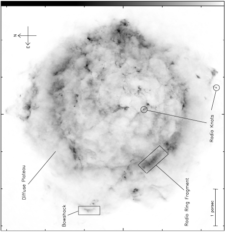
Figure 1: VLA image of Cas A at $\lambda\,$6.3 cm, showing examples of morphological classes of radio features referred to in the text. Axes (tangential projection in RA, DEC for epoch B1950) are annotated at intervals of 1 pc (60.7 arcsec for the distance of 3.4 kpc derived by Reed et al. reed (1995)), with the central (longer) tick indicating the B1950 centre of expansion of the system of fast optical filaments at RA 23:21:12.0 DEC +58:32:17.9 (Kamper & van den Bergh kamper (1976)). The greyscale spans the full dynamic range of 0.0 to 12.09 mJy per 0.375 arcsec pixel in 255 levels; a mild logarithmic scaling (0.85 exponent) has been applied to emphasise faint structures. The image was constructed from an almost fully sampled synthetic aperture using data from the VLA D, B, and A configurations at epochs 1983.0, 1984.0 and 1983.8, respectively (see table 1 of Braun et al. (braun (1987)) for observational parameters). The brightness distribution has been deconvolved from the synthesised point spread function using the maximum entropy method (AIPS task VM).

Perhaps the most straightforward suggestion, however, is that efficient electron acceleration occurs directly in regions of high radio brightness – in other words, that these regions are bright not only because of enhanced magnetic field, but also due to local enhancement of relativistic electrons. Such regions have been suggested to be sites of electron acceleration by a number of authors (e.g. Bell bell77 (1977), Dickel & Greisen dickel (1979), Cowsik & Sarkar cowsar84 (1984)). In Cas A they are represented by rather compact structures which include $\geq 300$ radio knots (Tuffs tuffs86 (1986), ARLPB) located in the shell, several paraboloidal radio features suggested to be bow shocks associated with decelerated ejecta (Braun et al. braun (1987)), and the bright fragmented radio ring at the projected radius of the (supposedly) reverse shock/contact discontinuity. Examples of all these morphological structures are depicted in Fig.1.

Any theory of particle acceleration in Cas A has to address a wide range of spatial and spectral characteristics of the observed nonthermal radiation from the radio to infrared (IR), and possibly to X-ray regimes, which can be summarized as follows:

• For $20\,{\rm MHz}\leq\nu\leq 30\,\rm GHz$ the total radio flux is well approximated by a power-law $J(\nu)\propto\nu^{-\alpha}$ with an index $\alpha\approx 0.77$ (e.g. Baars et al. baars (1977));

• For $\nu\leq 20\,\rm MHz$ the spectrum $J(\nu)$ essentially flattens, and turns over below 15 MHz (Baars et al. baars (1977));

• The secular decline of the fluxes seems to be frequency-dependent, with a decline rate at the level of $(0.8-1)\,\%/\rm yr$ in the frequency range $\nu\sim 40\,\rm MHz-1\,GHz$ (Rees rees (1990); Hook et al. 1992), and $\sim 0.6\,\rm\%/yr$ at $\nu\sim 10\,\rm GHz$ (Dent et al. dent (1974); O’Sullivan & Green osullivan (1999)).

• The contribution of the diffuse emission of the shell (plateau) to the total flux of Cas A at 5 GHz amounts to $\approx 50\,\%$, and the second half is due to the fragments of bright radio ring ($30\,\%$) and radio knots + bow shocks ($20\,\%$) (Tuffs tuffs86 (1986)). The total flux at the epoch 1987 was about 750 Jy (see ARLPB).

• Individual radio knots show a wide spread of spectral indices in the range from $\alpha\sim 0.6$ to $\alpha\sim(0.9-0.95)$ (Rosenberg rosenberg (1970); Tuffs tuffs83 (1983); ARLPB; AR96).

• For $\nu\geq 30\,\rm GHz$ the radio spectrum flattens to $\alpha\approx 0.65$ (Mezger et al. mezger (1986)) which possibly extends to the IR region if the flux of continuum emission measured at 6 $\mu\rm m$ by Tuffs et al. (tuffs97 (1997)) has a synchrotron origin.

• Recent observations reveal hard X-ray emission that extends with a power-law photon index $\alpha_{\rm x}\approx-3$ up to 120 keV (Allen et al. allen (1997); Favata et al. favata (1997)); a synchrotron origin of this radiation implies acceleration of electrons to multi-TeV energies.

Detailed studies based on high resolution mapping of Cas A at GHz frequencies have suggested that the identification of bright compact radio features with electron acceleration sites can be problematic (ARLPB; Anderson & Rudnick ar96 (1996), hereafter AR96). A particularly interesting finding of ARLPB and AR96 is a significant and rather unexpected correlation between the spectral index of the knots and their projected position in the shell, as well as their radio brightness: the steeper radio knots reside mostly in the outer regions of the shell, at $r\sim 2.5\,\rm pc$, and tend to be brighter.

The analysis in AR96 has shown that a self-consistent explanation of these correlations would be problematic if one assumes that the radio knots are the sites of efficient acceleration of the electrons. For an SNR as young as Cas A the radiative energy losses cannot modify the spectrum of radio electrons. Therefore in the framework of a ‘standard’ spatially homogeneous source model approach, one has to attribute the radio spectral indices observed to the source spectra of the electrons. The observed brightness/steepness trend of the radio knots would then apparently rule out effective electron acceleration in the knots, because such a process implies a hardening (see e.g. Berezhko & Völk berezhko (1997)), rather than a steepening of the particle spectra, typically to the power-law index $\beta\sim 2$.

There does exist however a natural way to modify the spectra of radio electrons, if we abandon the standard approach of a spatially uniform source for treatment of these electrons. Spectral modifications become unavoidable if we take into account energy-dependent propagation and escape of relativistic particles from the regions of higher concentration in an inhomogeneous medium. The efficiency of this process depends on the spatial gradients in the energy distribution $N({\bf r},E,t)$ of particles, and timescales of the spectral modifications can be as short as the escape time $\tau(E)$. This effect is widely used for the interpretation of the galactic CR spectra in the framework of diffusive or Leaky Box models, but it has not yet been given proper attention in studies of radio emission in the CR sources themselves.

In this paper we consider the consequensies of energy dependent propagation of relativistic electrons for the interpretation of the observed spectral, spatial and temporal characteristics of the broad-band nonthermal emission of Cas A. In Sect. 2 we introduce the ‘two-zone’ model for a spatially non-uniform radio source, separating compact regions with a high density of relativistic electrons (zone 1) from the rest of the shell where the electron density is significantly lower (zone 2). In Sect. 2 we consider in a qualitative way possible consequensies of such an approach for the interpretation of the observed radio data. In Sect. 3 we derive the system of kinetic equations for the electron energy distributions in the two zones. In Sect. 4 we assume that zone 1 components correspond to the sites of efficient electron acceleration, and show that this scenario is able to explain the broad band non-thermal radiation data of Cas A. In Sect. 5 we study the opposite scenario, which assumes that the enhancement of the electron density in zone 1 is caused not by active acceleration of particles there, but rather only by compression of the background population of relativistic electrons in the shell. We show that interpretation of the data within this latter scenario is problematic. In Sect. 6 we summarize the observational features which the model can explain, and in Sect. 7 we discuss implications and predictions of the model.

2 The model

2.1 Insufficiency of the single-zone approximation

To lowest approximation Cas A might be represented as a homogeneous shell containing magnetic field, relativistic electrons and gas. Although not reflecting the real pattern of the source, this ‘single-zone’ approximation allows estimates of basic parameters such as the mean magnetic field $B_{0}$ and energetics in radio electrons. In this approximation Cowsik & Sarkar (cowsar80 (1980)) have derived a lower limit to $B_{0}\geq 8\times 10^{-5}\,\rm G$, comparing the expected bremsstrahlung flux of GeV electrons with the upper limit $I(>100\,\rm MeV)\leq 1.1\times 10^{-6}\,\rm ph/cm^{2}s$ of SAS-2 (Fichtel et al. fichtel (1975)) and COS B detectors.

With the recent upper limits of the EGRET telescope, $I(>\!100\,\rm MeV)\leq 1.2\times 10^{-7}\,\rm ph/cm^{2}s$ (Esposito et al. esposito (1996)), this constraint on $B_{0}$ is significantly strengthened. In Fig. 2 we present the fluxes of the bremsstrahlung and synchrotron radiations calculated for 3 values of the mean magnetic field: $B_{0}=10^{-4}\,\rm G$, $\,3.5\times 10^{-4}\,\rm G$ and $7\times 10^{-4}\,\rm G$. For the mean gas density (in terms of ‘H-atoms’) we take $n_{\rm H}=15\,\rm cm^{-3}$, corresponding to $M\simeq 15\,M_{\odot}$ of matter in the shell (Fabian et al. fabian (1980), Jansen et al. jansen (1988), Reed et al. reed (1995)), and use a mean atomic $\overline{Z(Z+1)/A}=4.3$ derived by Cowsik & Sarkar (cowsar80 (1980)) from the elemental abundance estimates of Chevalier & Kirshner (chevkirsh (1978)) in Cas A. Continuous injection of electrons into the shell, with a spectrum $Q(E)\propto E^{-\beta_{0}}\,\exp(-E/E_{\rm c})$ where $\beta_{0}=2\,\alpha_{0}+1=2.54$ and an exponential cutoff energy $E_{\rm c}=100\,\rm TeV$, is assumed. The chosen $E_{\rm c}$ explains the fluxes of hard X-rays above 10 keV as synchrotron emission for the case of $B_{0}=10^{-4}\,\rm G$. However, this value of $B_{0}$ is unacceptable because the bremsstrahlung flux produced by GeV radio electrons is too high. The EGRET upper limit for the $\gamma$-ray flux of Cas A requires at least $B_{0}=3.5\times 10^{-4}\,\rm G$. Simultaneously we have to assume a significant flattening in the source spectrum of electrons below 100 MeV in order to avoid contradictions with the observed X-ray fluxes at 100 keV. For a single power-law distribution of electrons extending with $\beta_{0}=2.54$ down to the MeV region, the lower limit to the magnetic field is $B_{0}=7\times 10^{-4}\,\rm G$. Note however, that for $B_{0}\geq 3.5\times 10^{-4}\,\rm G$ the radiative energy losses of the electrons establish a spectral break at optical or lower frequencies, in which case the spatially homogeneous single-zone model fails to explain the observed hard X-ray fluxes by synchrotron radiation.

Figure 2: The fluxes of the synchrotron (heavy lines) and bremsstrahlung (thin lines) photons calculated in the framework of a spatially homogeneous single-zone model for the source function of accelerated electrons with power law index $\beta_{0}=2.54$ for 3 different values of the magnetic field: $B_{0}=10^{-4}\,\rm G$ (solid), $3.5\times 10^{-4}\,\rm G$ (dashed), and $7\times 10^{-4}\,\rm G$ (dot-dashed). The radio flux measurements shown correspond to the data from Baars et al. (baars (1977)) corrected for the secular decrease to the epoch 1986. The data at 1.3 mm (circle) and 1.2 mm (triangle) are from Chini et al. (chini (1984)) and Mezger et al. (mezger (1986)), respectively. The hatched region corresponds to the range of X-ray fluxes measured by Allen et al. (allen (1997)). Note that the RXTE fluxes are shown only above 10 keV since below 10 keV the X-ray fluxes are dominated by thermal emission. The OSSE measurements (The et al. the (1996)) are shown by crosses, and the bar corresponds to the EGRET upper limit above 100 MeV (Esposito et al. esposito (1996)).

2.2 The two-zone model

A more realistic model for Cas A has to account for the inhomogeneities in the radio brightness distribution and for the observed spread in the power-law exponents of the radio spectra of individual structures within $\alpha\simeq(0.6-0.9)$.

The simplest approximation for a non-uniform radio source corresponds to a ‘two-zone’ model, where the source with total volume $V_{0}$ consists of 2 different regions, or zones, with volumes $V_{1}$ and $V_{2}=V_{0}-V_{1}$, with 2 different spatial densities (concentrations) of radio electrons $n_{1}(E)=N_{1}(E)/V_{1}$ and $n_{2}(E)=N_{2}(E)/V_{2}$. Propagation effects may result in a significant difference between the two-zone and single-zone models only if these densities are essentially different. Therefore the principal definition for these two zones is that the concentration of electrons in zone 1 is much higher than in zone 2, $n_{1}\gg n_{2}$. The energy distributions of the electrons in these zones can be different. Therefore in the power-law approximation $N_{1,2}(E)\propto E^{-\beta_{1,2}}$ the exponents $\beta_{1}$ and $\beta_{2}$ can be different. Because the spectral ratio $n_{1}(E)/n_{2}(E)$ may thus depend on energy, it is convenient to specify that the condition $n_{1}\gg n_{2}$ relates first of all to electrons with energies $E\sim 1\,\rm GeV$ which are typically responsible for radio emission in the ‘1 GHz’ band.

In order to apply the two-zone model to Cas A, we have to foresee some observational manifestations of the radio emission of zones 1 and 2. It is reasonable to expect that not only the electron densities, but also the mean magnetic fields $B_{1}$ and $B_{2}$ in the two zones differ, with the magnetic field presumably being higher in the regions of higher electron densities. Therefore, the radio emissivities in these zones will be strongly contrasting, with regions belonging to zone 1 characterized by a much larger emissivity than regions in zone 2. It is also plausible that zone 1 components should be rather compact, with a small volume filling factor in the source, or otherwise the overall emission would be strongly dominated by this single zone.

Application of this criterion to Cas A immediately places all bright fragments of the radio ring in zone 1. Other constituents of zone 1 are the radio knots (and bow shocks) most of which are characterized by a strongly enhanced emissivity. We note however that in reality the knots embrace a wide range of emissivities, and because the simplified two-zone approach allows only 2 different electron densities (and emissivities), some compact structures with relatively low brightness should be more correctly classified as belonging to zone 2. This may have a physical basis – enhanced emissivity due to mild compression of magnetic fields, but without strong excess in the electon densities. Zone 2 then consists of the rest of the (spherical) shell between the radio ring and the outer edge of Cas A, i.e. the main body of the radio plateau, but also includes some low-brightness radio knots.

For purposes of practical classification of low-intensity knots it may prove useful to resort also to the second potentially observable distinction between zones 1 and 2 – different mean spectral indices $\alpha_{1}$ and $\alpha_{2}$ of their intrinsic emission. Due to a faster escape of higher energy electrons from the regions of high concentration, one could generally expect that the radiation spectra produced in zone 1 should be steeper, $\alpha_{1}>\alpha_{2}$ (see below Sect. 2.2.3). Because the spectral index of the total emission $\alpha_{0}\approx 0.77$ is to be maintained, an immediate conclusion is that the radiation spectrum of the diffuse zone 2 should be noticeably flatter, than the mean, i.e. $\alpha_{2}<\alpha_{0}<\alpha_{1}$.

Because of the complicated morphology, a quantitative treatment of the spectral indices of different types of structures is problematic in practice. In order to assess the characteristic values for $\alpha_{1,2}$, we note that the line of sight integrated radio brightness seen towards individual radio knots shows a broad range of spectral indices from $\alpha_{\rm min}\simeq 0.6$ to $\alpha_{\rm max}\simeq 0.95$, as measured by AR96 between $1.4\,\rm GHz$ and $5\,\rm GHz$. These spectral indices however do not always correspond directly to the intrinsic spectral indices of the knots, due to background contamination from the plateau. Although the detailed least square fitting procedure for spectral index measurements used in AR96 (their Sect. 2.4) largely removes this problem for knots with high contrast to the plateau, for faint knots at the limit of confusion with the plateau, the spectral index will be biased towards the (presumably flatter) index of that emission. In this regard, the result of AR96 presented in their Fig.6d appears as very informative. It shows that most of the radio knots found at large angular distances $\theta>130^{\prime\prime}$ (the projected $r_{\perp}=2.17\,\rm pc$) belong to the steep-spectrum population: from 62 such knots in total, 45 have indices $\alpha>0.8$, and 22 (i.e. $35\,\%$ !) belong to the ‘extreme’ end of the observed spectral indices $0.86<\alpha<0.95$. Because at these projected distances the brightness of the plateau is generally reduced, this may indicate that the intrinsic spectral index of the radio knots on average could be much steeper than the mean $\alpha_{0}$, and that the spectral index $\alpha>0.86$ of the ‘extremely steep’ population of the observed knots might be not so extreme, but rather a representative value for the intrinsic index of the knots. An (indirect) indication of this suggestion could be also another result shown in Fig. 6d of AR96: 83 from 123 knots found at angular distances close to the radio ring, $80^{\prime\prime}<\theta<120^{\prime\prime}$, where the brightness of the plateau is relatively high, belong to the population of knots with an ‘intermediate’ steepness $0.71\leq\alpha_{\rm obs}\leq 0.8$. As discussed below in Sect. 6, the model does not exclude a physical reason for such geometrical correlation between the knot index and its proximity to the ring. However, this effect can be explained also as a result of a line-of-sight mixture of comparable fluxes of the steep-spectrum knots with intrinsic $\alpha\sim(\alpha_{0}+0.1)$ and of the flat-spectrum diffuse plateau emission with $\alpha\sim(0.6-0.65)$ (see this Sect. below). Moreover, if we believe that the real geometry of the shell is quasi-spherical, it is difficult to suggest any other reasonable explanation, except for invoking the flux contamination effect, why only 2 knots from those 123 show the index $\alpha_{\rm obs}>0.83$, whereas the expected number of ‘extremely steep’ knots to be located at deprojected radii $r>2.17\,\rm pc$ but at the angular distances close to the “ring” should have been comparable with the number $22$.

We can conventionally define that all knots which have a moderate brightness and show spectral index $\alpha\leq 0.7$ belong to zone 2. Then, given the tendency for brighter knots to be steeper (AR96), this classification would retain most of the radio knots (at least in terms of their overal flux) in zone 1. At the same time, excluding thus the flat-spectrum knots from zone 1, for the average intrinsic spectral index of the remaining population of knots one can reasonably suppose $\alpha_{1,\rm kn}\sim(\alpha_{0}+0.1)=0.87$ or so.

It is possible that the intrinsic spectral index of the zone 1 components identified with the bright fragments of the radio ring is also close to this value. The low frequency measurements of Woan & Duffet-Smith (woan (1990); hereafter WDS90) at angular resolution $\geq 14^{\prime\prime}$ show that the average spectral index of the bright large radio components correlated with the ring is $\simeq 0.83$, i.e. again significantly larger than the mean $\alpha_{0}$ of the total emission. If we accept that the contribution of the diffuse emission, zone 2, may be flat, the intrinsic spectral index of the fragmented radio ring should be even larger. Then $\alpha_{1}\sim(\alpha_{0}+0.1)$ may be a reasonable value for the average spectral index of the entire zone 1. For qualitative discussions in this section we will use $\alpha_{1}=0.87$. We note however that our model does not pretend to predict characteristic spectral indices with the accuracy of the second digit after the comma.

The first zone will thus include a number $K\sim 200$ individual components, i.e. basically the bright fragmented radio ring, the ‘radio’ bow shocks, and the main part of all radio knots. Besides, zone 1 could also contain some regions of high concentration of electrons and high emissivities which are not immediately distinguished on the intensity maps either because of their very small sizes or because of strong contamination by, and confusion with the diffuse plateau emission. The latter may be the case if we believe that the fragmented “radio ring” actually represents a chain of large but geometrically flat (thin) structures of the “radio sphere” which are observed mostly ‘edge-on’. Then at angular distances interior to the ring, $\theta<80^{\prime\prime}$ or so, such fragments observed ‘face-on’ may easily merge with the plateau emission and show up as diffuse ‘clouds’ of only moderately enhanced brightness (see Fig. 1).

The flux produced in zone 1 can be estimated if we remember that at 5 GHz the (background subtracted) flux of the radio ring fragments makes up $\approx 30\%$, and that radio knots produce $\approx 20\%$ of the total flux (Tuffs tuffs86 (1986)). The latter value should be somewhat reduced for the flux of knots to be removed from zone 1 and classified in zone 2. On the other hand, it seems quite possible that up to $(5-10)\,\%$ of the total flux should be assigned to the ‘unseen’ population of zone 1 (especially, to face-on structures of the “radio sphere”). Therefore, we can estimate the overall flux $J_{1}$ of zone 1 as $\sim(45-55)\,\%$ of the total, concluding that the fluxes of zone 1 and zone 2 at 5 GHz are about the same, $J_{1}\simeq J_{2}$.

The spectral index $\alpha_{2}$ in the diffuse zone 2 can be then predicted if we note that the total flux has the form

$$J(\nu)=J_{1}\left(\frac{\nu}{5\,{\rm GHz}}\right)^{-\alpha_{1}}+J_{2}\left(\frac{\nu}{5\,{\rm GHz}}\right)^{-\alpha_{2}}\;.$$ (1)

In order for the mean spectral index between $\nu_{\ast}=1.4\,\rm GHz$ and $\nu_{\ast\ast}=5\,\rm GHz$ to be equal to $\alpha_{0}$, one needs a flux ratio

$$\frac{J_{2}}{J_{1}}=\frac{(\nu_{\ast\ast}/\nu_{\ast})^{\alpha_{1}-\alpha_{0}}-1}{1-(\nu_{\ast\ast}/\nu_{\ast})^{\alpha_{2}-\alpha_{0}}}\;\;\cdot$$ (2)

Then for $J_{2}=J_{1}$, $\alpha_{0}=0.77$, and $\alpha_{1}=0.87$, we find $\alpha_{2}=0.65$. It may somewhat vary assuming slightly different $J_{2}/J_{1}$ or $\alpha_{1}$ (or $\alpha_{0}$, which can be also slightly less than 0.77, see Fig.2). In particular, $\alpha_{2}$ may be rather close to 0.6 if we allow for the idea that the ‘unseen’ face-on structures of the “radio sphere” could contribute into zone 1 a third of what is contributed by the edge-on “radio ring”. Remarkably, these values of $\alpha_{2}$ correlate well with the lower range of spectral indices of the flat-spectrum radio knots. This suggests that flat-spectrum radio knots, with spectral indices close to 0.6 (or flatter than 0.7 as classified above) may indeed represent the regions of moderate local compression of the magnetic field and/or relativistic electrons of the diffuse shell, and therefore may give information about the spectrum of the background population of electrons there.

Thus, the model suggests a rather flat intrinsic spectrum of the radio plateau in the range $\alpha_{2}\simeq 0.6-0.65$, which corresponds to the spectral index of electrons $\beta_{2}\simeq 2.2-2.3$. For zone 1, $\alpha_{1}\simeq 0.87$ implies a rather steep electron spectrum with $\beta_{1}\simeq 2.74$. Taking into account the enhanced brightness of the compact zone 1, we will refer to zone 1 structures as the compact bright steep-spectrum radio (CBSR) components.

2.2.1 Synchrotron self-absorption in the two-zone model

Even though still highly simplified, this two-zone approach suggests a qualitative interpretation of several observed radio features of Cas A. In particular, it allows us to solve the problem of the low-frequency turnover below 20 MHz.

Although the measurements of KPDE at $\sim 100\,\rm MHz$ show evidence for thermally absorbing low-temperature gas in the central $\leq 1\,\rm pc$ region of Cas A, the thermal absorption cannot result in any noticeable effect in the shell where $T\sim 10^{7}\,\rm K$. On the other hand, in the case of a spatially homogeneous source (the shell) with a mean field $B_{0}=0.7\,\rm mG$, the process of synchrotron self-absorption results in a turnover of the radio spectrum only at frequencies below 5 MHz (see Fig.2). To explain the observed turnover below $20\,\rm MHz$, in a single-zone approach one needs $B_{0}\geq 5\,\rm mG$. But this assumption boosts the magnetic field energy up to $W_{\rm B}\geq 10^{51}\,\rm erg$, and therefore is hardly acceptable.

The situation essentially changes if one takes spatial inhomogeneities in the distribution of radio electrons and magnetic fields into account. Indeed, in the framework of the proposed two-zone approach the radio flux at frequencies well below 1 GHz is dominated by the steep-spectrum component, i.e. one has to require synchrotron self-absorption mainly of the zone 1 flux at $\nu<20\,\rm MHz$. Because of the very high density of the radio electrons and of the magnetic field in compact zone 1 components, synchrotron self-absorption there should be expected at frequencies significantly higher than in the single-zone model.

In order to estimate the model parameters needed for synchrotron self-absorption to occur below $20\,\rm MHz$, we note that for a power-law distribution of electrons $N(E)\propto E^{-\beta}$ the synchrotron luminosity can be expressed as

$$L(\nu) = 2\times 10^{-25}\,C_{\beta}\,N_{\ast}\,\left(\frac{B}{1\,\rm mG}\right)^{\frac{1+\beta}{2}}\times$$ (3)

$$\left(\frac{\nu}{10\,{\rm GHz}}\right)^{\frac{1-\beta}{2}}\;\;\rm\frac{erg}{s\,Hz}\;,$$

where $N_{\ast}\equiv\,E_{\ast}\,N(E_{\ast})$ with $E_{\ast}=1\,\rm GeV$. $C_{\beta}$ is a weak function of $\beta$ that changes within $1\pm 0.15$ for $\beta\sim(2-3)$, and we will assume $C_{\beta}=1$. With the same accuracy, the synchrotron absorption coefficient is given by

$$\kappa(\nu) \simeq 9\times 10^{-17}\,\beta\,10^{3\beta/2}\,\frac{N_{\ast}}{V}\,\left(\frac{B}{1\,\rm mG}\right)^{1+\beta/2}\times$$ (4)

$$\left(\frac{\nu}{10^{7}\,\rm Hz}\right)^{-(2+\beta/2)}\;\rm cm^{-1}\,,$$

where $V$ is the volume in units of $\rm cm^{3}$. The volume of zone 1 can be represented in the form $V_{1}=\sum_{i=1}^{K}V_{1}^{(i)}\simeq\overline{S}_{\rm pr}\bar{d}$, where $\bar{d}$ is the mean thickness of individual CBSR components along the line of sight and $\overline{S}_{\rm pr}=\sum_{i=1}^{K}\overline{s}_{i}$ is their overall surface in the plane of the sky. Requiring the synchrotron opacity to be significant at $\nu<20\,\rm MHz$ (which implies $\kappa\,\bar{d}\simeq 1$ at $\nu\simeq 15\,\rm MHz$) we obtain

$$\overline{S}_{\rm pr}\simeq 1.3\times 10^{37}\left(\frac{J_{1}}{400\,\rm Jy}\right)\,\left(\frac{B_{1}}{1\,\rm mG}\right)^{0.5}\;\rm cm^{2}\,.$$ (5)

For the external radius of the plateau region $R_{\rm 0}=2.5\,\rm pc$ this leads to an area filling factor

$$\frac{\overline{S}_{\rm pr}}{S_{0}}\simeq 0.07\,\left(\frac{J_{1}}{400\,\rm Jy}\right)\,\left(\frac{B_{1}}{1\,\rm mG}\right)^{0.5}\;,$$ (6)

where $S_{0}=\pi R_{0}^{2}$. For $B_{1}\simeq(1-2)\,\rm mG$ in zone 1 (see Sect. 4), the ratio $\overline{S}_{\rm pr}/S_{0}\sim 0.1$. From Fig.1 it is apparent that the area filling factor of all bright radio features is indeed of the order of 10 % .

From Eq.(5) it follows that the characteristic length scale for $K\sim 200$ CBSR components of the zone 1 should be of order $\Delta l\sim(\overline{S}_{\rm pr}/K)^{1/2}\sim 0.1\,\rm pc$. If we separate the radio knots from the larger fragments of the radio ring, and take into account that the flux $J_{\rm kn}$ of the knots constitutes about a third of $J_{1}$, the mean radius of the knots can be estimated as $\sim 0.03\,\rm pc$. At the distance 3.4 kpc this corresponds to the angular sizes of about $2^{\prime\prime}$, very similar to what is really observed.

2.2.2 Flattening of the radio spectrum

The superposition of flat and steep spectral components, with $J_{1}\simeq J_{2}$ around $5\,\rm GHz$, results in a flattening of the total radio spectrum at higher frequencies. Observations of Mezger et al. (mezger (1986)) do indicate a noticeable flattening of the Cas A spectrum in the wavelength range from $1\,\rm cm$ to 1mm, with power law index $\simeq\!0.65$ that possibly extends up to the near-IR region if the flux of continuum emission measured at $6\,\mu\rm m$ by Tuffs et al. (tuffs97 (1997)) is synchrotron in origin (see Fig.2).

Another important effect related to such composite fluxes consists in the possibility to give a new interpretation of the claimed secular flattening of the radio spectra (Dent et al. dent (1974); O’Sullivan & Green osullivan (1999)). Namely, the flattening of the radio spectra in time could be easily explained as being due to different rates of decline of the fluxes of the two zones, with the plateau emission dropping more slowly. Observations at 5 GHz have shown that the CBSR components are fading more rapidly than the total emission, which then requires that the plateau must be fading less rapidly (see Table 6.1 of Tuffs tuffs83 (1983)). If the plateau indeed were to have a flatter spectral index than the CBSR components, this would result in a flattening of the spectral index of Cas A with time. Note that previously, in the framework of the single-zone approach, the secular flattening could be explained only by the assumption of a gradual flattening of the spectrum of electrons either at higher energies or in time (Scott & Chevalier scott75 (1975), Chevalier et al. chevetal (1978), Cowsik & Sarkar cowsar84 (1984), Ellison & Reynolds ellison (1991)).

2.2.3 Effects of energy dependent propagation

Another advantage of a spatially inhomogeneous model is its ability to explain the basic characteristics of the observed nonthermal radiation in terms of very efficient acceleration processes operating in Cas A, which generally result in a source function of accelerated particles with hard spectral indices $\beta_{\rm acc}\simeq(2-2.2)$ (e.g. efficient Fermi acceleration at strong shock fronts). Even though the spectral index formally corresponding to the mean $\alpha_{0}=0.77$ is $\beta_{0}\geq 2.5$, the assumption of $\beta_{\rm acc}$ much harder than $\beta_{0}$ becomes possible if one takes into account the energy dependent propagation and escape of electrons from regions of high concentration on timescales $\tau_{\rm esc}(E)\propto E^{-\delta}$. For example, assuming that the sites of efficient particle acceleration are located in zone 1, one could expect that the electron energy distribution $N_{1}(E)$ formed there on timescales $t\gg\tau_{\rm esc}$ would have the power-law index $\beta_{1}=\beta_{\rm acc}+\delta$. On the other hand the leakage from zone 1 corresponds to injection of relativistic electrons into surrounding zone 2 with the rate $Q_{2}(E)=N_{1}/\tau_{\rm esc}\propto E^{-\beta_{2}}$ where $\beta_{2}=\beta_{1}-\delta=\beta_{\rm acc}\,$. With a reasonable source function index $\beta_{\rm acc}\simeq 2.2-2.3$ and energy-dependent escape with $\delta\sim 0.5$, the values of $\beta_{1}$ and $\beta_{2}$ needed for interpretation of the Cas A radio data could be reproduced.

Thus, the energy distribution of electrons $N_{1}(E)$ in the compact regions of efficient acceleration, which results in the enhanced density of relativistic electrons, may be actually much steeper than $N_{2}(E)$ in the surrounding volume. Interestingly, although the electron distribution $N_{2}(E)$ in the plateau region would show the hard spectral index of acceleration $\beta_{\rm acc}\,$, in principle no acceleration of electrons needs occur there at all. It is important to note, however, that on a qualitative level the same power-law indices $\beta_{2}$ and $\beta_{1}$ for both zones could be expected also in the case when relativistic electrons were accelerated in zone 2, while the electron density in CBSR structures would be enhanced due to local compression of the electrons, but not efficient acceleration in zone 1. To distinguish between these 2 basic scenarios, quantitative modelling is needed.

3 Kinetic equations in the two-zone model

Approximating the momentum distribution function of relativistic electrons as an isotropic function $f_{p}$ of the momentum $p=|\,{\bf p}\,|\,$, the kinetic equation for the energy distribution $f\equiv f({\bf r},E,t){\rm d}E=4\pi p^{2}f_{p}{\rm d}p$ of relativistic particles ($E\simeq pc$) can be written as:

$$\frac{\partial f}{\partial t} = {\rm div}_{\bf r}(D\,{\rm grad_{\bf r}}f)-{\rm div}_{\bf r}({\bf u}f)+\frac{{\rm div}_{\bf r}{\bf u}}{3}\frac{\partial}{\partial E}(Ef)$$ (7)

$$+\frac{\partial}{\partial E}(Pf)+A[f]\;.$$

Here ${\bf u}\equiv{\bf u}({\bf r},t)$ is the fluid velocity, $P\equiv P({\bf r},E,t)$ is the energy loss rate of electrons. Assuming isotropic diffusion, $D\equiv D({\bf r},E,t)$ is the scalar spatial diffusion coefficient, whereas $A[f]$ is a functional standing for various stochastic acceleration terms of electrons.

In the two-zone model the source with volume $V_{0}$ is subdivided into zone 1 composed of $K$ compact structures, with volume $V_{1}=\sum_{i=1}^{K}V_{1}^{(i)}\ll V_{0}$, spatially immersed in the zone 2 with $V_{2}=V_{0}-V_{1}\approx V_{0}$. The set of equations describing the evolution of the total energy distribution function of particles in these two zones, $N_{j}(E,t)={\int}f\,{\rm d}V_{j}\,$, can be found by integration of Eq.(7) over $V_{j}\,$ ($j=1,2$). Integration of the term $\partial f/\partial t$ over $V_{1}$ results in $\partial N_{1}/\partial t$. The volume integral of the two first terms in the right hand side of Eq.(7) is reduced to the sum of $K$ integrals on the surface $S_{1\,2}=\sum_{i}^{K}S_{i}$ separating the zone 1 components from zone 2:

$$\int_{V_{1}}[{\rm div}_{\bf r}(D\,{\rm grad_{\bf r}}f)-{\rm div}_{\bf r}({\bf u}f)]\,{\rm d}^{3}r =$$ (8)

$$\sum_{i=1}^{K}\;[\,\oint_{S_{i}}D\,({\bf e}\,{\rm grad}_{\bf r}f)\,{\rm d}s - \oint_{S_{i}}({\bf e\,u})f\,{\rm d}s\,]\;.$$

Here e is the unit vector perpendicular to the surface element ${\rm d}s$, directed outward from zone 1 to zone 2. These terms describe the rate of diffusive and convective exchange of particles between the two zones.

To proceed further, let us separate those parts of the interface $S_{1\,2}$ where the scalar product ($\bf u\,e$) has positive and negative signs: $S_{1\,2}=S_{+}+S_{-}$. The surface $S_{+}$ corresponds to the regions of plasma outflow from zone 1 into zone 2, so the integral over $S_{+}$ of the second term in Eq.(8) describes the convective escape of electrons, $-N_{1}(E,t)/\tau_{\rm c}$, where

$$\tau_{\rm c}\simeq\bar{h}/{u_{1}}\;,$$ (9)

$\bar{h}$ is characteristic thickness of, and $u_{1}$ is the plasma velocity in CBSR components.

The first integral in Eq.(8) over the surface $S_{+}$ can be simplified if we approximate $({\bf e}\,{\rm grad}f)\simeq(\bar{f}_{2}-\bar{f}_{1})/\Delta l\,$, where $\bar{f}_{1}\equiv\bar{f}_{1}(E,t)$ and $\bar{f}_{2}=\bar{f}_{2}(E,t)$ are the volume averaged distribution functions of relativistic particles in zones 1 and 2, respectively, and $\Delta l\equiv\Delta l(E,t)\,$ is the characteristic thickness of the transition layer between these zones. Taking into account that the volume of a body can be expressed as $V=ahS_{+}$, where $h$ is the thickness and $a\sim 1$ is a factor depending on the shape of the body, we find

$$\sum_{i=1}^{K}\oint_{S_{i+}}D\,({\bf e}\,{\rm grad}f) = \sum_{i=1}^{K}\frac{\bar{f}_{2}-\bar{f}_{1}}{\Delta l_{i}}\,\overline{D}_{i}\,S_{i+}$$ (10)

$$= \frac{\bar{f}_{2}-\bar{f}_{1}}{\tau_{\rm dif}}\,V_{1}\;,$$

where $\tau_{\rm dif}$ has the meaning of characteristic diffusive escape time of relativistic electrons from the regions of higher electron densities:

$$\frac{1}{\tau_{\rm dif}(E,t)}=\sum_{i=1}^{K}\frac{\overline{D}_{i}}{a{h}_{i}\Delta l_{i}}\,\frac{V_{1}^{(i)}}{V_{1}}\rightarrow\frac{\overline{D}_{\rm r}(E,t)}{a\bar{h}\Delta\bar{l}(E,t)}\;.$$ (11)

Here $\overline{D}_{\rm r}(E,t)$ corresponds to the mean of the spatial diffusion coefficient ${D}_{\rm r}({\bf r},E,t)$ on the surface $S_{+}$. Taking further into account that $N_{j}=V_{j}\,\bar{f}_{j}$  ($j=1,2$), the diffusive escape (exchange) term is reduced to the form

$$\frac{V_{1}\,N_{2}(E,t)}{V_{2}\,\tau_{\rm dif}(E,t)}-\frac{N_{1}(E,t)}{\tau_{\rm dif}(E,t)}\;\cdot$$ (12)

The integrals over the surface $S_{-}$ in Eq.(8) describe the inflow of electrons from zone 2, with some rate $Q_{2\,1}$, through the frontal surfaces of zone 1 components. For a mainly adiabatic compression of relativistic particles (see Sect. 5), $Q_{2\,1}$ could be directly connected with the energy distribution $N_{2}$ of electrons in zone 2. One could however expect the formation of strong shocks due to fast motion of CBSR components with respect to the surrounding plasma, so that the upstream electrons could be accelerated before entering zone 1. In that case $Q_{2\,1}$ would correspond to the source function of electrons accelerated on the shock fronts and injected into zone 1.

An essential part of the diffusive shock acceleration process is given by the adiabatic compression term in Eq.(7) (third term) in the shock region near the surface $S_{-}\,$. Therefore the volume integral of that term in a thin region adjacent to $S_{-}\,$ is to be formally incorporated into the source function $Q_{2\,1}$. The integral in the main part of the volume $V_{1}$ describes adiabatic energy losses (or gain) of electrons, and can be combined with the volume integral of the forth term in Eq.(7) as:

$$\frac{\partial}{\partial E}\int_{V_{1}}\left(E{\rm div}_{\bf r}{\bf u}/3+P\right)\,f\,{\rm d}^{3}r=\frac{\partial}{\partial E}\left(\,\overline{P}_{1}\,N_{1}\right)\;,$$ (13)

where $\overline{P}_{1}\equiv\overline{P}_{1}(E,t)$ is the mean rate of energy losses of electrons, which now includes also the adiabatic energy loss term $\overline{P}_{\rm ad}\simeq E\oint({\bf u\,e})\,{\rm d}s/3$.

Finally, the volume integral of the last term in Eq.(7) describes internal sources of accelerated electrons $Q_{1}^{\rm(int)}$ inside the volume $V_{1}$. The final equation then reads:

$$\frac{\partial N_{1}}{\partial t}=\frac{\partial(\,\overline{P}_{1}\,N_{1}\,)}{\partial E}\,-\,\frac{N_{1}}{\tau_{\rm esc}}\,+\,\frac{V_{1}\,N_{2}}{V_{2}\,\tau_{\rm dif}}\,+\,Q_{1}\;.$$ (14)

Here $Q_{1}\equiv Q_{1}(E,t)=Q_{2\,1}+Q_{1}^{\rm(int)}$ corresponds to the total injection rate of electrons in the first zone, and $\tau_{\rm esc}$ is the overall ”diffusive + convective” escape time of particles

$$\tau_{\rm esc}(E,t)=\left[\frac{1}{\tau_{\rm dif}(E,t)}+\frac{1}{\tau_{\rm c}(t)}\right]^{-1}\;.$$ (15)

Because $\tau_{\rm dif}$ generally increases for decreasing $E$, $\tau_{\rm esc}$ becomes energy independent at sufficiently small energies when $\tau_{\rm dif}\geq\tau_{\rm c}$. The range of actual energy dependence of $\tau_{\rm esc}$ is limited also at high energies since the diffusive escape time cannot be less than the light travel time across the CBSR components $\sim\bar{h}/c$. This obvious requirement formally follows from the condition that the characteristic lengthscale $\Delta\bar{l}(E)$ for spatial gradients in the distribution function $f({\bf r},E,t)$ cannot be less than the mean electron scattering path $\lambda_{\rm sc}(E)$, since otherwise the diffusion approximation implied in Eq.(7) fails. Taking into account that $D\sim\lambda_{\rm sc}c/3$, from Eq.(11) we find that indeed $\tau_{\rm dif}(E,t)\geq\tau_{\rm min}\simeq 3a\bar{h}/c$. Assuming $D(E)\propto E^{\,\delta_{1}}$, a reasonable approximation for the diffusive escape time is then

$$\tau_{\rm dif}(E,t)=\tau_{\ast}(t)\,(E/E_{\ast})^{-\delta}\,+\,\tau_{\rm min}(t)\;.$$ (16)

From Eq.(11) follows that generally the power-law index $\delta$ for diffusive escape time should be smaller than the index $\delta_{1}$ of the diffusion coefficient: since faster diffusion of more energetic particles tends to smooth out the gradients of the distribution function $f({\bf r},E,t)$ more effectively, the characteristic lengthscale $\Delta\bar{l}(E,t)$ should increase with energy. Then for a power-law approximation $\Delta\bar{l}\propto E^{\,\delta_{2}}$ the index $\delta_{2}>0$, so $\delta=\delta_{1}-\delta_{2}<\delta_{1}$. This conclusion is important since it allows us to assume a power-law index $\delta\sim 0.5-0.6$ needed for modification of the electron spectral index, not excluding at the same time efficient shock acceleration of particles in the Bohm diffusion limit which corresponds to $\delta_{1}=1$.

Integration of Eq.(7) over the volume of zone 2 results in an equation for $N_{2}(E,t)$:

$$\frac{\partial N_{2}}{\partial t}=\frac{\partial(\,\overline{P}_{2}\,N_{2}\,)}{\partial E}\,+\,\frac{N_{1}}{\tau_{\rm esc}}\,-\,\frac{V_{1}\,N_{2}}{V_{2}\,\tau_{\rm dif}}\,+\,Q_{2}\;,$$ (17)

where $\overline{P}_{2}$ is the mean energy loss rate, and $Q_{2}$ is the source function of electrons in zone 2. The second and third terms here result from the same surface integrals on the interface between zones 1 and 2 as in Eq.(8), but they have opposite signs since now the direction of the unit vector e is reversed. Note that formally the volume integrals in Eq.(8) result in two additional surface integrals describing particle exchange between zone 2 and the exterior on its outer boundary. However, this actually extends the two-zone model to a three-zone one, therefore we neglect here these exchange terms in order to remain in the framework of the two-zone approach.

The set of kinetic equations (14) and (17) describes the evolution of relativistic electrons in the general case of an expanding inhomogeneous source when the electron energy losses and particle exchange rates between two zones are time-dependent. Given these parameters and the source functions $Q_{1,2}(E,t)$, the electron energy distributions can be found numerically by iterations, using analytic solutions to the kinetic equation of electrons in an expanding homogeneous medium (Atoyan & Aharonian aa99 (1999)). To reduce the number of free parameters, we shall consider basically the case of a stationary source because the current energy distributions depend mostly on the injection of the electrons during recent (largest) timescales, $\Delta t_{0}\simeq 300\,\rm yr$. Only for calculations of the secular decrease of the fluxes we shall use the general results for an expanding source, taking into account adiabatic losses and decreasing average magnetic fields.

4 CBSR components as electron acceleration sites

Let us first consider the hypothesis that the compact bright radio components are the main sites of electron acceleration, and neglect possible acceleration in zone 2, i.e. $Q_{2}=0$. The electron injection function in zone 1 is approximated as

$$Q(E)=\,Q_{0}\,E^{-\beta_{\rm acc}}\exp(-E/E_{\rm cut})\;,$$ (18)

where we have omitted the suffix ‘1’ in $Q$. For calculations we assume equal radii $R_{\rm 1}$ and magnetic fields $B_{1}$ for zone 1 components.

Since the thickness $\bar{h}$ of a spherical object corresponds to its diameter, Eq. (9) gives $\tau_{\rm c}=2R_{1}/u_{1}$. For $R_{1}\sim(0.05-0.1)\,\rm pc$, and $u_{1}$ less than the sound speed $v_{\rm s}=\sqrt{\gamma_{\rm adb}kT/A\,m_{\rm p}}\sim 150\,\rm km/s$ in the gas with $T_{1}\leq 3\times 10^{7}\,\rm K$ and mean atomic $A\sim 15$ (corresponding to $\overline{Z(Z+1)/A}\simeq 4.3$, Cowsik & Sarkar cowsar80 (1980)), the time $\tau_{\rm c}$ is larger than the source age $t_{0}\simeq 300\,\rm yr$. Therefore the precise value of $u_{1}$ will not significantly affect the results. The minimum escape time of electrons from the zone 1 is taken as $\tau_{\rm min}=R_{1}/c$.

Figure 3: The energy distributions of the electrons in zone 1 (solid) and zone 2 (dashed), calculated in the two-zone model assuming that the CBSR components in CAS A correspond to the sites of electron acceleration. The dot-dashed curve corresponds to the initial iteration for the energy distribution of electrons in zone 1 when the ‘return’ diffusive flux of electrons from zone 2 into zone 1 is neglected (the term $\propto N_{2}/\tau_{\rm dif}$ in Eq.14). Parameters for the source function are $\beta_{\rm acc}=2.24$, $E_{\rm c}=3.5\times 10^{13}\,\rm eV$; the magnetic fields $B_{1}=1.5\times 10^{-3}\,\rm G$ and $B_{2}=4\times 10^{-4}\,\rm G$; the diffusive escape time is defined by $\tau_{\ast}=25\,\rm yr$ and $\delta=0.6$. For zone 1, $K=200$ components with the radius $R_{1}=0.05\,\rm pc$ are supposed.

The time $\tau_{\ast}$ in Eq.(1) defines the ratio of the magnetic fields in two zones needed for an explanation of the flux ratio $J_{1}/J_{2}\simeq 1$. Indeed an effective modification of the injection spectrum of radio electrons in the GeV region implies that at these energies the overall escape time $\tau_{\rm esc}(E)\simeq\tau_{\ast}(E/E_{\ast})^{\delta}$, and that it is significantly smaller than $t_{0}\simeq 300\,\rm yr$. The leakage of the electrons from $V_{1}$ will result in $N_{2}(E)\sim N_{1}(E)\,t_{0}/\tau_{\rm esc}(E)$ electrons accumulated in the surrounding zone 2. Using also Eq.(3), we then find

$$\frac{B_{1}}{B_{2}}\simeq\left(\frac{t_{0}}{\tau_{\ast}}\right)^{\frac{2}{1+\beta_{2}}}\left(\frac{2\,B_{1}}{1\,{\rm mG}}\right)^{\frac{\beta_{2}-\beta_{1}}{1+\beta_{2}}}\left(\frac{J_{1}}{J_{2}}\right)^{\frac{2}{1+\beta_{2}}}\;,$$ (19)

Thus, for $\tau_{\ast}\leq 0.1\,t_{0}$ the ratio $B_{1}/B_{2}\geq 3$.

In Fig.3 we show the energy distributions of electrons $n_{1,2}(E)=N_{1,2}(E,t_{0})/V_{1,2}$ calculated the injection spectrum with $\beta_{\rm acc}=2.24$ and $E_{\rm c}=35\,\rm TeV$, and the escape time parameters $\tau_{\ast}=25\,\rm yr$ and $\delta=0.6$. At GeV energies the power law index of electrons in zone 1 is indeed strongly modified, almost reaching the maximum theoretical value $\beta_{1}\approx\beta_{\rm acc}+\delta$. However both at lower and higher energies there is some flattening of $n_{1}(E)$. At energies $E\leq 100\,\rm MeV$ the flattening is connected with the increase of the escape time to $\tau_{\rm dif}>100\,\rm yr$, which becomes comparable to the age of Cas A, reducing thus the efficiency of the ecape. At high energies $\tau_{\rm dif}(E)$ is limited by the energy-independent minimum escape time $\tau_{\rm min}$ in Eq.(16). This effect can be seen in Fig.3 for the dot-dashed curve at $E\geq 100\,\rm GeV$. Note, however, that for the self-consistently calculated spectrum (solid curve) of electrons in zone 1 the flattening is noticeable already at energies $E\geq 10\,\rm GeV$ where $n_{1}(E)$ becomes comparable to $n_{2}(E)$. At these energies the gradients in the spatial distribution of relativistic electrons in the source become small, reducing the net exchange of particles between the zones, which again results in a less efficient modification of $Q(E)$.

Figure 4: The fluxes of synchrotron (heavy lines) and bremsstrahlung (thin lines) photons produced by electrons shown in Fig.3. The dashed and dot-dashed curves correspond to the fluxes expected from the compact radio structures and the diffuse plateau, respectively, and the solid curves correspond to the synchrotron and bremsstrahlung fluxes of two zones. The full dots show the total nonthermal flux.

Figure 5: The spectral indices of the synchrotron fluxes corresponding to the total (solid), zone 1 (dashed), and zone 2 (dot-dashed) radiations shown in Fig.4

The synchrotron and bremsstrahlung fluxes are presented in Fig. 4, and Fig. 5 shows the spectral indices at different frequencies. Because the synchrotron radiation in zone 1 is steep, it becomes dominant at low frequencies. The compactness of zone 1 components leads to synchrotron self absorption at $\nu\leq 20\,\rm MHz$. At frequencies above 5 GHz the plateau emission dominates resulting in a noticeable flattening of the overall spectrum in the far infrared (FIR). All these results are in agreement with expectations derived qualitatively in Sect. 2.

For the model parameters used in Fig.4 the energy content in relativistic electrons in zones 1 and 2 is $W_{\rm e1}=1.3\times 10^{48}\,\rm erg\,$ and $\,W_{\rm e2}=1.4\times 10^{48}\,\rm erg$, respectively, and the energy in the magnetic fields $W_{\rm B1}=2.6\times 10^{47}\,\rm erg$ and $W_{\rm B2}=6.8\times 10^{48}\,\rm erg$. The total energy in relativistic electrons, $W_{\rm e}=W_{\rm e1}+W_{\rm e2}$, can be estimated analytically taking into account that: (a) the shape of the overall energy distribution of electrons $N(E)=N_{1}(E)+N_{2}(E)$ repeats the power law injection $\propto E^{-\beta_{\rm acc}}$ until the break energy $\sim\!300\,\rm GeV$ due to synchrotron losses (in zone 2), and (b) the total number of GeV electrons $N_{\ast}=E_{\ast}\,N(E_{\ast})$ (with $E_{\ast}=1\,{\rm GeV}\approx 2000\,m_{\rm e}c^{2}$) is defined mainly by electrons in zone 2, $N_{\ast}\approx N_{\ast 2}$, which can be estimated using Eq.(3). For $\beta_{\rm acc}\geq 2.1$ we find

$$W_{\rm e}\approx\,2.2\times 10^{46}\;\frac{(2000)^{\beta_{\rm acc}-2}}{\beta_{\rm acc}-2}\left(\frac{B_{2}}{1\,\rm mG}\right)^{-\frac{\beta_{\rm acc}+1}{2}}\;\rm erg\;.$$ (20)

For $\beta_{\rm acc}=2.24$ and $B_{2}=0.4\,\rm mG$ this equation results in $W_{\rm e}\approx 2.5\times 10^{48}\,\rm erg$, in agreement with the numerical results.

Figure 6: Radiation fluxes calculated for $\beta_{\rm acc}=2.2$ and 3 different magnetic fields $B_{1}$ in zone 1, $B_{1}=1\,\rm mG$ (solid), 1.6 mG (dashed), and 3 mG (dot-dashed), assuming the same ratio $B_{1}/B_{2}=4$. Exponential cutoff energies $E_{\rm c}$ and escape times $\tau_{\ast}$ in these 3 cases are: $E_{\rm c}=16\,\rm TeV$ and $\tau_{\ast}=26\,\rm yr$ (solid), $E_{\rm c}=27\,\rm TeV$ and $\tau_{\ast}=20\,\rm yr$ (dashed), and $E_{\rm c}=200\,\rm TeV$ and $\tau_{\ast}=14\,\rm yr$ (dot-dashed). For the assumed here number of zone 1 components $K=150$ with radius $R_{1}=0.06\,\rm pc$ the sky covering fraction of the zone 1 is 0.09 .

In Fig.6 we show the fluxes calculated for $\beta_{\rm acc}=2.2$ and different values of the magnetic fields in zones 1 and 2. For all 3 cases the spectra of synchrotron radiation coincide up to the IR, but at higher frequencies they differ because of radiative break induced by synchrotron losses. Note that for interpretation of the X-ray fluxes above 10 keV one needs higher values of the exponential cutoff energy for higher magnetic field $B_{1}$: $E_{\rm c}=16\,\rm TeV$ for $B_{1}=1\,\rm mG$ and $E_{\rm c}=27\,\rm TeV$ for $B_{1}=1.6\,\rm mG$. For $B_{1}=3\,\rm mG$ the calculated synchrotron fluxes remain significantly below the observational data even assuming $E_{\rm c}=200\,\rm TeV$.

However, the synchrotron losses in high magnetic fields effectively limit the maximum energy of electrons to values well below $E_{\rm c}\simeq 200\,\rm TeV$. For example, in the case of diffusive shock acceleration, the acceleration rate can be estimated as ${\rm d}E/{\rm d}t\sim Eu_{2}^{2}/D(E)$, where $D(E)$ is the diffusion coefficient and $u_{2}$ is the speed of CBSR components with respect to the surrounding plasma. Equating this rate in the Bohm diffusion limit to the synchrotron loss rate, the characteristic maximum energy of electrons can be estimated as:

$$E_{\rm c}^{\rm(max)}\simeq 3\times 10^{13}\left(\frac{u_{2}}{3000\,\rm km/s}\right)\left(\frac{B}{1\,\rm mG}\right)^{-1/2}\,\rm eV.$$ (21)

Comparison with the values of $E_{\rm c}$ in Fig. 6 shows that diffusive shock acceleration could be consistent with synchrotron origin of the hard X-rays from Cas A for $B_{1}<2\,\rm mG$. Higher values of $B_{1}$ would require a more efficient acceleration mechanism. But anyway, the value of $B_{1}=3\,\rm mG$ is a very conservative upper limit of our model for the mean magnetic field in the bright radio structures if the measured hard X-ray flux has synchrotron origin. At the same time, the lower limit for $B_{1}$ is about 1 mG, which is needed for consistency of the bremsstrahlung with the flux upper limits of EGRET and OSSE detectors (see Fig.6). It is interesting that magnetic fields corresponding to the energy equipartition with relativistic electrons in the CBSR components are in the range $B_{1}\simeq(1.5-2)\,\rm mG$.

Another feature to be addressed in this section is the wavelength-dependent rate $-{\rm d}\ln J(\nu)/{\rm d}t$ of the secular decline of radio fluxes. For calculations of this rate we need to specify the rates of the magnetic field decline and the adiabatic losses of electrons. For a spherical source (shell) homogeneously expanding with speed $u_{0}$, the adiabatic losses $P_{\rm ad}=E/t_{\rm ad2}\,$, where $t_{\rm ad2}\simeq t_{\rm exp}=R_{0}/u_{0}\simeq 1000\,\rm yr$ corresponds to the current expansion time (‘age’) of the outer shell. In the ‘standard’ power-law approximation for the magnetic field declining with the shell radius as $B(R_{0})\propto R_{0}^{-m}$, the characteristic decline time $t_{\rm B}=B/(-{\rm d}B/{\rm d}t)=t_{\rm exp}/m$. For a magnetic field ‘frozen’ into the spherically expanding source $m=2$, but $m<2$ if the fields are effectively created in the shell. The assumption $m\simeq 1.5$ results in $t_{\rm B2}\simeq 700\,\rm yr$. Concerning zone 1, we note that along with the compact radio structures with declining brightness observations show also a large number of brightening components, and the timescales of the flux variations in the individual knots can be as small as few tens of years (Tuffs tuffs86 (1986), AR96). An estimate of the average time $t_{\rm B1}$ of the magnetic field decrease in CBSR components is thus problematic. Therefore we consider $t_{\rm B1}$ as a free model parameter, and neglect adiabatic losses of electrons there (if any – especially as they are supposed to be the sites of effective acceleration).

Figure 7: The rate of secular decline of the total flux of synchrotron radiation shown in Fig.4, calculated for characteristic timescales (see text) $t_{\rm B2}=650\,\rm yr$ and $t_{\rm ad2}=1000\,\rm yr$ for zone 2, and different timescales for the magnetic field decline in zone 1: $t_{\rm B1}=115\,\rm yr$ (dot-dashed), 130 yr (solid), 150 yr (dashed). The diamond shows the recent result of O’Sullivan & Green (osullivan (1999)) at 15 GHz, all other data points are from Rees (rees (1990)). The heavy dashed straight line corresponds to the earlier ‘best fit’ estimate (see text).

Calculations of the secular decline rate of the fluxes at different frequencies are presented in Fig. 7. The straight heavy dashed line shown corresponds to the decline rate deduced by Dent et al. (dent (1974)) and Baars et al. (baars (1977)) from comparison of the decline rate $\simeq 1.29\,\%/\rm yr$ measured then at 81 MHz by Scott et al. (scott69 (1969)) with the data in the 1-10 GHz region. Later measurements have shown that the decline rate around $\nu\sim 100\,\rm MHz$ is at the same level $\sim(0.8-1)\,\%/\rm yr$ as at $\nu\sim 1\,\rm GHz$, which has placed doubt on the frequency dependence of the decline rate in general (Rees rees (1990); Hook et al. hook (1992)). However, the recent result of O’Sullivan & Green (osullivan (1999)) that the flux decline rate at 15 GHz is about $0.6\%/\,\rm yr$, seems to confirm the effect of slower decline of radio fluxes at high frequencies.

Figure 7 shows that practically all the observational data can be well explained assuming the average magnetic field decline time in zone 1 of order $t_{\rm B\,1}\sim 120-150\,\rm yr$. Note that a significant drop of the secular decline rate predicted at $\nu<30\,\rm MHz$ is connected with the gradual decrease of synchrotron self-absorption in zone 1.

5 CBSR components as acceleration-passive sites

Consider now the hypothesis that acceleration of electrons takes place only in zone 2 and is negligible in zone 1. In this case the source function $Q_{2}(E)$ for zone 2 is in the form of Eq.(18), while $Q_{1}(E)$ for zone 1 is defined only by the rate $Q_{2\,1}(E)$ of advection of relativistic electrons from the plateau region. The required for zone 1 relativistic electron density enhancement could be then supposed as being due to adiabatic compression of the zone 2 electrons on the front surface $S_{-}$ of fastly moving CBSR components, and their subsequent accumulation in zone 1 over timescales $\Delta t\sim\tau_{\rm esc}$. Neglecting in Eq.(7) the diffusion term on the surface $S_{-}$, in compliance with the assumption of negligible diffusive acceleration there, and retaining only the convection and the adiabatic compression terms, the equation describing the transport of the electrons through $S_{-}$ reads:

$$u_{x}\frac{\partial f_{p}}{\partial x}-\frac{\partial u_{x}}{\partial x}\,\frac{p}{3}\frac{\partial f_{p}}{\partial p}=0\;,$$ (22)

where $f_{p}\equiv f_{p}(x,p,t)$ is the momentum distribution function, $x$ is the spatial coordinate and $u_{x}$ is the plasma speed along the $x$-axis perpendicular to the compression layer. General solution to this equation reads: $f_{p}(p,x)=F_{0}[p(u_{x}/u_{0})^{1/3}]$, where $F_{0}(p)=f_{p}(p,x_{0})$ is an arbitrary initial function. Connecting the electron distribution functions across the layer, the injection rate of relativistic electrons from zone 2 into zone 1 is found:

$$Q_{2\,1}(E)\simeq N_{2}(E\,\rho_{\rm c}^{-1/3})\,\rho_{\rm c}^{-1/3}\,S_{-}\,u_{2}\,V_{2}^{-1}\;,$$ (23)

where $\rho_{\rm c}=u_{2}/u_{1}$ is the mean compression ratio, and $u_{2}$ and $u_{1}$ correspond to the plasma speeds of the plasma in the upstream and downstream regions in the rest frame of the CBSR components.

Considering possible values of $u_{2}$, note that for the mean radial expansion age of radio knots $t_{\rm exp}=r/v_{\rm r}$ within $(550-1000)\,\rm yr$ (Tuffs tuffs86 (1986); Anderson & Rudnick ar95 (1995)) the characteristic speed of the knots may be estimated as $v_{\rm kn}\simeq(1700-3200)\,\rm km/s$. Taking into account that surrounding plasma in the shell is moving in the same direction, and as evidenced by a shorter X-ray expansion time scales $\sim 600\,\rm yr$ (Koralesky et al. koralesky (1998); Vink et al. vink (1998)), appears to be overtaking most of the compact radio knots, the value $u_{2}\sim 2000\,\rm km/s\,$ seems a reasonable estimate for the relative speed of radio knots with respect to the surrounding medium. For the bright radio ring $t_{\rm exp}\simeq 950\,\rm yr$ (Tuffs tuffs86 (1986)), corresponding to $v_{\rm ring}\simeq 1700\,\rm km/s$, while the speed of freely expanding ejecta upstream of the reverse shock, i.e. at $r<R_{\rm ring}$, is about $(5000-5300)\,\rm km/s$. Thus, for the radio ring $u_{2}\sim 3500\,\rm km/s\,$, and we can take $3000\,\rm km/s\,$ as a reasonable maximum value of $u_{2}$ for the zone 1.

The compression ratio $\rho_{\rm c}$ can be approximated as the ratio of magnetic fields $\rho_{\rm c}\simeq B_{1}/B_{2}$. The energy distributions of the radio electrons can be connected as

$$\frac{N_{1}(E_{\ast})}{N_{2}(E_{\ast})}\simeq\frac{V_{1}}{V_{2}}\,\left(\frac{B_{1}}{B_{2}}\right)^{\frac{\beta_{2}-1}{3}}\frac{u_{2}\,\tau_{\ast}}{2\,R_{1}}\;,$$ (24)

using the relation $N_{1}(E_{\ast})\simeq Q_{2\,1}\times\tau_{\ast}$. Eqs. (3) and (24) result in

$$\left(\frac{B_{1}}{B_{2}}\right)^{\frac{5\,\beta_{2}+1}{6}}\simeq\,\frac{J_{1}}{J_{2}}\,\frac{2\,R_{1}\,V_{2}}{u_{2}\,\tau_{\ast}\,V_{1}}\,\left(\frac{2\,B_{1}}{1\rm mG}\right)^{\frac{-\Delta\beta}{2}}\;,$$ (25)

where $\Delta\beta=\beta_{1}-\beta_{2}$. Since the volume filling factor of the compact zone 1 structures is $V_{1}/V_{2}\sim 0.5\,\%$ or less, and since for effective modification of the electron spectra by escape one needs $\tau_{\ast}\leq 0.1\,t_{0}=30\,\rm yr$, the ratio of the magnetic fields in the two zones should be rather high, $B_{1}/B_{2}>10$.

The results of numerical calculations are shown in Fig.8. The total flux seems to fit the data practically equally well as in Fig. 4 earlier. However, a closer look to these figures reveals significant differences. First of all, in Fig. 8 the agreement with the radio data is reached due to a much higher contribution of zone 1 to the overall flux. In particular, at 5 GHz the partition of the fluxes corresponds to $J_{1}/J_{2}\simeq 3$, instead of $J_{1}/J_{2}\simeq 1$. Secondly, although here we have assumed high $\delta=0.75$, the calculations show that the spectral index of the electrons swept up from zone 2, $\beta_{2}=2.2$, was steepened in zone 1 only to values $\beta_{1}\leq 2.6$, well below the ‘expected’ value 2.95. Obviously, this is far insufficient for explanation of the observed steep spectral indices of the radio knots.

Figure 8: Radiation fluxes expected in the scenario when acceleration occurs only in the zone 2 (diffuse plateau), but not in the compact zone 1. The solid lines show the total fluxes, while the dashed and dot-dashed lines correspond to the contributions from the zone 1 and zone 2, respectively. Model parameters are: $B_{1}=3.8\,\rm mG$, $B_{2}=0.2\,\rm mG$ $\beta_{\rm acc}=2.2$, $E_{\rm c}=30,\rm TeV$, $\tau_{\rm ast}=20\,\rm yr$, $\delta=0.7$, $K=200$, $R_{1}=0.06\,\rm pc$, and $u_{2}=3000\,\rm km/s$.

Figure 9: The energy distributions of the electrons formed in zone 1 (solid line) and zone 2 (dashed line) in the framework of ‘adiabatic compression’ scenario for zone 1 electrons, calculated for parameters in Fig.8. The dot-dashed curve corresponds to the the energy distribution of electrons in zone 1 when the return diffusive flux of electrons from zone 2 into zone 1 is neglected.

The reason for difficulties arising in the scenario that assumes only passive compression, but not active acceleration of electrons in zone 1, can be understood from Fig. 9 where we show the spatial densities $n_{1,2}(E)$ of the electrons in zones 1 and 2. The dot-dashed line shows the spectrum of the electrons which would be formed in the zone 1 if one neglects the term $\propto n_{2}/\tau_{\rm dif}$ in Eq.(14). This spectrum is steep. But when the effect of spatial density gradients between the two zones is taken into account correctly, the situation dramatically changes. The energy dependent propagation can result in a significant steepening of the source spectra only in the regions of higher spatial densities of relativistic particles. Otherwise diffusive exchange of particles tends to equalize $n_{1}(E)$ with $n_{2}(E)$ resulting in $\beta_{1}\rightarrow\beta_{2}$ independently of $\delta$, until the radiative losses become important.

Thus, for an effective modifications of the initial source spectrum of the radio electrons the condition $n_{1}(E)\gg n_{2}(E)$ should be satisfied. The ratio of electron densities expected at 1 GeV can be estimated from Eqs. (25) and (26) (assuming $\beta_{2}\simeq 2.2$) as:

$$\frac{n_{\ast 1}}{n_{\ast 2}}\simeq\left(\frac{J_{1}}{J_{2}}\right)^{0.2}\left(\frac{V_{2}}{V_{1}}\right)^{0.2}\left(\frac{u_{2}\,\tau_{\ast}}{2\,R_{1}}\right)^{0.8}\left(\frac{2\,B_{1}}{1\rm mG}\right)^{-0.1\,\Delta\beta}.$$ (26)

For the parameters used in Fig.8 this equation predicts $n_{\ast 1}/n_{\ast 2}\approx 2$, in agreement with numerical calculations, which is smaller by a factor of $15$ than similar ratio in Fig.3. Calculations show that it is not easy to increase this ratio significantly, remaining within the ‘adiabatic compression’ scenario.

Thus, a self-consistent explanation of the observed radio fluxes of Cas A is very problematic, unless we assume an effective acceleration of electrons in the CBSR components in order to build up sizeable gradients in the spatial distribution of the radio electrons in the source.

6 Results

The spatially non-uniform source model, even in its simplest two-zone form, allows us to unify into a single picture many observational data on the broad-band nonthermal radiation of Cas A. The following is the summary of observational features of Cas A which could be explained in the framework of this model.

The brighter radio structures tend to be steeper (AR96) to the extent that the energy density of relativistic electrons there would be higher. In principle, even assuming the same hard power law index for the acceleration, e.g $\beta_{\rm acc}\simeq 2.2$, and $\delta\simeq 0.6$ for the escape of the electrons, it is possible to explain the observed variations of the spectral indices of individual compact radio structures from $\alpha_{2}\sim 0.6$ to $\alpha_{1}\sim 0.9$. Such variations can be connected with two effects.

(a)   The intrinsic index of some knots will be flatter than the maximum possible $\alpha_{1}=\alpha_{2}+\delta/2$ if the local gradient $n_{1}/n_{2}$ is not sufficiently high, and if the characteristic escape time $\tau_{\ast}$ of GeV electrons from these knots is larger than $\sim 30\,\rm yr$. The impact of the latter effect can be seen in Figs. 10 and 11, where we show the fluxes and spectral indices calculated in the modified two-zone model approach, subdividing the CBSR structures in two groups and assuming 2 different spatial/temporal scales for larger (‘ring’) and smaller (‘knot’) components in zone 1.

Figure 10: Fluxes expected in the framework of the modified two zone model, when in zone 1 more compact radio knots (dashed line) and larger fragments of the radio ring (thin solid line) are separated. The 3-dot–dashed line shows the total flux from zone 1, and the dot-dashed line shows the flux from zone 2. The total synchrotron flux is shown by the heavy solid line. The model parameters are the following. For the knots: $R_{\rm 1.kn}=0.033\,\rm pc$, $\tau_{\ast}=15\,\rm yr$, $\delta=0.6$, $K_{\rm kn}=180$; for the ring fragments $R_{\rm 1.ring}=0.1\,\rm pc$, $\tau_{\ast}=35\,\rm yr$, $\delta=0.6$, $K_{\rm ring}=20$. The same $\beta_{\rm acc}=2.2$ and cutoff energy $E_{\rm c}=35\,\rm TeV$ for the accelerated electrons, and magnetic fields $B_{1.\rm kn}=B_{\rm 1.ring}=1.5\,\rm mG$ in the knots and the ring is assumed. The magnetic field $B_{2}=0.36\,\rm mG$.

Figure 11: The spectral indices of the radiation components shown in Fig.10

(b)  The intrinsic spectrum of individual knots could be steep, up to $\alpha_{1}\simeq 0.9$, but the observed spectrum may be flatter, depending on the degree of flux contamination by the flat-spectrum radiation from the diffuse plateau along the line of sight to the knot. This effect may be relevant mainly to those cases when the background subtraction is problematic (e.g., for the structures with insufficiently high contrast to the plateau).

The strong correlation between the spectral index and the projected position of radio knots observed by AR96 could be connected with both effects (a) and (b). Indeed, the brightness of the diffuse plateau seems to decrease from the radio ring towards the outer edge of the shell more rapidly than one would expect merely on the base of the projection effect in a spherical geometry (see Fig.7 from ARLPB). This implies that the density $n_{2}$ of radio electrons could be higher at distances closer to the ring. Then the steepest knots would be found predominantly closer to the edge of the plateau, because (i) the local ratio $n_{1}/n_{2}$ might be higher far from the reverse shock, and (ii) contribution of the flat spectrum plateau emission to the steep spectrum flux of the knots is smaller in directions to the projected periphery of the shell.

The cutoff of the radio spectrum below 20 MHz is explained by the synchrotron self-absorption of the flux of zone 1. This interpretation is possible basically because the model predicts that the intrinsic fluxes of the compact bright structures are much steeper than the spectra in the diffuse plateau. Then at low frequencies the flux of CBSR components should dominate the total radio emission. Therefore synchrotron self-absorption of only this flux, which becomes possible due to high density of particles (and fields) in those compact structures, is sufficient to comply with the data.

It is worth noticing that due to variations of the physical parameters in the individual CBSR components contributing to zone 1 flux, one could generally expect that the synchrotron absorption of that flux would be in reality smoother than it is shown in Fig. 4 where we have assumed the same parameters for all counterparts of zone 1. The position of the characteristic cutoff frequency for an individual component $j$ is found from the condition $\tau_{j}(\nu)=1$ where $\tau_{j}=R_{j}\kappa(\nu)$ is its opacity. From Eqs. (3) and (4) it follows that $\tau_{j}(\nu)\propto A_{j}\nu^{-(2+\beta_{j}/2)}$, with $A_{j}=R_{j}^{-2}f_{j}B_{j}^{0.5}$ where $f_{j}$ is the knot flux (luminosity) at some fixed frequency (say 1 GHz). Because of the very strong dependence of $\tau_{j}$ on $\nu$, a significant broadening of the synchrotron turnover frequency for the ensemble of CBSR components (say by a factor 2) would be expected only if the luminosity-weighted dispersion $\sigma$ of the parameter $A_{j}$ is very large ($\sigma\simeq 10$). The fact that the observed turnover is sharp may then imply a quite reasonable possibility – that the distribution of the parameters $\{A_{j}\}$ is not far from ‘Gaussian noise’. In that case one would normally expect $\sigma\sim 1$ (or perhaps even less, given the expected correlation of $f_{j}$ and $R_{j}$), so the synchrotron turnover position would be effectively dispersed, or broadened, only by a factor roughly $(1+\sigma)^{0.3}\simeq 1.2$, i.e. about $\pm 20\%$ around the mean position. Note that the overall flux in Fig.10, where 2 significantly different sizes for the large and small components are assumed, show practically the same sharp cutoff below 20 MHz as in Fig.4.

Observations at low frequencies by KPDE, at a resolution of about $20^{\prime\prime}$, show that the spectral index of Cas A between 333 MHz and 1.38 GHz is approximately constant, $\alpha\simeq 0.75$, at angular radii $\theta\leq 100^{\prime\prime}$, but that it is quickly increasing to $\alpha\leq 0.95$ as $\theta\rightarrow 150^{\prime\prime}$. In principle, this effect might be connected with the steep spectrum radio knots which have been detected by AR96 but cannot be resolved in the low frequency maps of KPDE. Because of the rapid decline of the plateau brightness at large angular distances from the ring, the CBSR components (the radio knots and bow shocks) increasingly contribute to the ‘diffuse’ overal flux closer to the periphery. We do not exclude that perhaps in the framework of a more spatially structured model (that would allow large scale inhomogeneities in the plateau region itself) one could expect also some steepening of the intrinsic diffuse flux. However, given much slower and less efficient spectral modifications for the large scale inhomogeneities, the propagation effects alone would be able to explain only rather moderate steepening of the intrinsic plateau emission. If the acceleration is efficient so that the primary spectrum is really hard, the steepening to values $\alpha\sim 0.9$ seems to require a dominating contribution of the compact structures in the overall flux detected by KPDE.

The two-zone model suggests a possible interpretation for the ‘discrepancy’ between the spectral index $\alpha=(0.7-0.75)$ found by KPDE at the radius of the bright radio ring, and observations of WDS90 who found $\alpha\simeq 0.83$ if only the bright components at approximately the same radial distances are considered. Both results might be understood if we take into account that the spectral index found by KPDE corresponds to the flux of two zones integrated along the geometrical circles of different fixed radii, and hence would be more affected by the flat plateau flux than the result found in WDS90 (compare the heavy and thin solid lines in Fig.11).

The flattening of the radiation spectrum observed at millimeter wavelengths (Mezger et al. mezger (1986)) is a natural consequence of the ‘flat + steep’ representation of the total flux in the two-component approach, with approximately equal contributions from these components around 5 GHz. The two-zone model also predicts that the flux measured by Tuffs et al. (tuffs97 (1997)) around $6\,\mu m$ should be predominantly synchrotron in origin.

The unusual dependence of the secular decline of radio fluxes on frequency, which is at a constant level at $\nu\sim 40\,{\rm MHz}-1\,\rm GHz$ but seems dropping at higher frequencies, is explained by varying contributions of the flat and steep spectrum components at different frequencies. This interpretation suggests that on average the net flux of the bright compact components in Cas A drops faster than the diffuse plateau emission, in agreement with observations of Tuffs (tuffs83 (1983)).

The synchrotron origin of the X-rays above 10 keV can be explained if electrons in the compact CBSR components are accelerated to energies of few tens of TeV. These energies can be reached, e.g., by diffusive shock acceleration in the Bohm limit, which seems seems a plausible mechanism for production of relativistic electrons at the reverse shock presumably connected with the bright radio ‘ring’. In principle, for the radio knots as well the diffusive acceleration at the bow shocks could result in the high electron energies needed for X-ray emission. Perhaps, another possibility for acceleration of electrons in the radio knots could be connected with reconnection of the magnetic field lines strongly amplified, as shown by Jones et al. (jones94 (1994)), in thin turbulent layers behind the bow shocks of dense gas ‘bullets’ at the stage of their fast disruption by Rayleigh-Taylor and Kelvin-Helmholtz instabilities.

Hard spectral indices for accelerated particles weaken the constraints on the energetics of relativistic electrons in Cas A. For example, in the case of $\beta_{\rm acc}=2.24$, and $B_{1}=1.5\times 10^{-3}\,\rm G$ and $B_{2}=4\times 10^{-4}\,\rm G$ used in Fig.4, the total energy $W_{\rm e}=2.7\times 10^{48}\,\rm erg$. The energy $W_{\rm e}$ needed in the case of $\beta_{0}=2.54$ for a uniform shell with the same magnetic field $B_{0}=B_{2}$ is by a factor of 10 larger.

7 Conclusions

The radio fluxes of the prototype young SNR Cas A show a large variety of spectral and temporal features which are very difficult to incorporate into one self-consistent picture, if one remains in the framework of a single-zone (i.e. uniform) model approach and thus has to attribute the spectral indices deduced from radio observations to the source spectra of accelerated electrons, since radiation losses cannot modify the energy distribution of radio electrons during the lifetime of Cas A. The interpretation of the radio data essentially changes if we take into account that energy dependent propagation of relativistic particles is able to modify their energy distribution in a spatially inhomogeneous source on timescales much shorter than the radiative loss time. The efficiency and extent of these modifications depend on the strength of the gradients in the spatial distribution of the particles in the source.

The simplest spatially inhomogeneous model is the one where the radio source is subdivided into two zones with different energy distributions of relativistic electrons and different magnetic fields. The basic assumption of the model is that the number density of radio electrons in the compact bright radio components (predominantly included in zone 1) is much higher than in the surrounding diffuse shell between the reverse shock and the blast wave (zone 2). The fulfillment of this assumption is contingent on an efficient acceleration of electrons in these radio bright components. In principle, acceleration of electrons in the diffuse shell is not needed at all. Note, however, that the model does not exclude a contribution from such acceleration provided that it is not so powerful as to noticeably reduce the gradients in the spatial density of electrons established by acceleration in the CBSR components, which would otherwise diminish the efficiency of spectral modifications in zone 1.

The possibility for exchange of particles between these zones on an energy dependent timescale $\tau_{\rm esc}\propto E^{-\delta}$, with $\delta\sim 0.5-0.6$, allows us to suggest a single hard power law injection spectrum of electrons with an index $\beta_{\rm acc}\simeq 2.2-2.3$, implying an efficient acceleration process. Then, depending on the relativistic electron density contrast and physical parameters of individual component $j$, the leakage of electrons from those CBSR components can result in the steepening of the injection spectrum up to $\beta_{1,j}\leq 2.9$, in agreement with the maximal spectral indices of the knots $\alpha_{1,j}\leq 0.95$. The energy distribution of radio electrons $N_{2}(E)$ in the extended plateau will show the hard power-law index of injection, $\beta_{2}\approx\beta_{\rm acc}$. As a general remark we note that energy-dependent propagation in any non-uniform medium would always tend to flatten the energy distribution of particles in the regions with lower density, i.e. which are typically more extended.

The model leads to a number of predictions.

The two-component decomposition of the overall flux, with $J_{1}\sim J_{2}$ at 5 GHz, predicts that the sites of current or very recent acceleration will become more pronounced in the high resolution (few arcsec) maps at lower frequencies, where the contribution of the diffuse plateau to the overall flux will decrease. This should result in a significant increase of the brightness contrast for the remaining compact structures (which belong to zone 1), reaching its maximum around 40 MHz (i.e. at the minimum frequencies not affected by synchrotron self-absorption).

At frequencies $\leq 30\,\rm MHz$ the bright compact structures will quickly disappear, but the plateau emission, in the form of a weak diffuse shell, may become dominant again. This shell would probably have an apparent radius less than $150^{\prime\prime}$ if the emissivity of the shell is indeed strongly decreasing towards the blast wave, implying very low brightness at large radii.

Correlations between the spectral index and the geometrical thickness of the radio knots of similar brightness could be expected on the high resolution maps of Cas A taken at 1.4-5 GHz. The radio knots with a smaller thickness, but the same brightness, would tend to be steeper since the escape times in those knots could be smaller. Note however that the escape time is not the only parameter affecting the efficiency of spectral modifications. In particular, the ‘steepness-compactness’ correlation could be different for knots in the fading stage (which are ‘older’, with declining injection of new particles) and in the brightening stage. Besides, such a correlation could be significantly affected by different magnetic fields in the knots. Nevertheless, the search for correlations between spectral index and compactness of the knots seems worthwhile.

At frequencies above 10 GHz the brightness contrast will decrease, and the CBSR structures may appear less pronounced. The total emission will be dominated by the diffuse flat-spectrum plateau, and the spectral index may decrease to $\alpha\approx 0.65$ (see Fig.11). The structure of zone 2, in particular the outer edge of the shell, will be better discernible.

An important prediction concerns the character of the long term evolution of the radio pattern of Cas A. One can expect that during the next $\Delta t\sim t_{\rm B1}\sim(150-200)\,\rm yr$, when the total emission will become dominated by the diffuse plateau and the compact radio structures may become less common, the remnant will have a much more uniform radio shell with a spectral index $\sim 0.6$, and Cas A may become similar to Tycho’s SNR (e.g. see Klein et al. klein (1979)). Interestingly, the overall efficiency of electron acceleration at that time might be even lower than at present, while the radio spectrum will be significantly harder reflecting the spectrum of the acceleration which is taking place presently. More generally, the energy dependent propagation of radio electrons in a spatially inhomogeneous medium can explain the trend (see e.g. Green green (1988); Jones et al. jones98 (1998)) that young clumpy shell-type SNRs often exhibit radio spectra that are significantly steeper than those of older ones showing a typical spectral index $\alpha\sim 0.5$.

At X-ray frequencies the appearance of Cas A may be very different in the soft X-ray and hard X-ray domains. At photon energies below $10\,\rm keV$ the radiation is dominated by thermal emission of the gas in the extended region from the reverse shock up to the blast wave. Apart from the thermal diffuse emission we could expect a noticeable contribution of the nonthermal X-rays from compact radio structures. This radiation could be more easily distinguished from the thermal emission in the case of compact bright radio knots at the periphery of Cas A, if the X-ray spectra would appear relatively flat in the 1-5 keV region (see Figs. 4 and 11) and the line emission would be deficient. These observations will be possible with the high spectral and angular resolutions of XMM and ASTRO-E.

In hard X-rays above 10 keV the appearance of Cas A may significantly change. In the case of a nonthermal origin of this radiation, all acceleration sites of the highest energy electrons may become clearly visible. Note, however, that the angular resolution of the detectors needed to reveal significant spatial changes at these energies must be better than $10^{\prime\prime}$. The observation of such hard nonthermal X-ray fluxes from the compact radio knots and radio ring would impose an upper limit on the magnetic field in these structures $B_{1}<3\,\rm mG$, with the probable value expected in the range $B_{1}\simeq(1-2)\,\rm mG$. The model predictions for magnetic fields in the diffuse shell are $B_{2}\simeq(0.3-0.5)\,\rm mG$.

At energies above 100 keV we predict very flat spectra of the soft $\gamma$-ray fluxes due to bremsstrahlung which perhaps would be observable for the forthcoming ASTRO-E and INTEGRAL telescopes.

For the high energy $\gamma$-rays, $E\geq 100\,\rm MeV$, fluxes at a level of 0.1-0.5 of the EGRET flux upper limits are expected. These fluxes should be easily detected by the GLAST instrument.

In summary, the steepness of radio spectra of bright and compact structures in clumpy radio sources is not an indication of inefficient acceleration, but rather a natural consequence of very efficient acceleration which builds up high spatial gradients of relativistic electrons in those sources increasing the efficiency of spectral modifications due to their energy dependent escape.

- (1) Allen G.E., Keohane J.W., Gotthelf E.V., et al., 1997, ApJ 487, L97
- (2) Anderson M.C., Rudnick L., 1995, ApJ 441, 307
- (3) Anderson M.C., Rudnick L., 1996, ApJ 456, 234 (AR96)
- (4) Anderson M., Rudnick L., Leppik P., Perley R., Braun R., 1991, ApJ 373, 146 (ARLPB)
- (5) Ashworth W.B., 1980, J. Hist. Astr. 11, 1
- (6) Atoyan A.M., Aharonian F.A., 1999, MNRAS 302, 253
- (7) Baars J.W.M., Genzel R., Paulini-Toth I.I.K., Witzel A., 1977, A&A 61, 99
- (8) Becker R.H., Holt S.S., Smith B.W., et al., 1979, ApJ 234, L73
- (9) Bell A.R., 1977, MNRAS 179, 573
- (10) Bell A.R., Gull S.F., Kenderdine S., 1975, Nat 257, 463
- (11) Berezhko E.G., Völk H.J., 1997, Astroparticle Phys. 7, 183
- (12) Braun R., Gull S.F., Perley R.A., 1987, Nat 327, 395
- (13) Chevalier R.A., Kirshner R.P., 1978, ApJ 219, 931
- (14) Chevalier R.A., Oegerle W.R., Scott J.S., 1978, ApJ 222, 527
- (15) Chini R., Kreysa E., Mezger P.G., Gemünd H.-P., 1984, A&A 137, 117
- (16) Cowsik R., Sarkar S., 1980, MNRAS 191, 855
- (17) Cowsik R., Sarkar S., 1984, MNRAS 207, 745
- (18) Dent W.A., Aller H.D., Olsen E.T., 1974, ApJ 188, L11
- (19) Dickel J.R., Greisen E.W., 1979, A&A 75, 44
- (20) Ellison D.C., Reynolds S.P., 1991, ApJ, 382, 242
- (21) Esposito J.A., Hunter S.D., Kanbach G., Sreekumar P., 1996, ApJ 461, 820
- (22) Fabian A.C., Willingale R., Pye J.P., Murray S.S., Fabbiano G., 1980, MNRAS 193, 175
- (23) Favata F., Vink J., Dal Fiume D., et al., 1997, A&A 324, L49
- (24) Fesen R.A., Becker R.H., Goodrich R.W., 1988, ApJ 329, L89
- (25) Fichtel C.E., Hartman R.C., Kniffen D.A., et al., 1975, ApJ 189, 163
- (26) Green D.A., 1988, Ap&SS 148, 3
- (27) Hook I.M., Duffet-Smith P.J., Shakeshaft J.R., 1992, A&A 255, 285
- (28) Jansen F., Smith A., Bleeker J.A.M., et al., 1988, ApJ. 331, 949
- (29) Jones T.W., Kang H., Tregillis I.L., 1994, ApJ 432, 194
- (30) Jones T.W., Rudnick L., Jun B.-I., et al., 1998, PASP 110, 125
- (31) Kamper K., van den Bergh S., 1976, ApJS 32, 351
- (32) Kassim N.E., Perley R.A., Dwarakanath K.S., Erickson W.C., 1995, ApJ 455, L59 (KPDE)
- (33) Koralesky B., Rudnick L., Gotthelf E. V., Keohane J. W., 1998, ApJ 505, L27
- (34) Klein U., Emerson D.T., Haslam C.G.T., Salter C.J., 1979, A&A 76, 120
- (35) Mezger P.G., Tuffs R.J., Chini R., Kreysa E., Gemuend H.-P., 1986, A&A 167, 145
- (36) Reed J.E., Hester J.J., Fabian A.C., Winkler P.F., 1995, ApJ 440, 706
- (37) Rees N., 1990, MNRAS 243, 637
- (38) Rosenberg I., 1970, MNRAS 151, 109
- (39) O’Sullivan C., Green D. A., 1999, MNRAS 303, 575
- (40) Scott P.F., Shakeshaft J.R., Smith M.A., 1969, Nat 223, 1139
- (41) Scott J.S., Chevalier R., 1975, ApJ 197, L5
- (42) The L.-S., Leising M.D., Kurfess J.D., et al., 1996, A&AS 120, 357
- (43) Tuffs R.J., 1983, PhD thesis, University of Cambridge
- (44) Tuffs R.J., 1986, MNRAS 219, 13
- (45) Tuffs R.J., Drury L., Fischera J., et al., 1997, Proc. 1-st ISO Workshop on Analytical Spectroscopy (ESA SP-419), p.177
- (46) Vink J., Bloemen H., Kaastra J.S., Bleeker J.A.M., 1998, A&A 339, 201
- (47) Woan G., Duffett-Smith P.L., 1990, MNRAS 243, 87 (WDS90)