The Synchrotron Spectrum of Fast Cooling Electrons Revisited

Abstract

We discuss the spectrum arising from synchrotron emission by fast cooling (FC) electrons, when fresh electrons are continually accelerated by a strong blast wave, into a power law distribution of energies. The FC spectrum was so far described by four power law segments divided by three break frequencies $\nu_{sa}<\nu_{c}<\nu_{m}$. This is valid for a homogeneous electron distribution. However, hot electrons are located right after the shock, while most electrons are farther down stream and have cooled. This spatial distribution changes the optically thick part of the spectrum, introducing a new break frequency, $\nu_{ac}<\nu_{sa}$, and a new spectral slope, $F_{\nu}\propto\nu^{11/8}$ for $\nu_{ac}<\nu<\nu_{sa}$. The familiar $F_{\nu}\propto\nu^{2}$ holds only for $\nu<\nu_{ac}$. This ordering of the break frequencies is relevant for typical gamma-ray burst (GRB) afterglows in an ISM environment. Other possibilities arise for internal shocks or afterglows in dense circumstellar winds. We discuss possible implications of this spectrum for GRBs and their afterglows, in the context of the internal-external shock model. Observations of $F_{\nu}\propto\nu^{11/8}$ would enable us to probe scales much smaller than the typical size of the system, and constrain the amount of turbulent mixing behind the shock.

1 Introduction.

The spectrum of Gamma-Ray Bursts (GRBs) and their afterglows is well described by synchrotron and inverse Compton emission. It is better studied during the afterglow stage, where we have broad band observations. The observed behavior is in good agreement with the theory. Within the fireball model, both the GRB and its afterglow are due to the deceleration of a relativistic flow. The radiation is emitted by relativistic electrons within the shocked regions. According to the internal-external shock scenario, it has been shown (Fenimore et. al., 1996; Sari & Piran, 1997) that in order to obtain a reasonable efficiency, the GRB itself must arise from internal shocks (ISs) within the flow, while the afterglow is due to the external shock (ES) produced as the flow is decelerated upon collision with the ambient medium. In the simplest version of the fireball model, a spherical blast wave expands into a cold and homogeneous ambient medium (Waxman 1997; Mészáros, P. & Rees, M. 1997; Katz & Piran 1997; Sari, Piran & Narayan 1998, hereafter SPN). An important variation is a density profile $\rho(r)\propto r^{-2}$, suitable for a massive star progenitor which is surrounded by its pre-explosion wind.

In this letter we consider fast cooling (FC), where the electrons cool due to radiation losses on a time scale much shorter than the dynamical time of the system, $t_{dyn}$. Both the highly variable temporal structure of most bursts and the requirement of a reasonable radiative efficiency, suggest FC during the GRB itself (Sari, Narayan & Piran, 1996). During the afterglow, FC lasts $\sim 1$ hour after the burst for an ISM surrounding (SPN; Granot, Piran & Sari 1999a) and $\sim 1$ day in a dense circumstellar wind environment (Chevalier & Li, 1999). We assume that the electrons (initially) and the magnetic field (always) hold fractions $\epsilon_{e}$ and $\epsilon_{B}$ of the internal energy, respectively. We consider synchrotron emission of relativistic electrons which are accelerated by a strong blast wave into a power law energy distribution: $N(\gamma)\propto\gamma^{-p}$ for $\gamma\geq\gamma_{m}=(p-2)\epsilon_{e}e^{\prime}{\big{/}}(p-1)n^{\prime}m_{e}c^{2}\cong\epsilon_{e}e^{\prime}{\big{/}}3n^{\prime}m_{e}c^{2}$, where $n^{\prime}$ and $e^{\prime}$ are the number density and internal energy density in the local frame and we have used the standard value, $p=2.5$.

After being accelerated by the shock, the electrons cool due to synchrotron radiation losses. An electron with a critical Lorentz factor, $\gamma_{c}$, cools on the dynamical time, $t_{dyn}$

$$\gamma_{c}=6\pi m_{e}c{\big{/}}\sigma_{T}\Gamma B^{\prime 2}t_{dyn}=3m_{e}c{\big{/}}4\sigma_{T}\Gamma\epsilon_{B}e^{\prime}t_{dyn}\ ,$$ (1)

where $\Gamma$ is the bulk Lorentz factor, $\sigma_{T}$ is the Thomson cross section and $B^{\prime}$ is the magnetic field. The Lorentz factors, $\gamma_{m}$ and $\gamma_{c}$, correspond to the frequencies: $\nu_{m}$ and $\nu_{c}$, respectively, using $\nu_{syn}(\gamma)=3q_{e}B^{\prime}\gamma^{2}\Gamma{\big{/}}16m_{e}c$. FC implies that $\gamma_{c}\ll\gamma_{m}$ and therefore $\nu_{c}\ll\nu_{m}$.

The FC spectrum had so far been investigated only for $\nu_{sa}<\nu_{c}<\nu_{m}$, using a homogeneous distribution of electrons (SPN, Sari & Piran 1999), where $\nu_{sa}$ is the self absorption frequency. Under these assumptions the spectrum consists of four power law segments: $F_{\nu}\propto\nu^{2},\nu^{1/3},\nu^{-1/2}$ and $\nu^{-p/2}$, from low to high frequencies. The spectral slope above $\nu_{m}$ is related to the electron injection distribution: the number of electrons with Lorentz factors $\sim\gamma$ is $\propto\gamma^{1-p}$ and their energy $\propto\gamma^{2-p}$. As these electrons cool, they deposit most of their energy into a frequency range $\sim\nu_{syn}(\gamma)\propto\gamma^{2}$ and therefore $F_{\nu}\propto\gamma^{-p}\propto\nu^{-p/2}$. At $\nu_{c}<\nu<\nu_{m}$ all the electrons in the system contribute, as they all cool on the dynamical time, $t_{dyn}$. Since the energy of an electron $\propto\gamma$, and its typical frequency $\propto\gamma^{2}$ the flux per unit frequency is $\propto\gamma^{-1}\propto\nu^{-1/2}$. The synchrotron low frequency tail of the cooled electrons ($\propto\nu^{1/3}$) appears at $\nu_{sa}<\nu<\nu_{c}$. Below $\nu_{sa}$, the the system is optically thick to self absorption and we see the Rayleigh-Jeans portion of the black body spectrum:

$$F_{\nu}\propto\nu^{2}\gamma_{typ}(\nu)\ ,$$ (2)

where $\gamma_{typ}(\nu)$ is the typical Lorentz factor of the electrons emitting at the observed frequency $\nu$. Assuming $\gamma_{typ}(\nu)=\gamma_{c}\propto\nu^{0}$, one obtains $F_{\nu}\propto\nu^{2}$.

We derive the FC spectrum of an inhomogeneous electron temperature distribution in §2 . We find a new self absorption regime where $F_{\nu}\propto\nu^{11/8}$. In §3 we calculate the break frequencies and flux densities for ESs (afterglows) with a spherical adiabatic evolution, both for a homogeneous external medium and for a stellar wind environment. ISs are treated in §4. In section §5, we show that the early radio afterglow observations may be affected by the new spectra. We find that synchrotron self absorption is unlikely to produce the steep slopes observed in some bursts in the $1-10$ keV range. We also discuss the possibility of using the new spectra to probe very small scales behind the shock.

2 Fast cooling spectrum

The shape of the FC spectrum is determined by the relative ordering of $\nu_{sa}$ with respect to $\nu_{c}<\nu_{m}$. There are three possible cases. We begin with $\nu_{sa}<\nu_{c}<\nu_{m}$, case 1 hereafter. This is the “canonical” situation, which arises for a reasonable choice of parameters for afterglows in an ISM environment. The optically thin part of the spectrum ($\nu>\nu_{sa}$) of an inhomogeneous electron distribution is similar to the homogeneous one. All the photons emitted in this regime escape the system, rendering the location of the emitting electrons unimportant. In the optically thick regime ($\nu<\nu_{sa}$), most of the escaping photons are emitted at an optical depth $\tau_{\nu}\sim 1$, and $\gamma_{typ}(\nu)$ must be evaluated at the place where $\tau_{\nu}=1$.

In an ongoing shock there is a continuous supply of newly accelerated electrons. These electrons are injected right behind the shock with Lorentz factors $\gamma\geq\gamma_{m}$, and then begin to cool due to radiation losses. In the relativistic shock frame, the shocked fluid moves backwards at a speed of $c/3$: $l^{\prime}=ct^{\prime}/3$, where $l^{\prime}$ is the distance of a fluid element behind the shock and $t^{\prime}$ is the time since it passed the shock. Just behind the shock there is a thin layer where the electrons have not had sufficient time to cool significantly. Behind this thin layer there is a much wider layer of cooled electrons. All these electrons have approximately the same Lorentz factor: $\gamma(t^{\prime})=6\pi m_{e}c/\sigma_{T}B^{\prime}{}^{2}t^{\prime}$, or equivalently, $\gamma(l^{\prime})=2\pi m_{e}c^{2}/\sigma_{T}B^{\prime}{}^{2}l^{\prime}$. Electrons that were injected early on and have cooled down to $\gamma_{c}$ are located at the back of the shell, at a distance of $\Delta^{\prime}=ct_{dyn}^{\prime}/3=c\Gamma t_{dyn}/3=\Gamma\Delta$ behind the shock (i.e. $\gamma_{c}=\gamma(\Delta^{\prime})=\gamma(t^{\prime}_{dyn})$). We define the boundary between the two layers, $l^{\prime}_{0}$, as the place where an electron with an initial Lorentz factor $\gamma_{m}$ cools down to $\gamma_{m}/2$

$$l^{\prime}_{0}=2\pi m_{e}c^{2}{\big{/}}\sigma_{T}B^{\prime}{}^{2}\gamma_{m}=3m_{e}^{2}c^{4}n^{\prime}{\big{/}}4\sigma_{T}\epsilon_{e}\epsilon_{B}e^{\prime}{}^{2}\ .$$ (3)

The un-cooled layer is indeed very thin, as $l^{\prime}_{0}/\Delta^{\prime}=\gamma_{c}/\gamma_{m}\ll 1$. We define $l^{\prime}_{1}(\nu)$ by $\tau_{\nu}(l^{\prime}_{1})=1$. The optically thin emission from $l^{\prime}<l^{\prime}_{1}$ equals the optically thick emission:

$$n^{\prime}l^{\prime}_{1}\Gamma^{2}P_{\nu,max}\left[\nu/\nu_{syn}(\gamma(l^{\prime}_{1}))\right]^{1/3}{\big{/}}4\pi=\left(2\nu^{2}/c^{2}\right)\Gamma\gamma(l^{\prime}_{1})m_{e}c^{2}\ ,$$ (4)

where $P_{\nu,max}\approx P_{syn}(\gamma)/\nu_{syn}(\gamma)\propto\gamma^{0}$ and $P_{syn}(\gamma)=\Gamma^{2}\sigma_{T}c\gamma^{2}B^{\prime}{}^{2}{\big{/}}6\pi$ are the peak spectral power and total synchrotron power of an electron, respectively. Since $\nu_{syn}(\gamma)\propto\gamma^{2}$, and within the cooled layer, $\gamma=\gamma(l^{\prime})\propto 1/l^{\prime}$, eq. (4) implies $\gamma_{typ}=\gamma(l^{\prime}_{1})\propto\nu^{-5/8}$. We now use eq. (2) and obtain that $F_{\nu}\propto\nu^{11/8}$. This new spectral regime, is a black body spectrum, modified by the fact that the effective temperature ($\gamma_{typ}$) varies with frequency.

At sufficiently low frequencies, $l^{\prime}_{1}(\nu)<l^{\prime}_{0}$, implying $\gamma_{typ}=\gamma_{m}\propto\nu^{0}$ and $F_{\nu}\propto\nu^{2}$. The transition from absorption by the cooled electrons ($F_{\nu}\propto\nu^{11/8}$) to absorption by un-cooled electrons ($F_{\nu}\propto\nu^{2}$) is at $\nu_{ac}$, which satisfies $l^{\prime}_{1}(\nu_{ac})=l^{\prime}_{0}$. The resulting spectrum is shown in the upper frame of Fig. 1. $\nu_{ac}$ may be obtained from eq. (4) by substituting $\gamma(l^{\prime}_{1})=\gamma_{m}$ and $l^{\prime}_{1}=l^{\prime}_{0}$ from eq. (3). Substituting $\gamma(l^{\prime}_{1})=\gamma_{c}$ from eq. (1) and $l^{\prime}_{1}=\Delta^{\prime}=\Gamma\Delta$ into eq. (4), gives us $\nu_{sa}^{(1)}$. The superscript, ⁽ⁱ⁾, labels the specific case under consideration. We obtain

$$\nu_{ac} = \left(6m_{e}^{12}c^{29}\gamma^{5}n^{\prime}{}^{11}{\big{/}}\pi^{5}\epsilon_{B}^{2}\epsilon_{e}^{8}q_{e}^{4}e^{\prime}{}^{10}\right)^{1/5}\ ,$$

$$\nu_{sa}^{(1)} = \left(8/3\pi\right)\left[4\sigma_{T}^{8}\epsilon_{B}^{6}\Gamma^{13}\Delta^{8}n^{\prime}{}^{3}e^{\prime}{}^{6}{\big{/}}9m_{e}^{4}c^{3}q_{e}^{4}\right]^{1/5}\ .$$ (5)

The ratio $\nu^{(1)}_{sa}/\nu_{ac}=(\gamma_{m}/\gamma_{c})^{8/5}=(\nu_{m}/\nu_{c})^{4/5}$ depends on the cooling rate. The maximal flux density occurs at $\nu_{c}=\nu_{syn}(\gamma_{c})$ and is given by $F^{(1)}_{\nu,max}=N_{e}P_{\nu,max}/4\pi D^{2}$ (SPN), where $N_{e}$ is the number of emitting electrons and $D$ is the distance to the observer, while $\nu_{m}=\nu_{syn}(\gamma_{m})$

$$\nu_{c} = 27\sqrt{\pi}m_{e}cq_{e}\ {\big{/}}\ 64\sqrt{2}\sigma_{T}^{2}\Gamma\epsilon_{B}^{3/2}t_{dyn}^{2}e^{\prime}{}^{3/2}\ ,$$

$$\nu_{m} = \sqrt{\pi}q_{e}\Gamma\epsilon_{B}^{1/2}\epsilon_{e}^{2}e^{\prime}{}^{5/2}\ {\big{/}}\ 12\sqrt{2}m_{e}^{3}c^{5}n^{\prime}{}^{2}\ ,$$ (6)

$$F_{\nu,max}^{(1)} = \ 4\sqrt{2}\sigma_{T}m_{e}c^{2}N_{e}\gamma\epsilon_{B}^{1/2}e^{\prime}{}^{1/2}\ {\big{/}}\ 9\pi^{3/2}q_{e}D^{2}\ .$$

For $\nu_{c}<\nu_{sa}<\nu_{m}$ (case 2) the cooling frequency, $\nu_{c}$, becomes unimportant, as it lies in the optically thick regime. Now there are only three transition frequencies. $\nu_{ac}$ and $\nu_{m}$ are similar to case 1. The peak flux, $F_{\nu,max}^{(2)}$ is reached at $\nu_{sa}^{(2)}$:

$$\nu_{sa}^{(2)} = (\nu_{sa}^{(1)})^{5/9}\nu_{c}^{4/9}\ ,$$

$$F_{\nu,max}^{(2)} = F_{\nu,max}^{(1)}\left(\nu_{c}/\nu_{sa}^{(1)}\right)^{5/18}\ \ .$$ (7)

If $\nu_{c}<\nu_{m}<\nu_{sa}$ (case 3) then $l^{\prime}_{1}(\nu)\ll l^{\prime}_{0}$ for $\nu<\nu_{sa}^{(3)}$. Now, both $\nu_{ac}$ and $\nu_{c}$ are irrelevant, as the inner parts, where these frequencies are important, are not visible. We can use the initial electron distribution to estimate $\gamma_{typ}$: $\gamma_{typ}=\gamma_{m}\propto\nu^{0}$ at $\nu<\nu_{m}$, implying $F_{\nu}\propto\nu^{2}$. At $\nu_{m}<\nu<\nu_{sa}$ the emission is dominated by electrons with $\nu_{syn}(\gamma)\sim\nu$, implying $\gamma_{typ}\propto\nu^{1/2}$ and $F_{\nu}\propto\nu^{5/2}$. $F_{\nu,max}^{(3)}$ is reached at $\nu_{sa}^{(3)}$:

$$\nu_{sa}^{(3)} = \left[{(\nu_{sa}^{(1)})^{10/3}\nu_{c}^{8/3}\nu_{m}^{p-1}}\right]^{1/(p+5)}\ ,$$

$$F_{\nu,max}^{(3)} = F_{\nu,max}^{(1)}\left[{(\nu_{sa}^{(1)})^{-p/3}\nu_{c}^{(3-p)/6}\nu_{m}^{(p-1)/2}}\right]^{5/(p+5)}\ .$$ (8)

3 Application to External Shocks and the Afterglow

Consider now the FC spectrum of an ES which is formed when a relativistic flow decelerates as it sweeps the ambient medium. This is the leading scenario GRB afterglow. We consider an adiabatic spherical outflow running into a cold ambient medium with a density profile $\rho(r)\propto r^{-\alpha}$, for either $\alpha=0$ (homogeneous ISM) or $\alpha=2$ (stellar wind environment). FC lasts for the first hour or so in a typical ISM surrounding, and for about a day in a stellar wind of a massive progenitor. The proper number density and internal energy density behind the shock are given by the shock jump conditions: $n^{\prime}=4\Gamma n$ and $e^{\prime}=4\Gamma^{2}nm_{p}c^{2}$, where $n$ is the proper number density before the shock and $m_{p}$ is the mass of a proton. We also use $\Delta=R/12\Gamma^{2}$, $R=4\Gamma^{2}ct$ and $t_{dyn}=t$, where $t$ is the observed time.

For a homogeneous environment $N_{e}=4\pi nR^{3}/3$. Using $\Gamma\propto t^{-3/8}$ (e.g. SPN) we obtain

$$\nu_{ac} = 1.7\times 10^{9}\ {\rm Hz}\ \epsilon_{B,0.1}^{-2/5}\epsilon_{e,0.1}^{-8/5}E_{52}^{-1/10}n_{1}^{3/10}t_{2}^{3/10}\ ,$$

$$\nu_{sa}^{(1)} = 1.8\times 10^{10}\ {\rm Hz}\ \epsilon_{B,0.1}^{6/5}E_{52}^{7/10}n_{1}^{11/10}t_{2}^{-1/2}\ ,$$

$$\nu_{c} = 2.9\times 10^{15}\ {\rm Hz}\ \epsilon_{B,0.1}^{-3/2}E_{52}^{-1/2}n_{1}^{-1}t_{2}^{-1/2}\ ,$$

$$\nu_{m} = 5.5\times 10^{16}\ {\rm Hz}\ \epsilon_{B,0.1}^{1/2}\epsilon_{e,0.1}^{2}E_{52}^{1/2}t_{2}^{-3/2}\ ,$$

$$F_{\nu,max}^{(1)} = 30\ {\rm mJy}\ D_{28}^{-2}\epsilon_{B,0.1}^{1/2}E_{52}n_{1}^{1/2}\ ,$$ (9)

where $n_{1}=n/1{\ \rm cm^{-3}}$, $E_{52}=E/10^{52}{\ \rm ergs}$, $D_{28}=D/10^{28}{\ \rm cm}$, $\epsilon_{B,0.1}=\epsilon_{B}/0.1$, $\epsilon_{e,0.1}=\epsilon_{e}/0.1$ and $t_{2}=t/100{\ \rm sec}$. For typical parameters, only the case 1 spectrum is expected. After $\sim 1$ hour, slow cooling (SC) sets in, and the spectrum is given in GPS.

For a circumstellar wind environment, $n=r^{-2}A/m_{p}$ and $N_{e}=4\pi AR/m_{p}$. Using $\Gamma\propto t^{-1/4}$ and $A=5\times 10^{11}A_{\star}{\ \rm gr\ cm^{-1}}$ as in Chevalier & Li (1999) we obtain

$$\nu_{ac} = 3.6\times 10^{10}\ {\rm Hz}\ A_{\star}^{3/5}\epsilon_{B,0.1}^{-2/5}\epsilon_{e,0.1}^{-8/5}E_{52}^{-2/5}\ ,$$

$$\nu_{sa}^{(1)} = 8.0\times 10^{11}\ {\rm Hz}A_{\star}^{11/5}\epsilon_{B,0.1}^{6/5}E_{52}^{-2/5}t_{hr}^{-8/5}\ ,$$

$$\nu_{c} = 2.5\times 10^{12}\ {\rm Hz}\ A_{\star}^{-2}\epsilon_{B,0.1}^{-3/2}E_{52}^{1/2}t_{hr}^{1/2}\ ,$$

$$\nu_{m} = 1.2\times 10^{14}\ {\rm Hz}\ \epsilon_{B,0.1}^{1/2}\epsilon_{e,0.1}^{2}E_{52}^{1/2}t_{hr}^{-3/2}\ ,$$

$$F_{\nu,max}^{(1)} = 0.39\ {\rm Jy}\ D_{28}^{-2}A_{\star}\epsilon_{B,0.1}^{1/2}E_{52}^{1/2}t_{hr}^{-1/2}\ ,$$

$$\nu_{sa}^{(2)} = 1.3\times 10^{12}\ {\rm Hz}A_{\star}^{1/3}t_{hr}^{-2/3}\ ,$$

$$F_{\nu,max}^{(2)} = 0.54\ {\rm Jy}\ D_{28}^{-2}A_{\star}^{-1/6}\epsilon_{B,0.1}^{-1/4}E_{52}^{3/4}t_{hr}^{1/12}\ ,$$ (10)

where $t_{hr}=t/1\ {\rm hour}$. For typical parameters, the spectrum is of case 2 for $\sim 1-2$ hours after the burst. Then it turns to case 1 until $\sim 1$ day, when there is a transition to SC. The SC spectrum is given in Chevalier & Li (1999).

4 Application to Internal Shocks and the GRB

ISs are believed to produce the GRBs themselves. The temporal variability of the bursts is attributed to emission from many different collisions between shells within the flow. The number of peaks in a burst, $N$, roughly corresponds to the number of such shells. Different shells typically collide before their initial width, $\Delta_{i}$, has expanded significantly. Assuming that the typical initial separation between shells is $\sim\Delta_{i}$, $\Delta_{i}=cT_{90}/2N$ in average, where $T_{90}$ is the duration of the burst. The average energy of a shell is $E_{sh}\approx E/N$, where $E$ is the total energy of the relativistic flow. The emission in the optically thick regime comes from the shocked fluid of the outer and slower shells. We denote the initial Lorentz factor of this shell by $\Gamma_{i}$, and its Lorentz factor after the passage of the shock by $\Gamma$. The average thermal Lorentz factor of the protons in this region equals the relative bulk Lorentz factor of the shocked and un-shocked portions of the outer shell, $\Gamma_{r}=\Gamma/2\Gamma_{i}$, which is typically of order unity. Therefore $e^{\prime}=\Gamma_{r}n^{\prime}m_{p}c^{2}$. One can estimate the number density of the pre-shocked fluid, $n_{i}^{\prime}$, by the number of electrons in the shell, $N_{e}=E_{sh}/\Gamma_{i}m_{p}c^{2}$, divided by its volume: $n_{i}^{\prime}=N_{e}/4\pi R^{2}\Delta_{i}\Gamma_{i}$. The number density of the shocked fluid, which is the one relevant for our calculations, is $n^{\prime}=4\Gamma_{r}n_{i}^{\prime}$. The width of the front shell in the observer frame decreases after it is shocked: $\Delta=\Delta_{i}/8\Gamma_{r}^{2}$. In this section we use $R\sim 2\Gamma_{i}^{2}\Delta_{i}\sim 4\Gamma^{2}\Delta$, which is the typical radius for collision between shells, and $t_{dyn}\sim 3\Delta/c$. Thus, we obtain

$$\nu_{ac} = 8.7\times 10^{14}\ {\rm Hz}\ \Gamma_{r,3}^{-3/5}\epsilon_{B,0.1}^{-2/5}\epsilon_{e,0.1}^{-8/5}E_{52}^{1/5}\Gamma_{3}^{-1/5}N_{2}^{2/5}T_{1}^{-3/5}\ ,$$

$$\nu_{sa}^{(1)} = 7.7\times 10^{19}\ {\rm Hz}\ \Gamma_{r,3}^{53/5}\epsilon_{B,0.1}^{6/5}E_{52}^{9/5}\Gamma_{3}^{-41/5}N_{2}^{2}T_{1}^{-19/5}\ ,$$

$$\nu_{c} = 3.6\times 10^{12}\ {\rm Hz}\ \Gamma_{r,3}^{-8}\epsilon_{B,0.1}^{-3/2}E_{52}^{-3/2}\Gamma_{3}^{8}N_{2}^{-1}T_{1}^{5/2}\ ,$$

$$\nu_{m} = 5.6\times 10^{18}\ {\rm Hz}\ \Gamma_{r,3}^{6}\epsilon_{B,0.1}^{1/2}\epsilon_{e,0.1}^{2}E_{52}^{1/2}\Gamma_{3}^{-2}N_{2}T_{1}^{-3/2}\ ,$$

$$F_{\nu,max}^{(1)} = 509\ {\rm Jy}\ \Gamma_{r,3}^{5}\epsilon_{B,0.1}^{1/2}E_{52}^{3/2}\Gamma_{3}^{-3}D_{28}^{-2}T_{1}^{-3/2}\ ,$$

$$\nu_{sa}^{(2)} = 4.3\times 10^{16}\ {\rm Hz}\ \Gamma_{r,3}^{7/3}E_{52}^{1/3}\Gamma_{3}^{-1}N_{2}^{2/3}T_{1}^{-1}\ ,$$ (11)

where $N_{2}=N/100$, $T_{1}=T_{90}/10\ {\rm sec}$, $\Gamma_{r,3}=\Gamma_{r}/3$ and $\Gamma_{3}=\Gamma/10^{3}$.

5 Discussion

We have calculated the synchrotron spectrum of fast cooling (FC) electrons. We find three possible spectra, depending on the relative ordering $\nu_{sa}$ with respect to $\nu_{c}<\nu_{m}$. Two of these spectra contain a new self absorption regime where $F_{\nu}\propto\nu^{11/8}$.

During the initial fast cooling stage of the afterglow, the system is typically optically thick in the radio and optically thin in the optical and X-ray, for both ISM and stellar wind environments. We therefore expect the new feature, $F_{\nu}\propto\nu^{11/8}$, to be observable only in the radio band, during the afterglow. For both environments, $\nu_{ac}$ and $\nu_{sa}$ move closer together (see Fig. 1) until they merge at the transition to slow cooling (SC). Afterwards, there is only one self absorption break, at $\nu_{sa}^{(SC)}$.

For an ISM surrounding, $\nu_{sa}^{(SC)}\propto t^{0}$. From current late time radio observations, we know that typically, $\nu_{sa}^{(SC)}\sim$ a few GHz (Taylor et. al., 1998; Wijers & Galama, 1999; Granot, Piran & Sari, 1999b). Therefore, the whole VLA band, $1.4-15$ GHz, should initially be in the range where $F_{\nu}\propto\nu^{11/8}$. Sufficiently early radio observations, which could confirm this new spectral slope, may become available in the upcoming HETE era.

In a considerable fraction of bursts, there is evidence for a spectral slope $>1/3$ (photon number slope $>-2/3$), in the $1-10$ keV range (Preece et. al., 1998; Crider et. al., 1998; Strohmayer et. al., 1998). Such spectral slopes are not possible for optically thin synchrotron emission (Katz, 1994). They could be explained by self absorbed synchrotron emission if $\nu_{sa}$ reaches the X-ray band. The best prospects for this to occur are with the spectrum of the second type. However, we have to check whether the physical parameters for which $\nu_{sa}$ is so high are reasonable. Several constraints must be satisfied: (i) ISs must occur at smaller radii than ESs, (ii) efficient emission requires FC, and (iii) the system must be optically thin to Thomson scattering and pair production. The most severe constraint in the way of getting the $\nu_{sa}$ into the X-ray band arises from (iii). It is possible only for rather extreme parameters: $\Gamma\sim 10^{4}$ and $\Gamma_{r}\sim 50$. With such parameters, $\nu F_{\nu}$ would peak at $h\nu_{m}\sim 1-100{\ \rm GeV}$, unless $\epsilon_{e}\lesssim 10^{-2}$, which would result in a very low radiative efficiency. Overall it seems unlikely that self absorbed synchrotron emission produces the observed spectral slopes $>1/3$.

So far we have neglected Inverse Compton (IC) scattering. For $\epsilon_{e}<\epsilon_{B}$ the effects of IC are small, as the total power, $P_{IC}$, emitted via IC is smaller than via synchrotron: $P_{IC}<P_{syn}$. For $\epsilon_{e}>\epsilon_{B}$ IC becomes important as $P_{IC}/P_{syn}=\sqrt{\epsilon_{e}/\epsilon_{B}}$ (Sari, Narayan & Piran, 1996). This additional cooling causes $\gamma_{c}$ and $\nu_{c}$ to decrease by factors of $\sqrt{\epsilon_{e}/\epsilon_{B}}$ and $\epsilon_{e}/\epsilon_{B}$, respectively. This increases the duration of the FC stage in ESs by a factors of $\epsilon_{e}/\epsilon_{B}$ and $\sqrt{\epsilon_{e}/\epsilon_{B}}$ for ISM and stellar wind environments, respectively.

Our results depend on the assumption of an orderly layered structure behind the shock: a thin un-cooled layer of width $l^{\prime}_{0}$, followed by a much wider layer of cooled electrons, of width $\Delta^{\prime}=l^{\prime}_{0}\sqrt{\nu_{m}/\nu_{c}}$. Clearly, significant mixing would homogenize the region and would lead to the “homogeneous” spectrum given in SPN, without the $\nu^{11/8}$ region discussed here. A typical electron is not expected to travel much farther than its gyration radius, $r(\gamma)$. We obtain $r(\gamma_{m})/l^{\prime}_{0}=5\times 10^{-8}t_{2}^{-9/8},10^{-9}t_{hr}^{-5/4}$ and $5\times 10^{-8}$, using the scalings of eqs. (3) and (3) for ESs and eq. (4) for ISs, respectively. Thus, this effect could not cause significant mixing. Another mechanism that might cause mixing is turbulence. The observation of a spectrum with $F_{\nu}\propto\nu^{11/8}$ would indicate the existence of a layered structure, and constrain the effective mixing length to $\lesssim l^{\prime}_{0}=\Delta^{\prime}\sqrt{\nu_{c}/\nu_{m}}$.

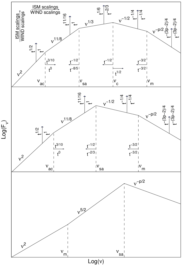
Figure 1: Fast cooling (FC) synchrotron spectra from a shock injected power law electron distribution. The shape of the spectrum is determined by the ordering of the self absorption frequency, $\nu_{sa}$, with respect to $\nu_{c}<\nu_{m}$. There are three possible shapes for the spectrum, corresponding to $\nu_{sa}<\nu_{c}$, $\nu_{c}<\nu_{sa}<\nu_{m}$ and $\nu_{sa}>\nu_{m}$, from top to bottom. Scalings for an afterglow, both in an ISM and wind environments, are given only in the first two frames, since for typical parameters $\nu_{sa}<\nu_{m}$ during the FC phase of the afterglow.

References

• Chevalier & Li (1999) Chevalier, R.A., & Li, Z.Y., 1999, preprint (astro-ph9908272)
• Crider et. al. (1998) Crider, A., et. al. , 1998, ApJ, 479, L39
• Fenimore et. al. (1996) Fenimore, E., et. al. , 1996, ApJ, 473, 998
• Ghisellini & Celotti (1999) Ghisellini, G., & Celotti, A., 1999, ApJ, 511, L93
• Granot, Piran & Sari (1999a) Granot, J., Piran, T. & Sari, R. 1999a, ApJ, 513, 679
• Granot, Piran & Sari (1999b) Granot, J., Piran, T. & Sari, R. 1999b, ApJ, 527, 236
• Katz (1994) Katz, J., 1994, ApJ, 432, L107
• Katz & Piran (1997) Katz, J. & Piran, T. 1997, ApJ, 490, 772
• Mészáros & Rees (1997) Mészáros, P. & Rees, M. 1997, ApJ, 476, 232
• Preece et. al. (1998) Preece, R.D., et. al., 1998, ApJ, 506, L23
• Sari, Narayan & Piran (1996) Sari, R., Narayan, R. & Piran, T. 1996, ApJ, 473, 204
• Sari & Piran (1997) Sari, R. & Piran, T. 1997, ApJ, 485, 270
• Sari & Piran (1999) Sari, R. & Piran, T. 1999, ApJ, 520, 641
• Sari, Piran & Narayan (1998) Sari, R., Piran, T. & Narayan, R. 1998, ApJ, 497, L17
• Strohmayer et. al. (1998) Strohmayer, T.E., et. al., 1998, ApJ, 500, 873
• Taylor et. al. (1998) Taylor, G.B., et al. 1998, ApJ, 502, L115
• Waxman (1997) Waxman, E., 1997, ApJ, 485, L5
• Wijers & Galama (1999) Wijers, R.A.M.J., & Galama, T.J. 1999, ApJ, 523, 177
Refer to caption