Generation of the Primordial Magnetic Fields during Cosmological Reionization

Abstract

We investigate the generation of magnetic field by the Biermann battery in cosmological ionization fronts, using new simulations of the reionization of the universe by stars in protogalaxies. Two mechanisms are primarily responsible for magnetogenesis: i) the breakout of I-fronts from protogalaxies, and ii) the propagation of I-fronts through the high density neutral filaments which are part of the cosmic web. The first mechanism is dominant prior to overlapping of ionized regions ($z\approx 7$), whereas the second continues to operate even after that epoch. However, after overlap the field strength increase is largely due to the gas compression occurring as cosmic structures form. As a consequence, the magnetic field at $z\approx 5$ closely traces the gas density, and it is highly ordered on megaparsec scales. The mean mass-weighted field strength is $B_{0}\approx 10^{-19}\mbox{\,G}$ in the simulation box. There is a relatively well-defined, nearly linear correlation between $B_{0}$ and the baryonic mass of virialized objects, with $B_{0}\approx 10^{-18}\mbox{\,G}$ in the most massive objects ($M\approx 10^{9}M_{\odot}$) in our simulations. This is a lower limit, as lack of numerical resolution prevents us from following small scale dynamical processes which could amplify the field in protogalaxies. Although the field strengths we compute are probably adequate as seed fields for a galactic dynamo, the field is too small to have had significant effects on galaxy formation, on thermal conduction, or on cosmic ray transport in the intergalactic medium. It could, however, be observed in the intergalactic medium through innovative methods based on analysis of $\gamma$-ray burst photon arrival times.

1 Introduction

The origin of magnetic fields in the universe is one of the most important unsolved problems in cosmology, and has possible ramifications for theories of galaxy formation and evolution (Wasserman 1978, Kim et al. 1996, Kulsrud et al. 1997) and for theories of the formation of the first stars (Yamada & Nishi 1998, Omukai & Nishi 1998, Abel et al. 1998, Nakamura & Umemura 1999, Bromm, Coppi, & Larson 1999); see also Rees (1987).

It is widely accepted that astrophysical magnetic fields reached their present state in a two stage process; first, the generation of a seed field, and then hydromagnetic processes which amplified the field or smoothed it. What are the possible sources for the origin of such seed field? The question has been posed repeatedly since the original work by Biermann (1950). Generally speaking, at least three different possible scenarios have been put forward. The first one assumes that a magnetic field is present ab initio: this does not violate homogeneity but makes the cosmological expansion anisotropic, and affects primordial nucleosynthesis via an increase of electron density. The field could have been generated either during QCD/electroweak first order cosmic phase transitions (Quashnock, Loeb & Spergel 1989, Vachaspati 1991) or during inflation (Turner & Widrow 1988, Ratra 1992). The upper limits on the present field strength obtained from CMB anisotropy measurements (Barrow, Ferreira & Silk 1997 give $B_{0}\leq 7\times 10^{-9}(\Omega h^{2})^{1/2}\mbox{\,G}$) appear to be more stringent than those derived from the Big Bang nucleosynthesis. The latter have been recently revised by Grasso & Rubinstein (1995), who found $B_{0}\leq 3\times 10^{-7}\mbox{\,G}$. The upper limit from CMB measurements comes very close to the minimum value ($\approx 10^{-9}\mbox{\,G}$) required for magnetic stresses to have been dynamically important (for example in the creation of voids, de Araujo & Opher 1997) in the post-recombination epoch. Compression alone, without a dynamo, would have brought such fields to the $\mu$G strengths characteristic of magnetic fields in galaxies. It is not clear that magnetic fields generated in the early universe possessed the degree of spatial coherence seen in galactic magnetic fields (Zweibel & Heiles 1997) but they could have been substantially reconfigured by turbulence and differential rotation in galaxies.

The second type of field generation mechanism would have operated prior to the recombination epoch, and was first proposed by Harrison (1970). This process invokes a Biermann battery (originally proposed for stars), i.e. nonparallel pressure and density gradients, powered by a non-zero vorticity in the primordial fluctuation field. Electrons and ions would have tended to spin at different rates due to the drag on electrons by the CMB. An ambipolar electric field would have arisen to couple the electrons and ions, and a magnetic field would thus have been created by induction. Zeldovich, Ruzmaikin, & Sokoloff (1983) later discussed a variant of this mechanism. Even if the vorticity is equivalent to galactic rotation by $z=10$, the magnitude of the resulting magnetic field is only of order $10^{-21}\mbox{\,G}$. However, vorticity modes are now thought to decay rapidly as irrotational modes grow and structure forms; thus this process now appears very unlikely.

In the third class of schemes, magnetic fields can arise during the epoch of protogalaxy formation, through any mechanism which produces a non-potential electric field. It is expected that fields produced in this manner must be small, and only act as a seed for a hydromagnetic dynamo. Two mechanisms for producing seed fields have been considered. In the first, magnetogenesis proceeds primarily in shocks. Davies & Widrow (1999) showed with simple analytic models that magnetic fields as high as $10^{-17}\mbox{\,G}$ can be generated during the collapse of protogalaxies. Kulsrud et al. (1997) computed the effect of the Biermann battery in a simulation of large scale structure. They found that magnetic fields are generated primarily in shocks associated with the gravitational collapse of the structure, with a a characteristic field strength of $10^{-21}\mbox{\,G}$.

In the second mechanism, magnetogenesis takes place in ionization fronts. Subramanian, Narasimha, & Chitre (1994, SNC) pointed out that the Biermann battery would operate in cosmological ionization fronts propagating through density irregularities. They made simple estimates based on the properties of protogalactic fluctuations, and suggested that fields of a few times $10^{-20}\mbox{\,G}$, with a coherence length of several kpc, could be generated by this mechanism. Along similar lines, but exploiting SN explosions rather than ionization fronts, Miranda, Opher & Opher (1998) concluded that field seeds as high as $B\approx 4.5\times 10^{-10}\mbox{\,G}$ can be created with coherence scales of order of $100$ kpc. However, their mechanism requires efficient SN shell fragmentation, which is not expected to occur in such low metallicity environments (Ferrara 1998). Furthermore, most of their magnetic flux is produced by objects with mass $\approx 10^{6}M_{\odot}$ forming at redshift $z\approx 300$, which is clearly at odds with all currently viable cosmological models.

We should also mention that battery mechanisms could have operated on much smaller scales, such as in accretion disks around massive compact objects, and seeded young galaxies and the IGM through outflows and jets (Daly & Loeb 1990).

Observations provide little guidance in choosing among these theoretical models. Attempts to determine intergalactic magnetic fields have yielded uncertain results, or at best upper limits. A very clean determination of primordial $B$-fields could be accomplished through measurement of Faraday rotation in the polarization of the CMB (Kosowsky & Loeb 1996). This will become possible with forthcoming experiments.

An experimental upper limit $B_{0}\lower 2.15277pt\hbox{$\;\buildrel<\over{\sim}\;$}10^{-9}(\Omega_{IGM}/0.01)\mbox{\,G}$ (see review by Vallée 1997 and references therein) is found on the intergalactic $B$-field averaged over a length scale comparable to the horizon. This upper bound would increase by a factor of 3 if the field were coherent on $10\mbox{\,Mpc}$ scales (Kronberg 1994).

Finally, there is some evidence for $\mu$G magnetic fields in young galaxies, as traced by high redshift (up to $z\approx 3$) quasars (Kronberg, Perry & Zukowsky 1990) and damped Ly$\alpha$ systems (Wolfe, Lanzetta & Oren 1992). This value might reflect the saturated level dictated by equipartition with turbulent energy (Field 1995), but it requires a rather high initial seed field value in order for the dynamo to amplify the field up to that strength. At that epoch, a dynamo working in a galaxy like the Milky Way should be provided a seed $B\lower 2.15277pt\hbox{$\;\buildrel>\over{\sim}\;$}10^{-18}-10^{-17}\mbox{\,G}$ (Beck et al. 1996).

The purpose of this paper is to explore magnetogenesis in cosmological ionization fronts using new simulations of the reionization of the universe by stars in protogalaxies. Our results include, in a self consistent manner, the wealth of density structures present at the epoch of galaxy formation (at least down to a scale imposed by numerical resolution). We corroborate the results of SNC to order of magnitude, place their suggestion on a firmer ground, isolate the most important mechanisms, and calculate the structure of the magnetic field in greater detail.

In §2 we describe the simulations, §3 gives the results, and §4 is a summary of the calculations and their limitations, as well as a discussion of their astrophysical relevance.

2 Method

2.1 Simulations

We use cosmological hydrodynamic simulations performed with the “Softened Lagrangian Hydrodynamics” (SLH) code and reported in Gnedin (2000). These simulations include 3D radiative transfer (in an approximate implementation) and are therefore suitable for following magnetic field generation. In addition, the simulations include a phenomenological description of the star formation process, based on the Schmidt law and on a full time-dependent treatment of atomic and molecular physics in a plasma with primeval composition.

Table 1: Numerical Parameters

Run	$N$	Box size	Baryonic mass res.	Spatial res.
A	$128^{3}$	$4h^{-1}{\rm\,Mpc}$	$10^{5.7}\mbox{\,M}_{\sun}$	$1.0h^{-1}{\rm\,kpc}$
B	$64^{3}$	$2h^{-1}{\rm\,Mpc}$	$10^{5.7}\mbox{\,M}_{\sun}$	$1.5h^{-1}{\rm\,kpc}$
C	$128^{3}$	$2h^{-1}{\rm\,Mpc}$	$10^{4.8}\mbox{\,M}_{\sun}$	$0.5h^{-1}{\rm\,kpc}$

We adopt a currently fashionable variant of the CDM+$\Lambda$ cosmological model with $\Omega_{0}=0.3$, $\Omega_{\Lambda}=0.7$, $h=0.7$, and $\Omega_{b}=0.04$. We have run three simulations with varying resolution, to estimate the level of numerical convergence. The numerical parameters of all three runs are listed in Table 1. Runs A and B are stopped at $z=4$ because at lower redshift the simulation box cannot be considered as a representative region of the universe: in fact, the rms density perturbation on the scale of the box size exceeds 0.25. Run C was stopped at $z=6.5$ because it is used for estimating numerical convergence only.

We will use run A as our reference run, whereas runs B and C will serve as a measure of the theoretical uncertainty of our calculations.

The placement of the simulation box of run A is designed in such a way as to marginally resolve the characteristic filtering scale below which the baryonic perturbations are smoothed due to the finite gas pressure. Thus, run A includes essentially all (about 93%) of the small scale power that is present in the initial conditions (Gnedin 2000). Since the small scale perturbations can contribute significantly to the total production rate of the magnetic field, we thus ensure that we do not miss a substantial portion of the total production in the regions with moderate overdensities. However, inside the virialized objects small scale power can be generated gravitationally, and since this power is not resolved, we are almost certainly underestimating the true value of the magnetic field. We argue below, however, that the magnetic field on large scales is generated primarily by structure on large scales. Thus, our calculation should produce a good approximation to the large scale fields produced by magnetogenesis in ionization fronts. The next stage, amplification of these primordial fields by dynamo action inside virialized objects, is outside the scope of this study.

2.2 Magnetic Field Equation

The evolution equation for the magnetic field with the Biermann battery source term can be written as follows:

$${\partial\vec{B}\over\partial t}+(\vec{v}\cdot\nabla)\vec{B}=-\vec{B}\mbox{\,div}\vec{v}+(\vec{B}\cdot\nabla)\vec{v}+{ck_{B}\over n_{e}e}\nabla T\times\nabla n_{e}+{{m_{e}c}\over{e}}\nu_{e\gamma}\nabla\times\vec{v}$$ (1)

where $n_{e}$ is the electron number density, $T$ is gas temperature, and

$$\nu_{e\gamma}={{4\sigma_{T}cU_{\gamma}}\over{3m_{e}c^{2}}},$$

with $U_{\gamma}$ being the energy density of the CMB, and $\sigma_{T}$ the Thompson cross section.

The left hand side of equation (1) describes a simple advection of the magnetic field together with the fluid. The two first terms on the right hand side of the field (induction) equation can be rewritten in index notation in the following form:

$$-B^{i}v^{j}_{,j}+B^{j}v^{i}_{,j}=-{2\over 3}B^{i}v^{j}_{,j}+B^{j}(v^{i}_{,j}-{1\over 3}\delta^{i}_{j}v^{k}_{,k})={2\over 3}B^{i}{D\rho\over dt}+B^{j}\sigma^{i}_{j},$$

where $D\rho/dt$ is the Lagrangian derivative of the gas density, and $\sigma^{i}_{j}$ is the traceless part of the velocity tensor. These two terms describe two physically different processes of amplification of the magnetic field : compression and stretching respectively. We discuss the importance of those two terms below. The third term in equation (1) is the Biermann battery, and the last term is due to Compton drag of CMB photons on the free electrons. We ignore the Hall effect and consider ions and neutrals moving with the same fluid velocity $\vec{v}$.

From general physical considerations, we expect that the battery term always dominates in ionization fronts, and is small everywhere else. It is useful to estimate the magnetic field produced by the battery term as an ionization front sweeps through the gas at speed $v_{f}$. Integrating equation (1) in time, keeping only the battery term and assuming that $\nabla n_{e}$ is in the direction of propagation of the front while $\nabla T$ is perpendicular to $\nabla n_{e}$ and is produced by some large scale inhomogeneity, we find

$$B\sim{{ck_{B}T}\over{ev_{f}l_{g}}},$$

where $l_{g}$ is gradient length scale for $T$. In order to get some physical feeling for this field strength, we introduce the ionization time $t_{i}\equiv l_{g}/v_{f}$, the ion gyrofrequency $\omega_{ci}\equiv eB/m_{i}c$, and the ion thermal velocity $v_{th}\equiv(k_{B}T/m_{i})^{1/2}$. In terms of these quantities,

$$\omega_{ci}t_{i}\sim{{v_{th}^{2}}\over{v_{f}^{2}}}.$$

Or, in terms of the thermal ion gyroradius $r_{i}\equiv v_{th}/\omega_{ci}$,

$$r_{i}/l_{g}\sim{{v_{f}}\over v_{th}}.$$

In contrast to the usual astrophysical situation, in which $\omega_{ci}^{-1}$ and $r_{i}$ are much smaller than any global time scales or length scales, the battery produces a field so weak that the magnetization scales and global scales are comparable. But note that small scale structure (small $l_{g}$) produces stronger fields.

The ratio of the photon drag term to the induction term, assuming that the vorticity is appreciable, is

$$\sim{{\nu_{e\gamma}}\over{\omega_{ce}}},$$ (2)

where $\omega_{ce}\sim 10^{7}B\mbox{\,s}^{-1}$ is the electron gyrofrequency. Since $\nu_{e\gamma}=5\times 10^{-20}(1+z)^{4}\mbox{\,s}^{-1}$, the induction dominates photon drag for

$$B>5\times 10^{-27}(1+z)^{4}\mbox{\,G}.$$ (3)

Using the outputs from the simulations, we solved equation (1) numerically using clouds-in-cells (Efstathiou et al. 1985) to advect the right hand side of equation (1) over the SLH quasi-Lagrangian mesh, and implementing the Lax averaging for the stretching term to ensure the stability of the scheme. We chose the time-step so as to ensure numerical convergence with respect to time discretization.

We ignore the back reaction of the magnetic field because the magnetic pressure for the field strength we obtain ($B\sim 10^{-19}\mbox{\,G}$, $B^{2}/8\pi\sim 10^{-40}\mbox{\,erg}/\mbox{\,cm}^{3}$) is far smaller than the gas pressure even in the low density IGM ($P\sim 10^{-16}\mbox{\,erg}/\mbox{\,cm}^{3}$ at $z\sim 7$).

3 Results

3.1 General Outlook

Figure 1: Evolution of the mass (bold lines) and volume (thin lines) weighted mean magnetic field strength (top panel) and the comoving mean free path to ionizing radiation (bottom panel) for runs A (solid lines), B (dotted lines), and C (dashed lines).

We can now look at general features of the magnetic field generated during the reionization. Figure 1 shows the evolution of the mass and volume weighted mean magnetic field strength as well as the mean free path to ionizing radiation for all three simulations discussed in this paper. The difference between the curves illustrates the level of numerical convergence achieved in the simulations, and can be considered the theoretical error of our simulations. In particular, the differences at high redshift are due to the fact that our reference run A simulation still misses some 7% of the small scale power, which translates into a $\approx 15$% shift in redshift. However, the saturation levels of all three runs are about the same. Since run C has a twice smaller cell size (and, therefore, approximately four times less numerical diffusion), the agreement in the saturated level of the produced magnetic field demonstrates that numerical diffusion does not lead to a substantial underestimate of the magnetic field strength produced in our simulations. This test is not however completely conclusive because of the excess small scale power present in run C, and therefore we cannot exclude the possibility that numerical diffusion affects our results on a several tens of percent level. However, since we focus in this paper on the general semi-qualitative description of the generation of the primordial magnetic field, we can tolerate a factor of two uncertainty in our calculations.

We point out here that the mean field strength generated in our simulations exceeds the value found by Kulsrud et al. (1997) by about two orders of magnitude. We will elaborate on this difference in the next subsection.

The evolution of the mean field clearly exhibits two distinct regimes: before the overlap of the ${\rm H\,\sc ii}$ regions at $z=7$ (characterized by a sharp increase in the mean free path of ionizing photons) the mean field grows with time, but after the overlap its growth slows down appreciably.

Figure 2: Evolution of the mass (bold lines) and volume (thin lines) weighted mean magnetic field strength in the full calculation (solid lines), with the Compton drag term omitted (long-dashed line), with the stretching and the Compton drag terms omitted (short-dashed line), and with the compression and the Compton drag terms omitted (dotted line).

We attempt to understand this behavior by considering which terms in equation (1) are dominant at a given time. Figure 2 shows four solutions to equation (1) for the large simulation: the solid lines mark the full solutions (either mass- or volume-weighted), the same one as shown in the previous Figure; the long-dashed line shows a solution with the Compton drag term omitted; the dashed line shows a solution with both the Compton drag term and the stretching term omitted; and the dotted line shows a solution with both the Compton drag term and the compression term omitted. We can immediately conclude that stretching by itself makes an insignificant contribution, whereas compression is the dominant term after the overlap of the ${\rm H\,\sc ii}$ regions, and the Biermann battery is responsible for the initial growth of the field during the pre-reionization stage. The Compton drag term is only important for $z>16$, when the magnetic field is less than about $5\times 10^{-23}\mbox{\,G}$. Using the estimate (3) we find that at this moment the induction term is about 10% of the Compton drag, and the comparison between the dotted and solid lines in Fig. 2 shows that the Biermann battery at that time is on average about 10 times more important than the induction term, in agreement with our estimate (3).

Figure 3: The joint mass-weighted distribution of the gas density and the magnetic field strength at $z=4$.

Since compression is the dominant term at lower redshifts, we expect that the magnetic field has to be closely related to the gas density. The battery term has a similar effect, as ionization fronts tend to move slowly in regions of high gas density. Figure 3 illustrates this point. In this Figure we show the joint mass-weighted distribution of the gas density and the magnetic field strength for all fluid elements in the large simulation. As one can see, there is a strong correlation between the gas density and the magnetic field, albeit with a considerable (two orders of magnitude in magnetic field strength) scatter. The most probable value for the magnetic field strength (the peak of the distribution) rises with density slightly more steeply than the first power. We will give an explanation for this feature in the next subsection, where we discuss the main mechanism for generating the primordial magnetic field.

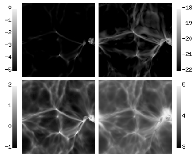
Figure 4: A thin slice through the simulation volume at $z=4$, showing in four panels the logarithm of the neutral hydrogen (upper-left) and the gas density (lower-left) (in units of the average density of the universe), the gas temperature (lower-right), and the magnetic field strength (upper-right).

In Figure 4 we show a thin slice through the simulation box taken at a random place. In four panels we show the gas density, temperature, neutral fraction, and the magnetic field strength (all stretched logarithmically). Again, visual inspection demonstrates that the magnetic field is strongly correlated with the gas density. It is also correlated with the gas neutral fraction and the temperature, as these quantities also correlate with the gas density in the moderate density regime (cosmic overdensity $\delta\lesssim 10$).

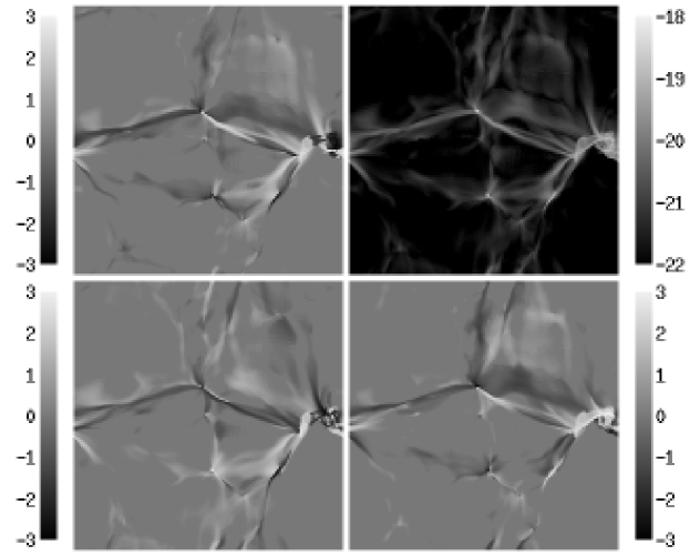
Figure 5: A thin slice through the simulation volume at $z=4$, showing the magnetic field strength in the upper-right panel (just as in Fig. 4) and three components of the magnetic field in the other three panel.

Finally, in Figure 5 we show the magnetic field strength again (just as in Fig. 4) together with the three cartesian components of the magnetic field. Since the components can be both positive and negative, we use the following stretch to map the value of the component in the range from $-10^{-19}\mbox{\,G}$ to $+10^{-19}\mbox{\,G}$ to a quantity in the range from $-3$ to $+3$:

$${\rm stretch}=\mbox{\,sign}(B_{i})\mbox{\,log}(1+10^{22}\mbox{\,G}^{-1}|B_{i}|).$$

As one can see, the magnetic field is highly ordered on scales of the order of $1\mbox{\,Mpc}$, and magnetic structure is highly correlated with density structure. As pointed out above, this is the result of the compression occurring as cosmic structures form. As we have already discussed, this is not an artifact of finite numerical resolution, since our simulation resolves all the relevant scales in the moderate density regime. Only inside the virialized clumps do we encounter scales which we are unable to resolve, and there our calculation of the magnetic field strength becomes a lower limit, on top of which small scale dynamo processes will generate additional field on galactic and subgalactic scales. Since these latter processes cannot be simulated reliably with the current resolution of our simulations, we cannot consider them in this paper. On the other hand, the extragalactic magnetic fields are calculated reliably in our simulations for a given cosmological model.

3.2 Main Mechanisms for Generating the Magnetic Field

Since the Biermann battery is most efficient when the gradient of the electron density is perpendicular to the temperature gradient, we can identify two main mechanisms where the battery is most efficient. But before we can do so, let us briefly describe the main stages of reionization (Gnedin 2000). We also point out that the reionization process is affected by several feedback mechanisms which are discussed in Ciardi et al. (2000).

The reionization starts with ionization fronts propagating from proto-galaxies located in high density regions into the voids, leaving the high density outskirts of the protogalaxies still neutral, because at high density the recombination time is very short, and there are not enough photons to ionize the high density regions. As an ionization front expands into previously neutral material, it leaves behind high density regions whose ionization requires more photons than currently available. This stage of the reionization process can be called “pre-overlap”, and it extends over a considerable range of redshifts $\Delta z\sim 5$ around $z\sim 10$. During this time the high density regions close to the source slowly become ionized, whereas more distant high density regions remain neutral.

By $z\approx 7$ (for the cosmological model under consideration) the ${\rm H\,\sc ii}$ regions start to overlap. As a result, an average place in the universe can see an increasing number of sources, and the ionizing intensity starts to rise rapidly. The process of reionization enters its second stage, the “overlap”, which is quite rapid ($\Delta z\sim 1$). As the ionizing intensity is rapidly increasing, the last remains of the neutral low density IGM are quickly eliminated, the mean free path increases by some two orders of magnitude over a Hubble time or so (see Fig. 1), and voids become highly ionized (neutral fraction of the order of $10^{-5}$). The high density regions at this moment are still neutral, as the number of ionizing photons available is not sufficient to ionize them.

After the overlap is complete, the universe is left with both highly ionized low density regions and some of the high density regions (which happened to lie close to the source, where the local value of the ionizing intensity is higher than the background). High density regions far from any source remain neutral. This stage can be called “post-overlap”. As time goes on, and more and more ionizing photons are emitted, the high density regions are gradually eaten away.

Figure 6: A cartoon, illustrating the mechanism for generating the primordial magnetic field during the break through of the I-front from the proto-galaxy before the overlap of the ${\rm H\,\sc ii}$ regions. Enclosed contours show the regions of progressively higher density.

Figure 6 shows now a cartoon version of the first out of two most important mechanisms for generating the primordial magnetic field. The mechanism takes place when the first I-front breaks through the protogalaxy. This happens first in a narrow range of angles, where the gas density happens to be the lowest. As the I-front propagates into the low density IGM, the gradient of the electron density (the surface of the I-front) becomes approximately orthogonal to the temperature gradient, and the battery becomes maximally efficient.

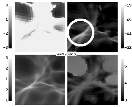
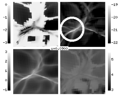
Fig. 7a Fig. 7b

Figure 7: A thin slice through the simulation volume similar to Fig. 4 but showing $1/5$th of the box ($0.8h^{-1}\mbox{\,Mpc}$ on a side), aimed at illustrating the generation of the magnetic field during the break-through of the I-front. Two redshifts are shown: $z=11.5$ (a) and $z=10.1$ (b). The region around the I-front is emphasized by the white circle.

Figure 7 illustrates this mechanism with an example from the simulation. Each of the frames is similar to Fig. 4, except that it is only one fifth the box size ($0.8h^{-1}\mbox{\,Mpc}$) on a side. Two panels show a protogalaxy just before and after the I-front broke through the gaseous halo. The magnetic field has increased by almost an order of magnitude during the short time interval ($\Delta t=75\mbox{\,Myr}$) between the two snapshots.

The magnetic field produced by this mechanism has toroidal topology, wrapping around the ${\rm H\,\sc ii}$ region. This can be seen by inspection of the battery term: $\nabla n_{e}$ is directed across the ionization front, while $\nabla T$ follows the large scale stratification of the protogalaxy and is directed along the major axis of the cone shaped H II region. The magnetic field is oriented along the cross product of these gradients, i.e. the field encircles the H II region. The reversal of the out-of-plane component of the field across the H II region is indeed observed in the simulation.

Figure 8: A cartoon, illustrating the second mechanism for generating the primordial magnetic field during reionization: the I-front crossing a neutral high density filament after the epoch of overlap. Enclosed contours show the regions of progressively higher density.

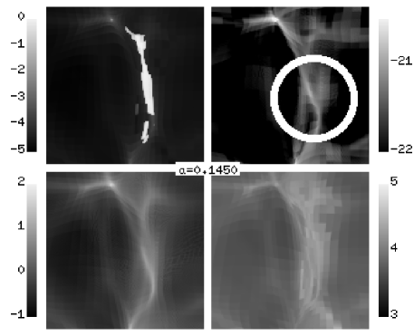
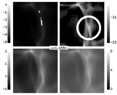
Fig. 9a Fig. 9b

Figure 9: A thin slice through the simulation volume similar to Fig. 4 but showing $1/25$th of the box ($0.8h^{-1}\mbox{\,Mpc}$ on a side), illustrating the generation of the magnetic field during the propagation of the I-front across the high density filament. Tho redshifts are shown: $z=5.9$ (a) and $z=5.5$ (b). The region around the I-front is emphasized by the white circle.

The second mechanism is important when the I-front propagates across the high density neutral filament. This is shown in Figure 8 as a cartoon version and further illustrated in Figure 9 with two snapshots from the simulation. Both, the cartoon and the snapshots, demonstrate how this mechanism operates in the post-overlap stage, when the low density IGM is already ionized. However, it is clear from the cartoon that the ionization state of the surrounding low density IGM is irrelevant, and that this mechanism works in the pre-overlap stage as well, when the filament is embedded in the neutral rather than ionized gas. In general, however, I-fronts propagate much more slowly across the high density filaments than in the low density IGM, so it is likely that the IGM around the filament is already ionized when the I-front propagates across it.

It is important to keep in mind that the filaments are neutral not because they are self-shielded, but because they are dense enough for the recombination time to be shorter than the photoionization time, i.e. even if filaments are neutral, they are nevertheless photoheated. Since in the IGM with moderate overdensities ($\delta\lesssim 10$) there exists a tight relation between the gas density and the gas temperature (the so called “effective equation of state”, Hui & Gnedin 1998), even a filament with quite moderate overdensity has a temperature gradient pointed outward, the most efficient orientation for Biermann battery.

The first mechanism operates during the formation of a virialized objects, i.e. in higher density environments than the second mechanism. This fact explains why the field increases with density faster than $\rho^{2/3}$, which would be the predicted law if the simple compression were the dominant term in equation (1). Since high density regions collapse first, the field per unit mass inside the protogalaxies is larger than the field per unit mass in the lower density filaments and the IGM.

The existence of these two mechanisms is also the source of our disagreement with Kulsrud et al. (1997), who found fields which are two orders of magnitude less than the value we find. Since Kulsrud et al. (1997) did not include radiative transfer in their simulations, they were not able to follow the I-fronts, and therefore completely missed these two important mechanisms for field generation. Their field was therefore generated by chance misalignments between the electron density and temperature gradients. These misalignments are also present in our simulations, but they can be a dominant source of the magnetic field only in the low density IGM, where none of the mechanisms described above operates. Thus, in the low density IGM we should be finding values for the magnetic field strength similar to the ones found by Kulsrud et al. (1997), i.e of the order of $10^{-21}\mbox{\,G}$, which is indeed the case, as can be seen from Fig. 3.

3.3 Primordial Field in the Protogalaxies

As we have mentioned above, our simulations do not have enough resolution to model the interstellar medium, and therefore cannot describe the field generation in the galactic ISM. Thus, the values of the magnetic field strength that we find inside the protogalaxies should only be considered as the truly primordial field, generated during the period of reionization. The true field inside the protogalaxies at, say, $z=4$, could be significantly higher than the values we obtain (of the order of $10^{-18}\mbox{\,G}$), although it would be coherent only on small scales. Here, we have in mind small scale fields generated directly by the battery mechanism, as ionization fronts propagate through the clumpy molecular clouds in which stars are born. However, these small scale fields do not contribute as much to the magnetization of protogalaxies as large scale fields do, as we show by the following rough argument.

Suppose that the battery acts on small clouds or filaments of characteristic size $D_{o}$ and density $n_{c}$, and produces a field $B(D_{o})$. If most of the mass in the star-forming complex is in these small clumps, then when the clumps eventually disperse their mean size will be $D\sim D_{o}(n_{c}/\langle n\rangle)^{1/3}$, where $\langle n\rangle$ is the mean interstellar density. Because of conservation of magnetic flux, the magnetic field in the dispersed clumps is $B(D)\sim B(D_{o})(\langle n\rangle/n_{c})^{2/3}$. Space is then divided into independent magnetic domains of size $D$, and the fields within the domains are randomly oriented with respect to one another. Over a region of size $l>D$, a random walk argument shows that $B(l)\sim B(D)(D/l)^{3/2}$ (Hogan 1983). In terms of the original battery field, $B(l)\sim B(D_{o})(\langle n\rangle/n_{c})^{1/6}(D_{o}/l)^{3/2}$.

We now compare $B(l)$ computed as the sum of fields in small domains with the coherent field $B_{c}(l)$ which is generated by propagation of a single I-front. From the scaling of the battery with system size and I-front velocity $v_{f}$ we expect $B_{c}(l)\sim B(D_{o})(D_{o}/l)[v_{f}(D_{o})/v_{f}(l)]$. The ratio $B_{c}(l)/B(l)$ is then $B_{c}(l)/B(l)\sim(l/D_{o})^{1/2}(n_{c}/\langle n\rangle)^{1/6}[v_{f}(D_{o})/v_{f}(l)]$. This expression shows that unless the ionization fronts in the clumps propagate much more slowly than the fronts on large scales, the coherent field dominates the superimposed incoherent fields. Although the clumps can be very dense, which slows down the fronts, they are also much closer to the source of ionization, which speeds them up. Therefore, the ionization front battery on large scales is more important for the generation of a galactic field than the battery on the scale of molecular clumps in star forming regions. However, if the locally generated battery field is amplified sufficiently rapidly to equipartition with the turbulence, it could play a role in subsequent generations of star formation in the protogalaxy.

Since we follow the intergalactic field with sufficient precision, we can separate the whole problem of the generation of the magnetic field into two distinct phases: the formation of the primordial field during reionization, which we can reproduce with our simulations, and the dynamo action inside the protogalaxies, which we cannot resolve. The latter process, though, is restricted to the protogalaxies only, and therefore could be, at least to a first approximation, considered independently from the rest of the universe.

Figure 10: Evolution of the stellar mass (upper-left), the gas mass (upper-right), the rms magnetic field strength (lower-left), and the absolute value of the mean $z$-component of the magnetic field of the most massive virialized object within the $4h^{-1}\mbox{\,Mpc}$ simulation box (solid lines), the 10th most massive object (long-dashed lines), the 50th most massive object (dot-dashed lines), and the 250th most massive object (dotted lines).

Figure 10 shows the time evolution of the stellar mass, the gas mass, the rms magnetic field strength and the absolute value of the mean $z$-component of the magnetic field ($x$- and $y$- components look very similar) for four representative objects from our simulation. We notice that the rms field traces the evolution of the mean cosmic field from Fig. 1, and saturates at the values of about $(1-2)\times 10^{-18}\mbox{\,G}$ in the most massive objects. The absolute value of the $z$-component is about 10 times smaller, implying that only 10% of the total field is in an ordered state over the scale of an object.

Figure 11: The final rms magnetic field strength versus baryonic mass for all virialized objects from our simulation.

Finally, in Figure 11 we show the final (i.e. saturated) value of the rms magnetic field strength versus mass for all virialized objects from our simulation. The most massive objects with baryonic mass in the range $10^{9}-10^{10}\mbox{\,M}_{\odot}$ all have rms magnetic field strength about $10^{-18}\mbox{\,G}$ with a factor of a few scatter. One can also notice a correlation between the baryonic mass and the rms magnetic field strength, albeit the scatter is quite large. This correlation occurs for the same reason as the steep $B$ vs. $\rho$ dependence: the I-fronts are more efficient in producing magnetic fields while they are breaking through the neutral halos of the protogalaxies than when they are propagating across filaments.

4 Conclusions

We have studied the generation of magnetic field during the reionization of the universe outlining the main mechanisms, arising in ionization fronts, responsible for magnetogenesis. Our results allow us to conclude that the cosmic seed magnetic field closely traces the gas density, and that it is highly ordered on megaparsec scales, with a mean strength $B_{0}\approx 10^{-19}\mbox{\,G}$. We find that in protogalaxies the field is an order of magnitude or more larger than the mean field; this is an upper limit because unresolved small scale structure in the protogalaxies could generate stronger fields, and amplify them rapidly.

The magnetogenesis mechanism proposed here owes its robustness to both the relatively simple physics involved (i.e. ionization fronts) and the strong experimental evidence that reionization of the universe has indeed occurred. Although we have assumed here that reionization is driven by stellar sources, which appears to be consistent with available experimental data on the metallicity of the IGM (Gnedin & Ostriker 1997; Ferrara, Pettini & Shchekinov 2000), quasars – if present prior to reionization – are likely to produce a similar effect as they ionize the surrounding intergalactic medium.

This field strength is about 10 orders of magnitude too small to have a dynamical effect on galaxy formation. One way to see this is to recognize that the Alfven speed in a medium with $n=10^{-4}\mbox{\,cm}^{-3}$, $B=10^{-19}\mbox{\,G}$ is $2\times 10^{-6}\mbox{\,cm}/\mbox{\,s}$. This field is also too small to have much effect on microscopic transport processes such as thermal conductivity. The relevant parameter here is $\omega_{c}\tau_{c}$, where $\omega_{c}$ and $\tau_{c}$ are the gyrofrequency and Coulomb collision time, respectively, and their product must exceed unity for thermal conduction to be suppressed. In a plasma with $n=10^{-4}\mbox{\,cm}^{-3}$, $T=10^{5}\mbox{\,K}$, $B=10^{-19}\mbox{\,G}$, this parameter is about $3\times 10^{-3}$ for electrons. Similarly, the gyroradius of a high energy cosmic ray propagating through this field is extremely large: a $10^{19}\mbox{\,eV}$ proton in a $10^{-19}\mbox{\,G}$ magnetic field has a gyroradius of $10^{11}\mbox{\,Mpc}$, so high energy intergalactic cosmic rays would be essentially unmagnetized.

However, such a field, even reduced by $(1+z)^{2}$ from its value at formation, might be detectable through its effects on the arrival times of $\gamma$-rays from extragalactic sources (Plaga 1995, Lee, Olinto, & Sigl 1995, Waxman & Coppi 1996). The effect of the field on the polarization of the CMB would be much less than that modeled by Kosowsky & Loeb (1996), who required fields 9-10 orders of magnitude larger to find a detectable magnetic signature.

This field could explain the strength currently observed in the Milky Way and in external galaxies, provided it is further amplified by a some other process, as for example a dynamo which has exponentiated 30 times. The protogalactic seed fields are just barely large enough to have been amplified by a dynamo to $\mu$G strengths by $z\sim 1$, as suggested by the observations of damped Ly$\alpha$ systems.

References

- (1)
- (2) Abel, T., Anninos, P., Norman, M. L., & Zhang, Y. 1998, ApJ, 508, 518
- (3)
- (4) Balbus, S. A. 1993, ApJ, 413, 137
- (5)
- (6) Barrow, J. D., Ferreira, P. G., & Silk, J. 1997, Phys. Rev. Lett., 78, 3610
- (7)
- (8) Beck, R., Brandenburg, A., Moss, D., Shukurov, A., & Sokoloff, D. 1996, ARA&A, 34, 155
- (9)
- (10) Biermann, L. 1950, Z. Naturf. A., 5, 65
- (11)
- (12) Bromm, V., Coppi, P. S., & Larson, R. B. 1999, ApJ, 527, L5
- (13)
- (14) Ciardi, B., Ferrara, A., Governato, F., & Jenkins, A. 2000, MNRAS, in press (astro-ph/9907189)
- (15)
- (16) Daly, R.A., & Loeb, A. 1990, ApJ, 364, 451
- (17) Davies, G., & Widrow, L. M. 1999, ApJ, in press (astro-ph/9912260)
- (18)
- (19) de Araujo, J. C. N., & Opher, R. 1997, ApJ, 490, 488
- (20)
- (21) Efstathiou, G., Davis, M., Frenk, C. S., & White, S. D. M. 1985, ApJS, 57, 241
- (22)
- (23) Ferrara, A. 1998, ApJ, 499, L17
- (24)
- (25) Ferrara, A., & Shchekinov, Yu. 1996, ApJ, 465, L91
- (26)
- (27) Ferrara, A., Pettini, M., & Shchekinov, Yu. 2000, MNRAS, submitted
- (28)
- (29) Field, G. B. 1995, The Physics of the Interstellar Medium and the Intergalactic Medium, ASP Conf. Ser. 80, eds. A. Ferrara et al. , (San Francisco: PASP)
- (30)
- (31) Gnedin, N. Y., & Ostriker, J. P. 1997, ApJ, 486, 581
- (32)
- (33) Gnedin, N. Y. 2000, ApJ, in press (astro-ph/9909383)
- (34)
- (35) Grasso, D., & Rubinstein, H. R. 1995, Astroparticle Physics, 3, 95
- (36)
- (37) Harrison, E. R. 1970, MNRAS, 147, 279
- (38)
- (39) Hogan, C. L. 1983, Phys. Rev. Lett., 51, 1488
- (40)
- (41) Hui, L., & Gnedin, N. Y. 1998, MNRAS, 292, 27
- (42)
- (43) Kim, E., Olinto, A., & Rosner, R. 1996, ApJ, 468, 28
- (44)
- (45) Kosowsky, A., & Loeb, A. 1996, ApJ, 469, 1
- (46)
- (47) Kronberg, P. P. 1994, Rep. Prog. Phys., 57, 325
- (48)
- (49) Kronberg, P. P., Perry, J. J., & Zukowsky, E. L. H. 1990, ApJ, 355, L31
- (50)
- (51) Kulsrud, R. M., & Andersson, S. W. 1992, ApJ, 396, 606
- (52)
- (53) Kulsrud, R. M., Cen, R., Ostriker, J. P., & Ryu, D. 1997, ApJ, 480, 481
- (54)
- (55) Lee, S., Olinto, A. V., & Sigl, G. 1995, ApJ, 455, L21
- (56)
- (57) MacLow, M. M., & Ferrara, A. 1999, ApJ, 513, 142
- (58)
- (59) Miranda, O. D., Opher, M., & Opher, R. 1998, MNRAS, 301, 547
- (60)
- (61) Nakamura, F., & Umemura, M. 1999, ApJ, 515, 239
- (62)
- (63) Omukai, K., & Nishi, R. 1998, ApJ, 508, 141
- (64)
- (65) Quashnock, J. M., Loeb, A., & Spergel, D. N., 1989, ApJ, 344, L49
- (66)
- (67) Plaga, R. 1995, Nature, 374, 430
- (68)
- (69) Ratra, B. 1992, ApJ, 391, L1
- (70)
- (71) Rees, M. J. 1987, QJRAS, 28, 197
- (72)
- (73) Subramanian, K., & Barrow, J. D. 1998, Phys. Rev. Lett., 81, 3575
- (74)
- (75) Subramanian, K. & Narasimha, D., & Chitre, S. M. 1994, MNRAS, 271, L15 (SNC)
- (76)
- (77) Turner, M. S., & Widrow, L. M. 1988, Phys. Rev. D, 37, 2743
- (78)
- (79) Vachaspati, V. 1991, Phys. Lett. B, 265, 258
- (80)
- (81) Vallée, J. P. 1990, ApJ, 360, 1
- (82)
- (83) Vallée, J. P. 1997, Fund. Cosm. Phys., 19, 1
- (84)
- (85) Waxman, E., & Coppi, P. 1996, ApJ, 464, L75
- (86)
- (87) Wasserman, I. 1978, ApJ, 224, 337
- (88)
- (89) Wolfe, A. M., Lanzetta, K. M., & Oren, A. L. 1992, ApJ, 388, 17
- (90)
- (91) Yamada, M., & Nishi, R. 1998, ApJ, 505, 148
- (92)
- (93) Zeldovich, Ya. B., Ruzmaikin, A. A., & Sokoloff, D. D. 1983, Magnetic Fields in Astrophysics, (New York: Gordon & Breach)
- (94)
- (95) Zweibel, E. G., & Heiles, C. 1997, Nature, 385, 131
- (96)