Photometric modal discrimination in Scuti and Doradus stars
Abstract
The potential of photometric methods for the identification of , the degree of spherical surface harmonic of a pulsating star, is investigated with special emphasis on Strömgren photometry applied to Scuti and Dor variables. Limitations of actual model atmospheres when fine precision is required for the calculations of partial derivatives and integrals, which depend on limb darkening coefficients, are discussed. Two methods are discussed to calculate the phase lags, the angle between maximum temperature and minimum radius, and , a parameter which describes departure from adiabaticity of the atmospheres of these pulsating stars. These quantities appear to be very dependent on the convection as parametrized by the mixing length theory. When one of the methods is applied to the Dor stars gives phase lags close to , which are out of phase from typical Scuti stars. Examples are given for some High Amplitude Delta Scuti Stars (HADS) where the method can be easily applied and gives results consistent to interpret them as radial (=0) pulsating stars. Other low amplitude Scuti stars could be oscillating in a non-radial (=1, 2) mode. Multi-band photometry is concluded to be a very powerful tool for mode identification of Scuti and Dor stars, specially with the more accurate photometry that will be achieved in the near future with the asteroseismological space missions now in progress.
Instituto de Astrofisica de Andalucia, C.S.I.C., Apdo. 3004, 18080, Granada, Spain
1. Introduction
In recent years the development of photometric multi-site campaigns organized by different teams: Delta Scuti Network (http://dsn.astro.univie.ac.at), STEPHI (http://dasgal.obspmfr/stephi/) and STACC (Frandsen et al. 1996) for studying multi-periodic Scuti stars has increased the number of detected frequencies up to a level at which we could think that direct fitting to a theoretical model could be relevant to test the modelization and finally to do real asteroseismology of these stars. See for instance Breger et al. (1999) for FG Vir and Pamyatnykh et al. (1998) for XX Pyx. However the number of theoretically excited and photometrically visible radial and non-radial periods in a Scuti is so large that it is impossible to match all theoretical frequencies to the observed ones. For this reason a method to identify modes is needed. One can think that the rotational splitting is the most simple method and to look for singlets (radial, ), triplets (dipole, ), etc., in the frequency spectrum. However the overlapping and non-linear interactions among them destroy the expected regular pattern as demonstrated in Breger et al (1999). In any case some residual regularity can be expected and used as an indication of the degree of the spherical harmonic of the observed modes, as explained there. Therefore identification of at least a few frequencies becomes necessary to attempt to make asteroseismological techniques available for Scuti stars.
Another approach, better explained in other reviews of this conference, consists of the use of the line profile variations to model the surface velocity field and then deduce the corresponding spherical harmonic. Technical details are given elsewhere, Mantegazza in these proceedings and Aerts these proceedings as well, but I would like to note here the difficulty to get sufficient spectroscopic measurements, since both high S/N ratio and time coverage to resolve frequencies are required, so that medium size telescopes are needed. In fact it is quite difficult to organize multi-site spectroscopic campaigns for many days, but easier when the same is done for small photometric telescopes. However the enormous advantage of the spectroscopy is that one can obtain information not only on the -values but also on the azimuthal order of the spherical harmonic -values, which are not detectable from purely photometric observations.
The main question we want to address here is whether multi-band photometry alone can be useful to discriminate -values or not.
Based on the linearization made by Dziembowski (1977) of the bolometric magnitude variations exhibited by a star undergoing non-radial oscillations, Balona & Stobie (1979a, 1979b) formulated an analytic expression which will be used throughout this review in the form given by Watson (1988). The equation, as we will see later on, contains evaluations of flux derivatives and of integrals over limb darkening coefficients. This requires a well-behaved model atmospheres not only describing mean values, from which we can deduce physical parameters, but also their variations as far as temperature and/or gravity varies.
I will start by introducing the linearized equation and the physical conditions required for applicability, then I will discus the limitations of the available model atmospheres, basically Kurucz models and modifications, concerning partial derivatives and limb darkening coefficients. As we will see, there are two unknown quantities in the formula, the phase lag and a parameter related with departures from adiabaticity, which deserves a detailed discussion given in section 3. The next section is devoted to the application to real data mainly through the use of Strömgren photometry. Finally in the last section, I will present the expected possibilities of the method in the context of future space missions.
2. The linearized equation
Thermal time scales for Scuti stars are at least an order of magnitude larger than the shortest observed period. Furthermore the relative radius variations, even for the High Amplitude Scuti Stars (HADS), are so small that second order terms can be neglected.
Under such conditions the linearized equation governing the photometric variation of a pulsating star, , can be expressed, following the formulation given in Watson (1988), as:
| (1) | |||||
where the variables have the following definitions:
-
•
the ’s stand for the different photometric bands. Here I will use and of the Strömgren photometric system.
-
•
is an arbitrary small quantity.
-
•
is the associated Legendre polynomial of order to the pulsation frequency , oriented with the angle , i. e. the inclination of the stellar pulsation axis to the observer.
-
•
is the Phase Lag, i.e. the angle between maximum temperature and minimum radius, hence in perfect adiabatic conditions.
-
•
The can be written as follows:
(2) (3) (4) (5) (6)
where are the weighted limb darkening integrals defined as:
| (7) |
where, using a quadratic limb darkening law,
| (8) |
Partial derivatives and limb darkening coefficients have to be tabulated from theoretical model atmospheres. is a measure of the variation of the pressure when a gravity variation occurs, evaluated at an optical layer where we observe the continuum flux. It is then
| (9) |
From model atmospheres and in the Scuti regime this value can be considered as a constant equal to approximately 1.4.
and are related by the equation:
| (10) |
where is given by:
| (11) |
and
| (12) |
is calibrated, see for instance Breger et al. (1993), using the following equation:
| (13) |
Standard photometric indices are then used to calibrate gravity, absolute magnitude and temperature and, by knowing the pulsation period, we can obtain the observational value for the pulsation constant .
is introduced as a free parameter to estimate deviations from adiabaticity, since for an adiabatic atmosphere:
| (14) |
then must be unity in that case and physical values for must be between and . The adiabatic exponent can show dramatic changes in the atmosphere of a pulsating star but in our case we assume a constant value of . So any change of this parameter will change the value of , which will remain as an unknown parameter in equation (1).
The general procedure described here to obtain -values from observed photometric indices is explained in the flow chart of Fig 1. It is based on the use of model atmospheres to calculate not only global physical quantities for a given star but also variations of the photometric indices with respect to temperature and gravity, together with the above defined integral of the limb darkening coefficients. However, and in order to know the corresponding -value, we need to have an estimation of the two unknown variables and . Before doing that in the next section we will discuss more in detail the precision of these quantities when model atmospheres from Kurucz (1993), i.e. ATLAS9 code, are used.
Starting by the observables , the calibrated photometric indices, , the pulsation period and the time variations of the photometric indices , , which include phases and amplitudes, we are able to obtain for the Scuti and related stars the following:
-
1.
Effective temperatures, gravity and metallicity from model atmospheres
-
2.
Limb darkening coefficients and partial derivatives, also from model atmospheres
-
3.
Pulsation constant from equation (13) and the previously calibrated quantities
There are three quantities which remain unknown from equation (1): the phase lag, , the adiabaticity parameter, , and the -value we are searching for. At this point two strategies exist:
-
•
to make an assumption with physical sense about and . Usually is selected in the range only from theoretical considerations whereas is selected in the range of from spectroscopic observations of Scuti stars. One can draw then the corresponding “regions of interest” for the different -values. A comparison of the phase differences vs. amplitude ratios with observations is the approach followed by different authors (Watson, 1988 and Garrido et al., 1990).
-
•
to estimate and either from theoretical calculations (Balona and Evers, 1999) or by photometric observations as explained in detail in Garrido et al. (1990).
In both cases the final estimation of the -value is made by selecting, through a least squares procedure, the minimum distance between predictions and observations as we will see in section 5.2.
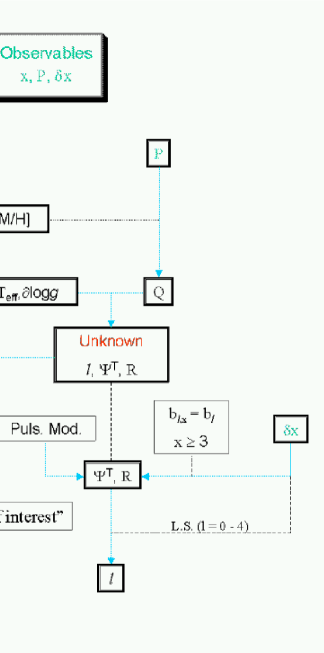
Following the flow chart in Fig 1 we will next discuss in detail a practical application by using Strömgren data and Kurucz models.
3. Kurucz model atmospheres
3.1. Physical calibration
The Strömgren system is a photometric system composed of 4 filters of an intermediate width centered at Å, Å, Å and Å. They are very well adapted to derive physical parameters for the spectral types we are dealing with: Scuti and related stars.
A direct comparison with the Kurucz models, without any correction,
of the standard stars as defined in Smalley and Kupka (1997) gives
the following results for the 6 primary standard stars:
Standard ATLAS9 K
Standard ATLAS9
and for the 15 IRFM standard stars:
Standard ATLAS9 K
Standard ATLAS9
Using the modification indicated by Smalley and Kupka (1997) which
consists basically in the use a new treatment of the turbulent convection
developed by Canuto and Mazzitelli (1991, 1992), one finds for the 6 primary
standard stars:
Modified ATLAS9 K
Modified ATLAS9
and for the 15 IRFM standards stars:
Modified ATLAS9 K
Modified ATLAS9
The small difference is due to different assumptions for the physical atmospheric values for Vega: Smalley and Kupka (1997) using spectrophotometry from Hayes (1985), obtain =9550 K, =3.95, =-0.5 and a micro-turbulence of km s-1 whereas Kurucz uses that of Hayes and Latham (1975) obtaining: =9400 K, =3.90, [M/H]=-0.5 and a micro-turbulence of 0.0 km s-1. However the Smalley and Kupka (1997) calibration seems to be better concerning gravities, where they obtain a lower dispersion. In any case, and for our purposes, we can establish that the best temperature calibration we can have is around 100 K in error, and the best gravity is good within around 0.1 dex in . Metallicity as measured with the index can be calibrated using the procedure given in Smalley (1993) to which we refer for a detailed discussion. In any case the discrepancy shown by the models introduces an uncertainty of 0.5 in [M/H] which is not dramatic as compared to other uncertainties related with the derivatives as we will see in the following subsection.
3.2. Partial derivatives
Once we have a calibrated value for , and [M/H] we can select a grid and perform the needed partial derivatives with respect to and in equation (1). These grids are sampled at 500 K in and 0.5 dex in . Cubic splines subroutines have been used to calculate them.


In Fig 2 the partial derivatives of the original Pop I Kurucz models with respect to are plotted, models are with overshooting and . They are marked with full lines, and those of the Kurucz models modified by Smalley and Kupka (1997; hereafter S&K), are marked with dots. The main difference is that S&K models are calculated with a different convection treatment, as explained in detail in their paper. Ranges in and are those for Scuti and related stars. They are clearly decreasing functions with increasing temperature for and filters and show a not very pronounced minimum in the ultraviolet band. There is also a general trend in the sense that blue bands are noisier than red ones, independent of the models used. Models are essentially the same for the visible band; however the modified S&K models are smoother than original Kurucz ones. For the band this effect is magnified but, in any case, at temperatures higher than 7500 K, even S&K models start to show some small discontinuities. Uncertainties in these derivatives can reach up to in mag/ units, depending on the model and/or the (, ) regime that we are selecting.
There is basically no differences when a non solar metallicity is used (see Fig 3) but, as expected, partial derivatives of the blue bands are lower than for solar metallicity: a metal deficiency of the order of makes a significant contribution to the flux depletion at these wavelengths and consequently a lower dependence.
Concerning the partial derivatives with respect to the behavior is very similar in the sense that they are noisier for blue colors and for the original Kurucz models, as can be seen in Fig 4. Furthermore they are all almost constant over the (, ) range shown in the figure. However the amplitude of variations of these derivatives for the original Kurucz models can reach values of the order of for some temperatures and gravities! Here again the S&K modified models behave better, always in the sense that these are smoother than the original Kurucz ones.
One can think that these uncertainties in the partial derivatives would make the method useless but we will see in the next section that the relative importance of each term in equation (1) enables some possibilities for discriminating -values depending on the filters and physical conditions even considering these uncertainties.

3.3. Limb darkening integrals and derivatives
Limb darkening integrals defined in (7) with quadratic limb darkening laws for the Strömgren photometric bands have been calculated using the coefficients given in Table II, page 262, of Watson (1988). Here the step in temperature is 250 K and I only show values for 3 different gravities, 3.5, 4 and 4.5 dex.
Integrals corresponding to and for a solar metallicity atmosphere are shown in Fig 5, 6, 7 and 8. Radial values, are exactly unity from the definition given in (7). They are slowly decreasing functions as temperature increases and with a not very well defined trend for gravities ranging from 3.5 to 4.5 dex. It is also to be noted that there is a slight wavelength dependence which becomes more important for high -values. This will be crucial for the method developed originally by Garrido et al. (1990) and explained in section 5.


One important feature of these plots are the discontinuities appearing at around 7000–7500 K in the original Kurucz models. This effect, which can be also seen in Fig 5 of the Watson (1988) review, is also independent of the wavelength and describes some inconsistency in these models. I selected, for comparison purposes, the new models developed in the PHOENIX code (see Hauschildt 1992, 1993; Hauschildt and Baron 1995; Baron et al. 1996 for a detailed description). In these models no discontinuity is seen although some inconsistencies still persist, in particular concerning the gravity variation, (see for instance the difference between and the other two derivatives at in the band for or the small deviations at high temperatures depending on the gravity). Discontinuities appearing in the Kurucz models at 7000–7500 K seem to be produced by the arbitrary suppression of overshooting in these models. In any case PHOENIX does not use overshooting and the effect is not present.
The effect is extraordinarily enhanced when we calculate derivatives, shown in Fig 9 and 10, which have also to be calculated as indicated in equation (1). It is important to note here that the inclusion of the limb darkening integrals variations into that equation is irrelevant if we use the standard original Kurucz models, since uncertainties are of the same order as the derivatives. The situation is improved when one use the PHOENIX models but even so there are some regions (high temperature regions, double value for the partial derivatives in the band for different gravities, …) where these uncertainties still remain.


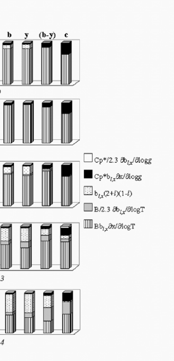
At first sight these large inconsistencies in the derivatives and in the limb darkening integrals and their derivatives seem to introduce large uncertainties in equation (1), but the situation is improved when we realize the different contributions from different terms in that equation. In Fig 11 I show these different contributions for a typical Scuti regime: ( K, ), and with a mean value for the adiabaticity parameter, i.e. =0.5. The different filters and filter combinations are the classical ones for the Strömgren photometric system, i.e. as a temperature indicator and as a luminosity indicator (at least for stars close enough to the Main Sequence).
As expected, the main contribution to any band and -value comes from temperature variations. Geometry variations, given by the term defined in (4), is the second important parameter for low -values but for =3 and 4 can become as large as, or even larger than, the temperature term defined in (2). It is also to be noted the large effect of the gravity variations in the color index , as properly defined by the Strömgren photometry. The basic idea is to use the geometry dependence, through the term defined in (4), for =0, 1 and 2 because of the changing sign of this term when passing from =0 to =2 and the null contribution for =1. So the main utility is not basically changed by the uncertainties of the other terms in equation (1) so allowing, for the lowest -values, a proper discrimination as we will see later on. In any case the term defined by (6) is always very small and the term defined by (3), no very well known neither, is only important for =4 when the smearing out effects along the stellar surface make the photometric method inapplicable.
4. “Regions of interest”
Once , derivatives and limb darkening have been calculated for a given star two unknown quantities in equation (1), , still remain in order to obtain the quantity we are looking for: , the degree of the spherical surface harmonic. is not a very well known quantity but it can be estimated from simultaneous photometric and radial velocities observations. Typical values for some Scuti given in Breger et al. (1976) range from to but phase lags for Dor stars are completely unknown. On the other hand the adiabaticity parameter can not be known from pure observations and one must assume some reasonable value for it which, according to equation (11), is restricted to values between 0 and 1.
In what follows I will adopt a constant value of 1.4 for and 5/3 for , which represent very well the Scuti regime.
When a range for the phase lag and for is assumed a diagram such as that shown in Fig 12 can be drawn, where amplitude ratios and phase differences are calculated for the range and and for the discriminant color pairs formed by and bands. In this review I will give the most usual combination of a visual band, , and a temperature indicator, , but other combinations are also useful, e.g. and as shown in Garrido et al. (1990). Uncertainties on the borders of these zones can be of the order of because of the actual precision of model atmospheres previously discussed. As can be seen in Fig 12 and originally demonstrated by Stamford and Watson (1981), the regions of radial modes are clearly separated from the regions of non-radial ones which in turn can be even distinguished among them. The reason is that, in the Scuti regime, where the phase lags are close to , a clear phase shift is originated for different photometric bands for the lowest -values, as previously discussed. For =3 the amplitude ratio is very different from the other three -values and this can be used to discriminate it. These phase differences are however very small and we need a very high precision photometry when determining phases and amplitudes from a classical Fourier fitting to the time series. On the other hand we do not know the phase lags for the Dor stars and hence these diagrams are not very useful for them until reliable values for these stars are known. At the end of this review I will give a explanation on how to calculate and values from multi-band photometric observations and we will see that the values deduced for the phase lags for these variables are close to .
The effect of using different model atmospheres is not relevant, discrimination is also attained in a clear way and the only remarkable difference is the location of the photometric temperature indicator , indicating a slight different temperature calibration for these two model atmospheres.


However the effect of the pulsation constant, is dramatic. When this value is lowered to a value of 0.015 days, corresponding to a radial 3rd or 4th overtone, then negative values are predicted also for radial modes and it is not true anymore that any negative value, in a vs. plot, corresponds to a non-radial mode. An example is given in Fig 13.
When we go to higher temperatures the radial regions at positive phase differences begin to shrink and finally disappear at around 8500 K even for a radial value for . An intermediate case is plotted in Fig 14 where the temperature is 8000 K and a higher radial value is assumed for . Notice the difference in amplitude ratios with respect to previous figures for the case =3 which could be due to the effect of the temperature derivatives in the model atmospheres.

In conclusion, these “regions of interest” are very dependent on the chosen photometric bands and used model atmospheres. In particular, model atmospheres with smoother derivatives and without discontinuities are required. A good test for these model atmospheres would be to compare the observed photometric variations with theoretical variations induced by a change in temperature. In other words not only to use standard stars for calibrating photometric indices but to use pulsating stars, with the above explained cautions, as standard stars regarding photometric variations.
-values deduced from these considerations should be taken with caution given the errors of the photometric measurements and the inconsistencies of model atmospheres. However there is a way to alleviate this problem: to know the quantities and the to solve equation (1) for .
5. Practical calculation of
I review in this section the two different methods to calculate actual values for the unknown quantities : A theoretical one given recently by Balona and Evers (1999) and another observational one given in Garrido et al. (1990).
5.1. Theoretical approach
Balona and Evers (1999) derive, from theoretical considerations, the unknown quantities . Although they use instead of those parameters are related through the equation:
| (15) |
Unfortunately these parameters are very sensible to the treatment of the convection specially for cool Scuti models, as shown by the authors in their Fig 3. The onset of the convection occurs at K; for higher temperatures the models are radiative and are constant and independent of the mixing length parameter adopted.
The authors develop a procedure which minimizes the distance between the observed and theoretically predicted color phases and amplitudes. These theoretical predictions come from non-adiabatic pulsation calculations of the couple from a model which also predicts the observed frequency of the pulsating star. They give some identification for the best observed stars in the Strömgren multicolor photometric system in their Table 4.
They apply the method to three double mode Scuti stars with period ratios typical of radial pulsators, i.e. AE UMa: 0.773, BP Peg: 0.772 and RV Ari: 0.773, and they find good solutions in general but they note that discrimination between =0 and =1 is sometimes poor. For some other HADS they find no solutions and for another they have to select a -mode as the best solution. The method can be limited by our ignorance of the convection but in principle could be very useful for radiative models, i.e. the hot regime of the Scuti stars.
5.2. Observational approach
This method was developed by Garrido et al. (1990) and uses multicolor photometry to derive the three unknown parameters and in equation (1).
At first sight a direct fitting to the formula appears to give very unstable values since its complexity prevents an inverse solution but, as indicated in that paper, if we assume no dependence on for the limb darkening integrals, which is nearly true for the lowest -values (see Fig 5, 6, 7 and 8), equation (1) becomes reversible for any -value. Errors are of the order of for =1, for =2, for =3 and for =4. In particular we need at least three bands, in order to have at least two color indices, but in practice we have the four Strömgren bands so allowing to calculate 15 different values for the couple .
Couples of values for are plotted in Fig 15, for the Scuti stars, where the error bars refers to 1-sigma value for the 15 values calculated for each star of Table 1. Errors bars for the other values not plotted in Fig 15 are of the same order and are not shown for clarity. All the values fall in the range of , which is just the expected range from theoretical arguments given before. Also as indicated by the existing simultaneous radial velocity observations. Values based on Kurucz models are more concentrated than values for the S&K models and the reason is not clear. In order to see the effect of the large variations shown by the derivatives in Fig 2, 3 and 4 I plot in them an average of these derivatives over temperature and gravity. The result is a more concentrated range for the values, so indicating that the dispersion shown by the derivatives could be a source of noise for calculating these parameters, because of the non-smoothness of model atmospheres.


![[Uncaptioned image]](/html/astro-ph/0001064/assets/x17.png)
![[Uncaptioned image]](/html/astro-ph/0001064/assets/x18.png)
In Fig 16 the couples are plotted for the Dor stars. These values are more spread basically for two reason: the small amplitude of the variations for these stars and the small phase differences observed for the photometric indices. Some physical unfounded values, i.e. greater than unity, appear for some stars. In any case the values derived using the Kurucz models show larger dispersions. This fact seems to indicate that Kurucz models are less stable for lower temperatures, since Dor stars are cooler than the majority of the Scuti stars. This fact could be also the explanation of the more concentrated values found before for Scuti stars. In any case the phase differences observed in the Strömgren bands for these stars seem to indicate that phase lags for these stars are close to zero. This is the first time that these values are calculated for these stars and, if confirmed, could be an important clue to determine the pulsational characteristics of these not very well understood variables. It is to be noted here that for an adiabatic atmosphere and that for a stellar spot!
6. Some examples of practical identifications
6.1. Scuti stars
The next step following the flow chart of Fig 1 is to calculate, from equation (1) and with known phase lags and known, the -value which minimizes the distances from the predicted values to the observed ones in all the photometric bands. To do that I have considered phases and amplitudes separately.
The best fit, in the sense of minimum variance for amplitudes, is marked “Amplitude variance” in the plots 17, 18, 19 and 10 and the corresponding to the phases, is marked “Phase variance”. The reason is that when looking at the “regions of interest” there are some -values which are separated in the phase difference axis, like =0 and 1 in Fig 12 and other are separated in the amplitude ratio axis, like =3.
As already mentioned the best way to test these identifications is to apply the method to the well known double mode Scuti stars which are oscillating into two radial modes. In Fig 17 I plot the results for these stars for the first four -values and for the two comparison axis: amplitudes and phases. As can be seen all the minima, both for fundamental and overtone modes, in the “phase variance” panels, are located always and in a very clear manner, except maybe for the first overtone of BP Peg, in the =0 position as expected from its radial nature. However the minima regarding “amplitude variance” are not very different for the first =0, 1, 2 values reflecting the behavior seen in Fig 12, in the sense that phases are discriminant in this regime for the lowest -values and amplitudes are for the higher ones. A blind application of the method for phases and amplitudes together could introduce then some extra variance which could change the minimum. It is important to know, before doing these comparisons, where the star regime falls in the phase difference vs amplitude ratio diagram.
When the method is applied to HADS the results are clear: all of them are pulsating in a radial mode (Fig 18).
![[Uncaptioned image]](/html/astro-ph/0001064/assets/x19.png)
![[Uncaptioned image]](/html/astro-ph/0001064/assets/x20.png)
Nevertheless when applied to the low amplitude Scuti stars the results are less conclusive because of the small amplitudes and the corresponding larger relative errors in the determination of amplitudes and especially phases. The results for the three best studied stars (due to their monoperiodicity) plotted seem to indicate that at least 20 CVn is oscillating in a radial mode, but the other two seem to be pulsating in an =1 or 2 mode (Fig 19).

6.2. Doradus stars
The results for the Dor stars, as indicated in Fig 20, show that all frequencies for all stars seem to be =1 non-radial modes if we accept the “phase variance” indications, whereas the discrimination is not so clear for the “amplitude variance” plots, indicating in this case the presence of modes with =1, 2 but not certainly 3. As explained in the previous section it would be convenient, in order to select the most relevant discriminator, to construct a “region of interest” for these variables with the new phase lag derived before. Such a plot is shown in Fig 21, where the relevant zones have been calculated for phase lags close to zero and atmospheric characteristics different to those of a Scuti star plus a very different pulsation constant which for a Dor star is an order of magnitude larger. It is clear from that figure that discrimination between =1 and =2 modes is based on phase differences and they are not distinguishable from amplitude ratios; =3 is however well discriminated from the other two lower -values. Going back to the interpretation of the results shown in Fig 20 for Dor stars, it becomes clear from the amplitude diagrams that these stars are not oscillating in an =3 mode and, from the phase diagrams, that they are probably oscillating in an =1 mode. However the small amplitudes and small phase differences observed in these stars prevent me to be sure about these conclusions. It would be very interesting to perform simultaneous photometry and spectroscopy for these objects in order to have real measurements of their phase lags.


7. Color information in space missions
The motivation to do asteroseismology from space is to detect and analyze solar like oscillations and to learn about the stellar interiors in other stars than the Sun. Color informations for these observations are not relevant since the modes can be easily identified from the rotational splitting. Due to the extremely small amplitudes expected to be measured, the number of photons is a crucial quantity in order to decrease the noise and therefore white light is the preferred solution. Modal identification is made by direct measuring of the rotational splitting. However it was previously demonstrated that multicolor information is essential to identify the modes for the stars we are interested in this conference, i.e. Scuti and Dor variables. Asteroseismological techniques become therefore possible opening the possibility to test stellar interiors in this region of the HR diagram.
COROT (http://www.astrsp-mrs.fr/www/ecorot.html) is a French asteroseismological and planet detection space mission which is now under study by the CNES. The scientific mission is explained in another part of this meeting. Basically there are two CCDs in the focal plane, one of them dedicated to asteroseismology, mainly for solar like oscillations, with no color information, and the other dedicated to planet detection by transit with color information in order to distinguish transits from other active phenomena in stars. This color information is achieved through the interposition of a prism in front of the CCD. The idea is to download two or three parts of this spectrum so giving different photometric colors. The field will contain several thousands of stars in order to be able to detect some events due to terrestrial planet transits during the two years for which the mission is expected to be operative.
MONS is mission lead by the Danish community which is also under study and will probably offer some color information. The reader is referred to another part of this meeting. Although the mission is not yet decided, it would probably have a dichroic prism in order to measure simultaneously two colors.
In any case these missions will provide data with very high precision and then much of the problems we have now for extracting information from photometry probably will disappear. We will be able to get data for multiperiodic Scuti stars and also for Dor with large enough amplitude to make feasible the photometric techniques that I review in this report.
I have made some simulations, constructing an arbitrary 12 color photometric system, for these two kind of pulsating stars in order to see the order of magnitude of the phases differences and amplitude ratios among the different photometric bands. These bands have arbitrarily 100 Å width distributed over the visible spectrum each 300 Å. I present the results in Fig 22 for a Scuti regime and in Fig 23 for a Dor regime. As shown there the main discriminant factor for radial and non-radial modes in Scuti stars is the phase difference between two colors, being also possible, depending on the precision, to discriminate among the non-radial modes. The main contribution of the amplitude ratios is to separate the high order =4 mode from the others. In any case a combination of the two diagrams will provide, at the precision we need, a clear identification for the lowest -values in the sense that the larger the difference in wavelength the better the discrimination, at least up to 3700 Å.

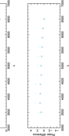
For Dor stars the situation is slightly different mainly due the the very high pulsation constant and the very different phase lag. As shown before the amplitude ratios do not separate =1 from =2 but the other non-radial modes are more clearly discriminated. The same is true for =2 and =3 concerning phase differences but fortunately the other modes can be separated. The combined information from the two panels could be of capital importance to separate modes.
With the precision we expect to have in COROT, from 100 to 10 ppm depending on the magnitude in the exoplanet focal plane, I estimate here phases and amplitudes will be so small that the method described becomes realistically applicable. I think that under these conditions an asteroseismological study of these variables is possible without the ambiguities of miss-identifications of the modes.
8. Conclusions
We already know that simple matching of observed to theoretically calculated frequency spectra for the best observed Scuti variables, such as FG Vir in Breger et al. (1999), do not give a unique solution. Possible combinations varying some physical inputs of the static models do not allow us to constraint the theoretical model. An identification procedure is then required for the observed modes.
We have seen that the success of the photometric method to identify the degree of the spherical harmonic for Scuti and Dor stars depends on the model atmospheres we are using and on the precision on the photometric data we are analysing.
Although the global uncertainties bound to the photometric calibrations, i.e. calculation of and, do not affect dramatically to the discrimination procedure, the model atmospheres present some subtle characteristics. Kurucz models present some inconsistencies, at the level of the required continuities in the fluxes and derivatives which, in the HR region where the stars we are investigating fall, seem to be related with the treatment of convection and in particular of overshooting. Other improved models, such as those described in Smalley and Kupka (1997), present a smoother behavior at these temperatures and gravities but some inconsistencies still remain regarding continuities in the flux derivatives. An appropriate comparison with very accurate photometric data on the variables could be useful to improve these discontinuities in the models.
Photometric precision is now sufficient only for the highest amplitude pulsating variables. In particular, nowadays existing HADS photometric data with precisions of around 1 mmag, are useful to identify their oscillation modes. From observations of other variables with lower amplitudes I estimate that we need at least signal to noise ratios of the order of 20–30 in order to have a stable Fourier solution and then make the photometric method feasible.
The method supplies reasonable -values for HADS, i.e. all of them are found to be radial pulsators, and for some other Scuti stars with lower amplitudes non-radial modes seem to be identified. In any case when applied to known radial pulsators, as the double mode Scuti stars, the results are consistent with their radial nature.
When applied to the new discovered Dor stars the method is able to give estimations of two not very well known physical quantities, and . The phase lags for these stars, if confirmed, would be very different from the classical value observed in Scuti stars. Furthermore the existing multi-band photometry for some of them seems to indicate that these stars are very probably oscillating in an =1 mode.
It is also shown that, within the uncertainties, the method provides estimations of which can be used to compare with theoretical models. These quantities depend very much on the convection parameters which are not very well known and could be useful to modelize the convection in these stars, which in turn could give important clues to the understanding of the onset of the convection in this region of the HR diagram.
The new generation of asteroseismological space missions will provide in a next future a huge quantity of very high quality data for these stars. As demonstrated in this review and in order to understand and disentangle the complicated frequency spectrum of multiperiodic Scuti stars we need colored information as demonstrated in this review.
Actual model atmospheres need to be improved, specially the smoothness in the derivatives and limb darkening variations, in order to extract the whole potential of the photometric discrimination method.
Acknowledgments.
I am very grateful to Enrique Solano for supplying me the Kurucz fluxes and limb darkening coefficients and to Antonio Claret for the PHOENIX limb darkening coefficients. I am also grateful to Chris Sterken for many helpful comments, and to the editors for making possible a more readable version of the manuscript.
References
Balona, L. A. and Stobie, R. S. 1979a, MNRAS, 189, 627
Balona, L. A. and Stobie, R. S. 1979b, MNRAS, 189, 649
Balona, L. A. and Evers, E. A. 1999, MNRAS, 302, 349
Breger, M. et al. 1993, A&A, 271, 482
Breger et al. 1976, ApJ, 210, 163
Breger, M. et al. 1999, A&A, 341, 151
Canuto, V. M. and Mazzitelli, I. 1991, ApJ, 370, 295
Canuto, V. M. and Mazzitelli, I. 1992, ApJ, 389, 724
Dziembowski, W. 1977, Acta Astronomica, 27, 203
Garrido, R. et al. 1990, A&A, 234, 262
Frandsen, S. et al. 1996, A&A, 308, 132
Hauschildt, P. H. 1992, J. Quant. Spectrosc. Radiat. Transfer, 47, 433
Hauschildt, P. H. 1993, J. Quant. Spectrosc. Radiat. Transfer, 50, 301
Hauschildt, P. H. and Baron, E. 1995, J. Quant. Spectrosc. Radiat. Transfer, 54, 987
Hauschildt et al. 1996, ApJ, 462, 386
Hayes, D. S. 1985, ApJ, 289, 726
Hayes, D. S. and Latham, D. W. 1975, ApJ, 197, 593
Hintz, E. G. et al. 1998, PASP, 110, 689
Kurucz, R. L. 1993, Kurucz CD-ROM 13:ATLAS9, SAO, Cambridge, USA
Pamyatnykh, A. A. et al. 1998, A&A, 331, 141
Rodriguez, E. et al. 1988a, Rev. Mex. Astron. Astrofis., 16, 7
Rodriguez, E. et al. 1989, Thesis, Univ. Granada
Rodriguez, E. et al. 1990, Rev. Mex. Astron. Astrofis., 20, 37
Rodriguez, E. et al. 1992a, A&AS, 93, 189
Rodriguez, E. et al. 1992b, A&AS, 96, 429
Rodriguez, E. et al. 1993a, A&A, 273, 473
Rodriguez, E. et al. 1993b, A&AS, 100, 571
Rodriguez, E. et al. 1993c, A&AS, 101, 421
Rodriguez, E. et al. 1994, A&AS, 106, 21
Rodriguez, E. et al. 1995, MNRAS, 277, 965
Rodriguez, E. et al. 1998, A&A, 331, 171
Rolland, A. et al. 1991, A&AS, 91, 347
Smalley, B. and Kupka, F. 1997, A&A, 328, 349
Smalley, B. 1993, A&A, 274, 391
Stamford, P. A. and Watson, R.D. 1981, Ap&SS, 77, 131
Watson, R. D. 1988, Ap&SS, 140, 225