Eccentric stellar discs with strong density cusps and separable potentials

Abstract

We introduce a class of eccentric discs with “strong” density cusps whose potentials are of Stäckel form in elliptic coordinates. Our models exhibit some striking features: sufficiently close to the location of the cusp, the potential and surface density distribution diverge as $\Phi\propto r^{-1}$ and $\Sigma\propto r^{-2}$, respectively. As we move outward from the centre, the model takes a non-axisymmetric, lopsided structure. In the limit, when $r$ tends to infinity, the isocontours of $\Phi$ and $\Sigma$ become spherically symmetric. It is shown that the configuration space is occupied by three families of regular orbits: eccentric butterfly, aligned loop and horseshoe orbits. These orbits are properly aligned with the surface density distribution and can be used to construct self-consistent equilibrium states.

1 INTRODUCTION

High resolution observations based on Hubble Space Telescope photometry of nearby galaxies have increased our understanding of the central regions of elliptical and spiral galaxies. It was found that in most galaxies density diverges toward the centre in a power-law cusp. In the presence of a cusp, regular box orbits are destroyed and replaced by chaotic orbits (Gerhard & Binney 1985). Through a fast mixing phenomenon, stochastic orbits cause the orbital structure to become axisymmetric at least near the centre (Merritt & Valluri 1996). These results are confirmed by the findings of Zhao et al. (1999, hereafter Z99). Their study reveals that highly non-axisymmetric, scale-free mass models can not be constructed self-consistently. Among the models studied for self-consistency, one can refer to the integrable, cuspy models of Sridhar & Touma (1997, hereafter ST97). Without a nuclear black hole (BH), centrophobic bananas are the only family of orbits presenting in ST97 discs. Although such orbits elongate in the same direction as density profile, the orbital angular momentum takes a local minimum somewhere rather than the major axis where the surface density has a maximum. This is the main obstacle for building self-consistent equilibria by regular bananas (Syer & Zhao 1998; Z99). A similar situation occurs for anti-aligned tube and high resonance orbits for which one could not be able to fit the curvatures of orbits and surface density distribution near the major axis (Z99). According to the results of Miralda-Escudé & Schwarzschild (1989), it is only possible to construct self-consistent models by certain families of fish orbits.

The orbital structure of stellar systems is enhanced by central BHs in a different manner. Although nuclear BHs destroy box orbits, they enforce some degree of regularity in both centred and eccentric discs (Sridhar & Touma 1999, hereafter ST99). In systems with analytical cores and central BHs, a family of long-axis tube orbits can help the host galaxy to maintain its non-axisymmetric structure within the BH sphere of influence (Jalali 1999).

In this paper, we present a class of non-scale-free, lopsided discs, which display a collection of properties expected in self-consistent non-axisymmetric cuspy systems. Our models are of Stäckel form in elliptic coordinates (e.g., Binney & Tremaine 1987) for which the Hamilton-Jacobi equation separates and stellar orbits are regular. In central regions where the effect of the cusp dominates, the potential functions of our distributed mass models are proportional to $r^{-1}$ as $r\rightarrow 0$. So, we attain an axisymmetric structure near the centre which is consistent with the predicted nature of density cusps. The slope of potential function changes sign as we depart from the centre and our model galaxies considerably become non-axisymmetric. Non-axisymmetric structure is supported by a family of eccentric loop orbits, which are aligned with the lopsidedness. Our potential functions have a local minimum around of which a family of eccentric butterfly orbits emerges. Close to the centre, loop orbits break down and give birth to a new family of orbits, horseshoe orbits. Stars moving in horseshoes lose their kinetic energy as they approach to the centre and contribute a large amount of mass to form a cusp. Our models can be applied to the study of dynamics in systems with double nucleus such as M31 (Tremaine 1995, hereafter T95) and NGC4486B (Lauer et al. 1996).

2 THE MODEL

Consider the Hamiltonian function

$${\cal H}=\frac{1}{2}(p_{x}^{2}+p_{y}^{2})+\Phi(x,y),$$ (1)

which is described in cartesian coordinates, $(x,y)$. The variables $p_{x}$ and $p_{y}$ denote the momenta conjugate to $x$ and $y$, respectively. $\Phi$ is the potential due to the self-gravity of the disc. Let us express ${\cal H}$ in elliptic coordinates, $(u,v)$, through the following transformations

$$x = a(1+\cosh u\cos v),$$ (2)

$$y = a\sinh u\sin v,$$ (3)

$$u \geq 0,~{}~{}0\leq v\leq 2\pi,$$

where $a$ is constant and $2a$ is the distance between the foci of confocal ellipses and hyperbolas defined by the curves of constant $u$ and $v$, respectively. In the new coordinates, the Hamiltonian function becomes

$${\cal H}=\frac{1}{2a^{2}(\sinh^{2}u+\sin^{2}v)}(p_{u}^{2}+p_{v}^{2})+\Phi(u,v),$$ (4)

with $p_{u}$ and $p_{v}$ being the new canonical momenta. We think of those potentials which take Stäckel form in elliptic coordinates. The most general potential of Stäckel form is

$$\Phi(u,v)=\frac{F(u)+G(v)}{2a^{2}(\sinh^{2}u+\sin^{2}v)},$$ (5)

where $F$ and $G$ are arbitrary functions of their arguments. By this assumption, the Hamilton-Jacobi equation separates and results in the second integral of motion, $I_{2}$. We get

$$I_{2}=p_{u}^{2}-2a^{2}E\sinh^{2}u+F(u),$$ (6)

or equivalently

$$-I_{2}=p_{v}^{2}-2a^{2}E\sin^{2}v+G(v),$$ (7)

where $E$ is the total energy of the system, $E\equiv{\cal H}$.

We now introduce a class of potentials with

$$F(u) = C(\cosh u)^{\gamma},$$

$$G(v) = -C\cos v|\cos v|^{\gamma-1},$$ (8)

where $C>0$ and $\gamma$ are constant parameters. One can readily verify that

$$\cosh u=\frac{1}{2a}(r+s),~{}~{}\cos v=\frac{1}{2a}(r-s),$$ (9)

where

$$r^{2}=x^{2}+y^{2},~{}~{}s^{2}=(x-2a)^{2}+y^{2}.$$ (10)

We substitute from (10) into (8) and express $\Phi$ in the $(x,y)$ coordinates:

$$\Phi = K\frac{(r+s)^{\gamma}-(r-s)|r-s|^{\gamma-1}}{2rs},$$ (11)

$$K = C(2a)^{-\gamma}.$$

The surface density distribution, associated with $\Phi$, is determined as (see Binney & Tremaine 1987):

$$\Sigma(x^{\prime},y^{\prime})=\frac{1}{4\pi^{2}G}\int\int\frac{(\nabla^{2}\Phi)dxdy}{\sqrt{(x^{\prime}-x)^{2}+(y^{\prime}-y)^{2}}}.$$ (12)

We examine the characteristics of the potential and surface density functions for small and large radii. Very close to the centre, we have $r\ll s$ that simplifies (11) as follows

$$\Phi=\frac{Ks^{\gamma-1}}{2}\frac{(1+\frac{r}{s})^{\gamma}+(1-\frac{r}{s})^{\gamma}}{r}.$$ (13)

One can expand $(1+\frac{r}{s})^{\gamma}$ and $(1-\frac{r}{s})^{\gamma}$ in terms of $r/s$ to obtain

$$\Phi=\frac{Ks^{\gamma-1}}{r}\left[1+\sum_{n=1}^{\infty}\frac{\Gamma(\gamma+1)}{(2n)!\Gamma(\gamma-2n+1)}\left(\frac{r}{s}\right)^{2n}\right],$$ (14)

where $\Gamma$ is the well known Gamma function. As $r$ tends to zero, $s$ is approximated by $2a$ and $r/s\rightarrow 0$. Therefore, Equation (14) reads

$$\Phi\approx\frac{K(2a)^{\gamma-1}}{r}.$$ (15)

Dimensional considerations show that the surface density $\Sigma$ will approximately be proportional to $r^{-2}$. Thus, sufficiently close to the centre, we obtain a strong density cusp with spherical symmetry. When $r$ tends to infinity, the potential $\Phi$ is approximated as

$$\Phi\approx K2^{\gamma-1}r^{\gamma-2}.$$ (16)

So, we find out

$$\Sigma\propto r^{\gamma-3}.$$ (17)

We have to select those values of $\gamma$ for which the surface density distribution is plausible and orbits are bounded. According to (17), the surface density decays outward ($r\rightarrow\infty$) for $\gamma<3$. Moreover, Equation (16) shows that orbits will be escaping if $\gamma\leq 2$. To verify this, consider the force exerted on a star, which is equal to $-\nabla\Phi$. This force will always be directed outward for $\gamma\leq 2$ and results in escaping motions. Therefore, we are confined to $2<\gamma<3$.

(a)

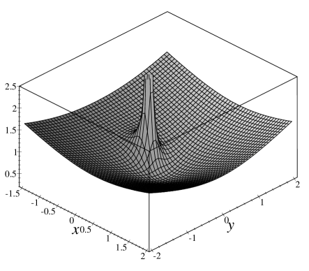
(b)

Figure 1: As a demonstrating example, we have determined the potential $\Phi$ for $\gamma=2.8$, $a=0.5$ and $K=0.2$. Figures (a) and (b) show the isocontours and a three dimensional view of $\Phi$, respectively.

We have used Equations (11) and (12) to compute $\Phi$ (Figure 1) and $\Sigma$ (Figure 2) for $\gamma=2.8$. Due to the complexity of $\nabla^{2}\Phi$, we have utilized a numerical scheme to evaluate the double integral of (12). The potential and surface density functions are symmetric with respect to the $x$-axis and are cuspy at $(x=0,y=0)$. The potential $\Phi$ has a local minimum at $(x=a,y=0)$ that plays an important role in the evolution of orbits. This minimum point has no image in the plane of the surface density isocontours. The surface density monotonically decreases outward from the centre. As it is evident from Figure 2, a non-axisymmetric, lopsided structure is present at moderate distances from the centre.

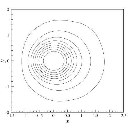
Figure 2: The surface density isocontours corresponding to the potential function of Figure 1.

3 ORBITS

To this end, we classify orbit families. Having the two isolating integrals $E$ and $I_{2}$, one can find the possible regions of motion by employing the positiveness of $p_{u}^{2}$ and $p_{v}^{2}$ in (6) and (7). We define the following functions:

$$f(u) = -2a^{2}E\sinh^{2}u+F(u),$$ (18)

$$g(v) = -2a^{2}E\sin^{2}v+G(v),$$ (19)

where $F(u)$ and $G(v)$ are given as (8). By virtue of $p_{u}^{2}\geq 0$ and $p_{v}^{2}\geq 0$ one can write

$$I_{2}-f(u) \geq 0,$$ (20)

$$-I_{2}-g(v) \geq 0.$$ (21)

Due to the nature of $\Phi$, no motion exists for negative energies. Hence, $E$ can only take positive values, $E>0$. Our classification is based on the behavior of $f(u)$ and $g(v)$. The most general form of $f(u)$ is attained for $\gamma C<4a^{2}E$. In such a circumstance, $f(u)$ takes a local maximum at $u=0$, $f_{\rm M}=f(0)=C$, and a global minimum at $u=u_{\rm m}$, $f_{\rm m}=f(u_{\rm m})$, where

$$\cosh u_{\rm m}=\left(\frac{4a^{2}E}{C\gamma}\right)^{\frac{1}{\gamma-2}},$$ (22)

and

$$f_{\rm m}=-2a^{2}E\sinh^{2}u_{\rm m}+C(\cosh u_{\rm m})^{\gamma}.$$ (23)

According to (20) we obtain

$$I_{2}\geq f_{\rm m}.$$ (24)

On the other hand, $g(v)$ has a global maximum at $v=\pi$, $g_{\rm M}=g(\pi)=C$, and two global minima at $v=\pi/2$ and $v=3\pi/2$, $g_{\rm m}$=$g(\pi/2)$=$g(3\pi/2)$=$-2a^{2}E$. Therefore, Inequality (21) implies

$$I_{2}\leq 2a^{2}E.$$ (25)

By combining (24) and (25) one achieves

$$f_{\rm m}\leq I_{2}\leq 2a^{2}E.$$ (26)

It should be noted that $2a^{2}E>C$. This is because of $2<\gamma<3$. $f_{\rm m}$ and in consequence $I_{2}$, can take both positive and negative values. Depending on the value of $I_{2}$, three general types of orbits are generated:

(i) Eccentric Butterflies. For $C<I_{2}<2a^{2}E$, the allowed values for $u$ and $v$ are

$$u\leq u_{0},~{}v_{b,1}\leq v\leq v_{b,2},~{}v_{b,3}\leq v\leq v_{b,4},$$ (27)

where $u_{0}$ and $v_{b,i}$ ($i=1,2,3,4$) are the roots of $f(u)=I_{2}$ and $g(v)=-I_{2}$, respectively. As Figure 3a shows, the horizontal line that indicates the level of $I_{2}$, intersects the graph of $f(u)$ at one point, which specifies the value of $u_{0}$. The line corresponding to the level of $-I_{2}$ intersects $g(v)$ at four points that give the values of $v_{b,i}$s (Figure 3b). In this case the motion takes place in a region bounded by the coordinate curves $u=u_{0}$ and $v=v_{b,i}$. The orbits fill the shaded region of Figure 4a. These are butterfly orbits (de Zeeuw 1985) displaced from the centre. We call them eccentric butterfly orbits.

                  $(a)$ $(b)$

                  $(c)$ $(d)$

                  $(e)$ $(f)$

Figure 3: The graphs of $f(u)$ and $g(v)$ for $\gamma=2.8$, $C=0.2$, $E=1.2$ and $a=0.5$. The horizontal lines indicate the levels of $I_{2}$ and $-I_{2}$ in the graphs of $f(u)$ and $g(v)$, respectively. (a) $I_{2}=0.4$ (b) $-I_{2}=-0.4$ (c) $I_{2}=-0.25$ (d) $-I_{2}=0.25$ (e) $I_{2}=-0.1$ (f) $-I_{2}=0.1$.

(ii) Aligned Loops. We now let $I_{2}$ be negative so that $f_{\rm m}<I_{2}<-C$. In this case the equation $f(u)=I_{2}$ has two roots, $u_{l,1}$ and $u_{l,2}$, which can be identified by the intersections of $f(u)$ and the level line of $I_{2}$ (see Figure 3c). The equation $g(v)=-I_{2}$ has no real roots and Inequality (21) is always satisfied (Figure 3d). The allowed ranges of $u$ and $v$ will be

$$u_{l,1}\leq u\leq u_{l,2},~{}~{}0\leq v\leq 2\pi.$$ (28)

The orbits fill a tubular region as shown in Figure 4b. These orbits are bound to the curves of $u=u_{l,1}$ and $u=u_{l,2}$ and elongate in the same direction as lopsidedness. Following ST99, they are called aligned loops.

(iii) Horseshoes. For $-C<I_{2}<C$, we have a different story. In this case, both of the equations $f(u)=I_{2}$ and $g(v)=-I_{2}$ have two roots. We denote these roots by $u=u_{h,i}$ and $v=v_{h,i}$ ($i=1,2$). In other words, the level lines of $\pm I_{2}$ intersect the graphs of $f(u)$ and $g(v)$ at two points as shown in Figures 3e and 3f. The orbits fill the shaded region of Figure 4c, which looks like a horseshoe. We call these horseshoe orbits. The orbital angular momentum of stars moving in horseshoes ($G=xp_{y}-yp_{x}$) flips sign when stars arrive at one of the coordinate curves $v=v_{h,1}$ or $v=v_{h,2}$.

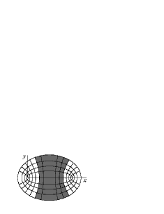
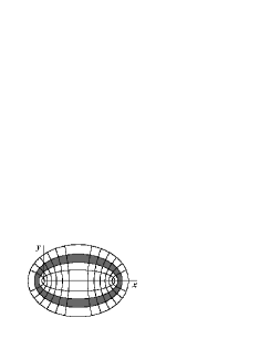
                 $(a)$ $(b)$

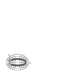
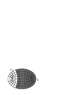
                 $(c)$ $(d)$

Figure 4: The possible families of orbits: (a) an eccentric butterfly orbit (b) an aligned loop orbit (c) a horseshoe orbit (d) a lens orbit associated with $I_{2}=C$.

For $\gamma C>4a^{2}E$, $f(u)$ is a monotonically increasing function of $u$ and eccentric butterflies are the only existing family of orbits. There are three transitional cases corresponding to $I_{2}=C$, $I_{2}=2a^{2}E$ and $I_{2}=f_{\rm m}$. For $I_{2}=C$, eccentric butterflies extend to a lens orbit as shown in Figure 4d. For $I_{2}=2a^{2}E$, stars undergo a rectilinear motion on the line $x=a$ with the amplitude of $\pm a\sinh u_{0}$ in the $y$-direction. For $I_{2}=f_{\rm m}$, loop orbits are squeezed to an elliptical orbit defined by $u=u_{\rm m}$.

4 DISCUSSIONS

In this work we explore a credible model based on the self-gravity of stellar discs to explain how an eccentric disc, with strong density cusp, can be in equilibrium. Our mass models exhibit most features of eccentric stellar systems, especially, double nucleus ones such as M31 and NGC4486B.

All of the orbits of our model discs are non-chaotic. Below, we clarify how the existing families of orbits help the eccentric disc to maintain the assumed structure.

The force exerted on a star is equal to $-\nabla\Phi$. The motion under the influence of this force can be tracked on the potential hill of Figure 1b. This helps us to better imagine the motion trajectories.

As Figure 1b shows, the potential function is concave. A test particle released from distant regions with $x>0$ and “small” initial velocity, slides down on the potential hill and moves toward the local minimum at ($x=a,y=0$). After passing through the neighborhood of this point (there are some trajectories that exactly visit the minimum point), the test particle climbs on the potential hill until its potential energy becomes maximum. Then, the particle begins to slip down again. This process is repeated and the trajectory of the particle fills an eccentric butterfly orbit. Stars moving in eccentric butterflies form a local group in the vicinity of ($x=a,y=0$). The accumulation of stars around this local minimum of $\Phi$ can create a second nucleus like P2 in M31 (see T95). The predicted second nucleus will approximately be located at the “centre” of loop orbits while the brighter nucleus (P1) is at the location of the cusp.

Aligned loop orbits occur when the orbital angular momentum is high enough to prevent the test particle to slide down on the potential hill. The boundaries of loop orbits are defined by the ellipses $u=u_{l,1}$ and $u=u_{l,2}$. The central cusp is located at one of the foci of these ellipses. Aligned loops have the same orientation as the surface density isocontours (compare Figures 2 and 4b). Thus, according to the results of Z99, it is possible to construct a self-consistent model using aligned loop orbits.

Similarly, we can describe the behavior of horseshoe orbits. Stars that start their motion sufficiently close to the centre, are repelled from the centre because the force vector is not directed inward in this region. As they move outward, their orbits are bent and cross the $x$-axis with non-zero angular momentum. These stars considerably lose their kinetic energy as they approach the centre (this is equivalent to their climb on the cuspy region of the potential hill). Meanwhile, the orbital angular momentum takes a minimum and switches sign somewhere on the boundary of horseshoe orbit. This boundary is defined by $v=v_{h,1}$ (or $v=v_{h,2}$) and can be chosen arbitrarily close to the centre. These stars spend much time near the centre and deposit a large amount of mass, which generates a cusp. Therefore, horseshoe orbits can be used to construct a self-consistent strong cusp. The method of Z99 is no longer applicable to horseshoes because such orbits don’t cross the long axis (here the $x$-axis) near the centre. In fact, horseshoe orbits are an especial class of boxlets that appropriately bend toward the centre. The lack of such a property in banana orbits causes the ST97 discs to be non-self-consistent.

In the case of M31 and NGC4486B, if we suppose that loop and high-energy butterfly orbits control the overall shape of outer regions, horseshoe orbits together with low-energy butterflies (small-amplitude liberations around the local minimum of $\Phi$) can support the existence and stability of a double nucleus. The parameter $a$ will indicate the distance between P1 and P2.

There remains an important question: what does happen to a star just at the centre? The centre of the model, where the cusp has been located, is inherently unstable. With a small disturbance, stars located at ($x=0,y=0$) are repelled from the centre. But, the time that they spend near the centre will be much longer than that of distant regions when they move in horseshoes. We remark that the stars of central regions live in horseshoe orbits. Although one can place a point mass (black hole) at the centre without altering the Stäckel nature of the potential, such a point mass will not remain in equilibrium and leaves the centre. Based on the results of this paper, we conjecture that there may not be any mass concentration just at the centre of cuspy galaxies. However, a very dense region exists arbitrarily close to the centre! This may be an explanation of dark objects at the centre of cuspy galaxies. The centre of our model galaxies is unreachable. Our next goal is to apply the method of Schwarzschild (1979,1993) for the investigation of self-consistency.

References

- [R1] Binney J., Tremaine S., 1987, Galactic Dynamics, Princeton University Press, Princeton
- [R2] de Zeeuw P.T., 1985, MNRAS, 216, 273
- [R3] Gerhard O.E., Binney J., 1985, MNRAS, 216, 467
- [R4] Jalali M.A., 1999, MNRAS, 310, 97
- [R5] Lauer T.R., et al., 1996, ApJ, 471, L79
- [R6] Merritt D., Quinlan G.D., 1998, ApJ, 498, 625
- [R7] Merritt D., Valluri M., 1996, ApJ, 471, 82
- [R8] Miralda-Escudé J., Schwarzschild M., 1989, ApJ, 339, 752
- [R9] Schwarzschild M., 1979, ApJ, 232, 236
- [R10] Schwarzschild M., 1993, ApJ, 409, 563
- [R11] Sridhar S., Touma J., 1997, MNRAS, 287, L1-L4 (ST97)
- [R12] Sridhar S., Touma J., 1999, MNRAS, 303, 483 (ST99)
- [R13] Syer D., Zhao H.S., 1998, MNRAS, 296, 407
- [R14] Tremaine S., 1995, AJ, 110, 628 (T95)
- [R15] Zhao H.S., Carollo C.M. & de Zeeuw P.T., 1999, MNRAS, 304, 457 (Z99)