Abstract

A large set of TREESPH simulations is used to test the global morphology of galaxy clusters and its evolution against X–ray data. A powerful method to investigate substructures in galaxy clusters are the power ratios introduced by Buote $\&$ Tsai. We consider three flat cosmological models: CDM, $\Lambda$CDM ($\Omega_{\Lambda}=0.7$) and CHDM ($\Omega_{h}=0.2$, 1 massive $\nu$), all normalized so to fit the observed number of clusters. For each model we built 40 clusters, using a TREESPH code, and performed a statistical comparison with a data sample including nearby clusters observed with ROSAT PSPC instrument. The comparison disfavors the $\Lambda$CDM model, as clusters appear too relaxed, while CDM and CHDM clusters, in which a higher degree of complexity occurs, seem to be closer to observations. A better fit of data can be expected for some different DM mix. If DM distributions are used instead of baryons, we find substructures more pronounced than in gas and models have a different score. Using hydrodynamical simulations is therefore essential to our aims.

Morphological evolution of X–ray clusters using hydrodynamical simulations”

¹SISSA Via Beirut 2-4, I34014, Trieste, Italy
²Istituto di Fisica Cosmica, CNR, via Bassini 15, I20133, Milano, Italy
³Dipartmento di Fisica dell’ Università di Milano-BICOCCA, Via Celoria 16, I20133, Milano, Italy
⁴INFN – Sezione di Milano, Italy

1 Introduction

Clusters of galaxies are likely to be dynamically young systems and a promising way to constrain cosmological models arises from the study their substructures ([9]; [1]).

Among the methods suggested to quantify the degree of inhomogeneity in clusters ([10]; [7]; [4] ), one of the most promising is based on the so-called power ratios $\Pi^{(m)}$ ([12], hereafter VGB99; [2]). It amounts to a multipole expansion accounting for the angle dependence of cluster X–ray surface brightness, limited to the first few multipole terms and at fixed scales (typically of the order of the Mpc). This is an effective and synthetic way to discriminate cluster features and $\Pi^{(m)}$ are found do depend on the cosmological model enabling to discriminate among different cosmologies.

2 Power ratios: definition and evolution

The number of photons collected by ROSAT PSPC does not depend on the temperature $T$, if it is$\lower 1.93748pt\hbox{$\;\buildrel>\over{\sim}\;$}1$ keV. We can then assume that the X–ray surface brightness $\Sigma_{X}=\Lambda\int{\rho_{b}^{2}({\bf r})dz}$. Here $\Lambda\sim const$ results from an integration along the line of sight.

The procedure to work out $\Pi^{(m)}$ is as follows (see, e.g., [5], hereafter G98; VGB99; [2]): (i) $\rho_{b}^{2}({\bf r})$ is projected along a line of sight on a (random) plane to yield the $X$–ray surface brightness $\Sigma(R,\varphi)$; the centroid is used as origin. (ii) By solving the Poisson equation $\nabla^{2}\Phi=\Sigma(R,\varphi)$ we obtain the pseudo–potential $\Phi(R,\varphi)$. (iii) The coefficients of the expansion of $\Phi$ in plane harmonics will be used to build the power ratios $\Pi^{(m)}(R_{ap})=\log_{10}(P_{m}/P_{0})$. Here, $P_{m}(R)=(\alpha_{m}^{2}+\beta_{m}^{2})/2m^{2}~{},P_{0}=[\alpha_{0}\ln(R/{\rm kpc})]^{2}$, while

$$\alpha_{m}=\int_{0}^{1}{ds\,s^{m+1}\int_{0}^{2\pi}{d\varphi[\Sigma(sR,\varphi)R^{2}]\cos(m\varphi)}},$$ (1)

and $\beta_{m}$ has an identical definition, with sin instead of cos. Owing to the definition of the centroid, $\Pi^{(1)}$ vanishes. We shall restrict our analysis to $\Pi^{(m)}$($m=2,3,4$), to account for substructures  on scales not much below $R$ itself. We consider three different aperture radii $R_{ap}=0.4,0.8,1.2h^{-1}$Mpc.

Because of its evolution, a cluster moves along a curve of the 3–dimensional space spanned by such $\Pi^{(m)}$’s; this curve is called evolutionary track. Quite in general, a cluster starts from a configuration away from the origin, corresponding to a large amount of internal structure and evolves towards isotropization and homogeneization.

Actual data, of course, do not follow the motion of a given cluster along the evolutionary track. Different clusters, however, lie at different redshifts and can be used to describe a succession of evolutionary stages.

3 The simulated and the observed cluster sample

We consider three spatially flat cosmological models: CDM, $\Lambda$CDM with a cosmological constant accounting for $70\%$ of the critical density, and CHDM with 1 massive neutrino with mass $m_{\nu}=4.65\,$eV, yielding a HDM density parameter $\Omega_{h}=0.20$. We set $h=0.5$ for CDM and CHDM and $h=0.7$ for $\Lambda$CDM; for all models the primeval spectral index $n=1$ and the baryon density parameter is selected to give $\Omega_{b}h^{2}=0.015$. All models were normalized in order to reproduce the present observed cluster abundance ([4], [6]).

In order to achieve a safe statistical basis for our analysis, for each cosmological model, we select the 40 most massive clusters from an N–body P3M simulation. For each of them, we perform a hydrodynamical TREESPH simulation (VGB99, G98; see also [8] and [11]).

Clusters are distributed in redshift so to reproduce the same redshfit distribution of the observed cluster sample.

Our observed data set is the same used by [3], including nearby ($z\lower 1.93748pt\hbox{$\;\buildrel<\over{\sim}\;$}0.2$) clusters observed with ROSAT PSPC instrument (see VGB99, G98 for details). The resulting sample is partially incomplete, but, clusters were not selected for reasons related to their morphology and the missing clusters are expected to have a distribution of power ratios similar to the observed one.

4 Results and Conclusions

For simulated clusters, power ratios $\Pi^{(m)}$ have been computed from the gas distribution.

A visual inspection of how the $\Pi^{(m)}$ are distributed can be obtained from Fig.1, whose histograms show the fraction of clusters with a given $\Pi^{(m)}$ . Here we show the distribution for $\Pi^{3}$ and $R_{ap}=0.8h^{-1}$Mpc for each cosmological model and for the ROSAT data sample; distributions for the other $\Pi^{(m)}$ and the other apertures show a similar behavior

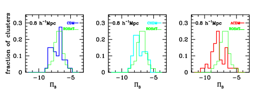
Figure 1: Histograms of $\Pi^{3}$ in the $R_{ap}=0.8h^{-1}$Mpc for simulated clusters.

Quite in general we can conclude that while CDM and CHDM  are marginally consistent with data, $\Lambda$CDM  is far below them. In order to quantify these differences, we used the Student t–test, the F–test and the Kolgomorov–Smirnov (KS) test. For example, according to the t–test, the probability $p$–$t$ that the simulated and observed power ratios distributions are originated from the same process is roughly in the ranges 0.11–0.60 for CDM, 0.03–0.37 for CHDMand 0.15$\cdot 10^{-4}$–0.87$\cdot 10^{-2}$ for $\Lambda$CDM. The other statistical tests provide similar probabilities. Such figures seem to exclude that $\Lambda$CDM can be considered a reasonable approximation to data. The best score belongs to CDM, but also CHDM is not fully excluded and different mixtures could certainly have better performance. An inspection of the model clusters actually shows that the $\Lambda$CDM  model does produce less substructures than the other models do. A possible interpretation of such output is that the actual amount of substructures is governed by $\Omega_{0}$ rather than by the shape of power spectra.

According to the same tests, if cosmological models are compared with data on the basis of DM $\Pi^{(m)}$, values are shifted, indicating an increase in the amount of substructures for DM with respect to the gas. This is to be ascribed to the smoothing effects of the interactions among gas particles, which erase anisotropies and structures, while DM $\Pi^{(m)}$scarcely feel dissipative processes. Hence, using DM $\Pi^{(m)}$leads to biased scores: CDM and CHDM models keep too many substructures and are no longer consistent with data; on the contrary, the increase of substructures pushes $\Lambda$CDM to agree with ROSAT sample outputs.

We also considered the cluster distribution in the 3–dimensional parameter space with axes given by $\Pi^{(m)}$ ($m=2,3,4$), as well as projections of such distributions on planes. Comparing such distributions for data and models, we find a significantly stronger correlation of $\Pi^{(m)}$ in models than in data. Distributions for simulated clusters show a linear trend while distributions of observed clusters tend to be more scattered than simulated points. The degree of correlation depends on the model, but seems however in disagreement with data. Model clusters tend to indicate a significantly faster evolution than data. The cosmological model which seems closest to data is CHDM and it is possible that different CHDM mixtures can lead to further improvements. Also $\Lambda$ models with $\Omega_{m}>0.5$ might deserve to be explored. Virialized clusters had their turn–around at a time $<t_{o}/3$ ($t_{o}$: present age of the Universe). In turn, $\Omega_{\Lambda}$ becomes dominant at $z=(\Omega_{\Lambda}/\Omega_{m})^{1/3}$. If such redshift occurs at a time $\sim t_{o}/3$, we expect results from $\Lambda$ models to be closer to observations.

References

- [1] Böhringer, H., 1993, eds. Silk, J., Vittorio, N., Proc. E.Fermi Summer School, Galaxy Formation
- [2] Buote D.A., Tsai J.C., 1995, ApJ, 452, 522
- [3] Buote D.A., Tsai J.C., 1996, ApJ, 458, 27
- [4] Eke V.R., Cole S., Frenk C.S., 1996 MNRAS 282, 263
- [5] Ghizzardi, S., 1998, “Global morphological Properties of Galaxy Clusters in Different Cosmologies”, Ph.D. thesis, G98
- [6] Girardi, M., Borgani, S., Giuricin, G., Mardirossian, F. & Mezzetti, M., 1998, ApJ, 506, 45
- [7] Jing, Y.P., Mo, H.J., Börner, G., Fang, L.Z., 1995, MNRAS, 276, 417
- [8] Hernquist L., Katz N., 1989, ApJS, 70, 419
- [9] Mohr, J.J., Fabricant, D.G., Geller, M.J., 1993, ApJ, 413, 492
- [10] Mohr, J.J., Evrard, A.E., Fabricant, D.G., Geller, M.J., 1995, ApJ, 447, 8
- [11] Navarro J., Frenk C.S., White, S.D.M., 1995, MNRAS, 275, 720
- [12] Valdarnini, R., Ghizzardi, S., Bonometto, S., 1999, NewA., 4(2): 71, VGB99