The variability analysis of PKS 2155-304

Abstract

In this paper, the post-1977 photometric observations of PKS 2155-304 are compiled and used to discuss the variation periodicity. Largest amplitude variations ( $\Delta U=1^{m}.5$; $\Delta B=1^{m}.65$; $\Delta V=1^{m}.85$; $\Delta R=1^{m}.25$; $\Delta I=1^{m}.14$) and color indices ( $(B-V)=0.30\pm 0.06$; $(U-B)=-0.72\pm 0.08$; $(B-R)=0.62\pm 0.07$; $(V-R)=0.32\pm 0.04$) are found. The Jurkevich’s method and DCF (Discrete Correlation Function) method indicate possible periods of 4.16-year and 7.0-year in the V light curve.

1 Introduction

BL Lac objects are a special subclass of active galactic nuclei (AGNs) showing some extreme properties: rapid and large variability, high and variable polarization, no or only weak emission lines in its classical definition.

BL Lac objects are variable not only in the optical band, but also in radio, infrared, X-ray, and even $\gamma$-ray bands. Some BL Lac objects show that the spectral index changes with the brightness of the source (Bertaud et al. 1973; Brown et al. 1989; Fan 1993), generally, the spectrum flattens when the source brightens, but different phenomenon has also been found (Fan et al. 1999).

The nature of AGNs is still an open problem; the study of AGNs variability can yield valuable information about their nature, and the implications for quasars modeling are extremely important ( see Fan et al. 1998a).

PKS 2155-304, the prototype of the X-ray selected BL Lac objects and TeV $\gamma$-ray emitter (Chadwick et al. 1999), is one of the brightest and the best studied objects. Its spectrum from $\lambda 3600$ to $\lambda 6800$ appears blue (B-V$<$0.1) and featureless (Wade et al. 1979). A 0.17 redshift was claimed from the probably detected weak [O III] emission feature ( Charles et al. 1979), which was not detected in Miller & McAlister (1983) observation. Later, a redshift of 0.117 was obtained from several discrete absorption features (Bowyer et al. 1984). PKS 2155-304 varies at all observation frequencies and is one of the most extensively studied objects for both space-based observations in UV and X-ray bands (Treves et al. 1989; Urry et al. 1993; Pian et al. 1996; Giommi et al. 1998) and multiwavelength observations (Pesce et al. 1997 ). Variation over a time scale of one day was observed (Miller & Carini 1991) and that over a time scale of as short as 15 minutes is also reported by Paltani et al. (1997) in the optical band. Differently brightness-dependent spectrum properties are found ( see Miller & McAlister 1983; Smith & Sitko 1991; Urry et al. 1993; Courvoisier et al. 1995; Xie et al. 1996; Paltani et al. 1997).

In this paper, we will investigate the periodicity in the light curve and discuss the variation as well. The paper has been arranged as follows: In section 2, the variations are presented and the periodicities are searched, in section 3, some discussions and a brief conclusion are given.

2 Variation

2.1 Light curves

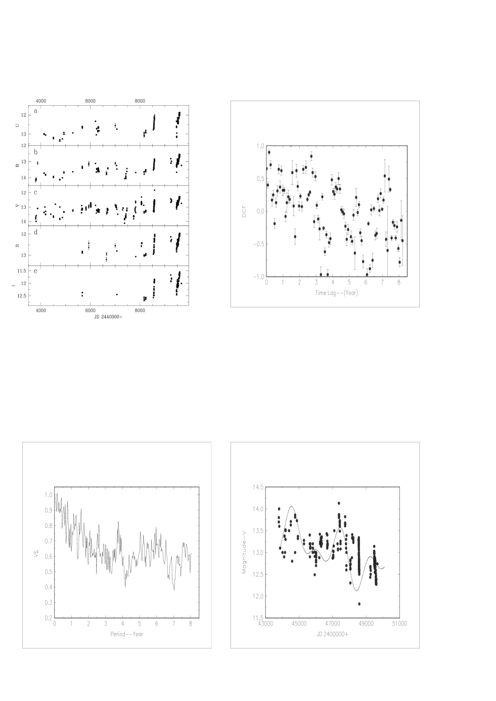
Figure 1: Fig1. Light curves of 2155-304; Fig 2. $V_{m}^{2}$ vs trial period of 2155-304; Fig 3. DCF analysis for 2155-304; Fig 4. The simulation light curve (solid curve) and the observation B light curve for 2155-304

The optical data used here are from the literature: Brindle et al. (1986); Carini & Miller (1992); Courvoisier et al. (1995); Griffiths et al. (1979); Hamuy & Maza (1987); Jannuzi et al. (1993); Mead et al. (1990); Miller & McAlister (1983); Pesce et al. (1997); Smith & Sitko (1991); Treves et al. (1989); Urry et al. (1993); Xie et al. (1996) and shown in Fig. 1a-e. From the data, the largest amplitude variabilities in UBVRI bands are found: $\Delta U=1^{m}.5(11^{m}.87-13^{m}.37)$; $\Delta B=1^{m}.65(12^{m}.55-14^{m}.20)$; $\Delta V=1^{m}.85(12^{m}.27-14^{m}.13)$; $\Delta R=1^{m}.25(11^{m}.96-13^{m}.21)$; $\Delta I=1^{m}.14(11^{m}.55-12^{m}.69)$. and color indexes are found: $(B-V)=0.30\pm 0.06$ (N=140 pairs); $(U-B)=-0.72\pm 0.08$ (N=105 pairs); $(B-R)=0.62\pm 0.07$ (N=90 pairs); $(V-R)=0.32\pm 0.04$ (N=98 pairs), the uncertainty is 1$\sigma$ dispersion.

2.2 Periodicity

The photometric observations of PKS 2155-304 indicate that it is variable on time scales ranging from days to years (Miller & McAlister 1983). Is there any periodicity in the light curve? To answer this question, the Jurkevich (1971) method is used to search for the periodicity in the V light curve since there are more observations in this band.

The Jurkevich method (Jurkevich 1971, also see Fan et al. 1998a) is based on the expected mean square deviation and it is less inclined to generate spurious periodicity than the Fourier analysis. It tests a run of trial periods around which the data are folded. All data are assigned to $m$ groups according to their phases around each trial period. The variance $V_{i}^{2}$ for each group and the sum $V_{m}^{2}$ of all groups are computed. If a trial period equals the true one, then $V_{m}^{2}$ reaches its minimum. So, a “good” period will give a much reduced variance relative to those given by other false trial periods and with almost constant values. To show the significance of the trial periodicity, we adopted the $F$-test (see Press et al. 1992).

When the Jerkevich method is used to V measurements, some results are obtained and shown in Fig. 2 ($m=10$), which shows several minima corresponding to trial periods of less than 4.0-year and two broad minima corresponding to averaged periods of (4.16 $\pm$ 0.2) and (7.0 $\pm$ 0.16) years respectively.

For the periods, which are smaller than 4.0-year, we found that the decrease of the $V_{m}^{2}$ is less than 3 times of the noise suggesting that it is difficult for one to take them as real signatures of periods, i.e., those periods should be discussed with more observations. For the two broad minima, the $F$-test is used to check their reality. The significance level is 93.8$\%$ for the 4.16-year period and 96.2$\%$ for the 7.0-year period.

3 Discussion

PKS 2155-304 was observed more than 100 years ago. Griffiths et al. (1979) constructed the annually averaged B light curve up to the 1950’s from Harvard photographic collection. But there are only a few observations during the period of 1950-1970. The periodicity obtained here (see Fig. 2) are based on the post-1977 data.

For comparison, we adopted the DCF (Discrete Correlation Function) method to the V measurements. The DCF method, described in detail by Edelson & Krolik (1988) (also see Fan et al. 1998b), is intended for analyses of the correlation of two data set. This method can indicate the correlation of two variable temporal series with a time lag, and can be applied to the periodicity analysis of a unique temporal data set. If there is a period, $P$, in the lightcurve, then the DCF should show clearly whether the data set is correlated with itself with time lags of $\tau$ = 0 and $\tau$ = $P$. It can be done as follows.

Firstly, we have calculated the set of unbinned correlation (UDCF) between data points in the two data streams $a$ and $b$, i.e.

$${UDCF_{ij}}={\frac{(a_{i}-\bar{a})\times(b_{j}-\bar{b})}{\sqrt{\sigma_{a}^{2}\times\sigma_{b}^{2}}}},$$ (1)

where $a_{i}$ and $b_{j}$ are points in the data sets, $\bar{a}$ and $\bar{b}$ are the average values of the data sets, and $\sigma_{a}$ and $\sigma_{b}$ are the corresponding standard deviations. Secondly, we have averaged the points sharing the same time lag by binning the $UDCF_{ij}$ in suitably sized time-bins in order to get the $DCF$ for each time lag $\tau$:

$${DCF(\tau)}=\frac{1}{M}\Sigma\;UDCF_{ij}(\tau),$$ (2)

where $M$ is the total number of pairs. The standard error for each bin is

$$\sigma(\tau)=\frac{1}{M-1}\{\Sigma\;[UDCF_{ij}-DCF(\tau)]^{2}\}^{0.5}.$$ (3)

The resulting DCF is shown in Fig. 3. Correlations are found with time lags of (4.20 $\pm$ 0.2) and ( 7.31 $\pm$ 0.16) years. In addition, there are signatures of correlation with time lags of less than 3.0 years. If we consider the two minima in both the right and left sides of the 7.0-year minimum, then we can say that the periods of 4.16 and 7.0-year found with Jerkevich method are consistent with the time lags of 4.2-year and 7.3-year found with the DCF method. These two periods are used to simulate the light curve (see the solid curve in Fig. 4).

It is clear that the solid curve does not fit the observations so well. One of the reasons is that there are probable more than two periods ($\sim$ 4.2 and $\sim$ 7.0 years) in the light curve as the results in Fig 2 and 3 indicate. Another reason is that the derived period is not so significant as Press (1978) mentioned. Press argued that periods of the order the third of the time span have a large probability to appear if longer-term variations exist. The data used here have a time coverage of about 16.0 years, i.e., about 3 times the derived periods. Therefore, these are only tentative and should be confirmed by independent work.”

From the data, the largest amplitude variations are found for UBVRI bands with I and R bands showing smaller amplitude variations. One of the reasons is from the fact that there are fewer observations for those two bands, another reason is perhaps from the effect of the host galaxy, which affects the two bands more seriously.

In this paper, the post-1970 UBVRI data are compiled for 2155-304 to discuss the spectral index properties and to search for the periodicity. Possible periods of 4.16 and 7.0 years are found.

Figure Captions

Fig. 1: a: The long-term U light curve of PKS 2155-304;
b: The long-term B light curve of PKS 2155-304;
c: The long-term V light curve of PKS 2155-304;
d: The long-term R light curve of PKS 2155-304;
e: The long-term I light curve of PKS 2155-304.

Fig. 2: Plot of $V_{m}^{2}$ vs. trial period, $P$, in years

Fig. 3: DCF for the V band data. It shows that the V light curve is self-correlated with time lags of 4.2 and 7.31 years. In addition, there are also correlation with time lags of less than 4.0 years.

Fig. 4: The observed V light curve (filled points) and the simulated V light curve (solid curve) with the periods of 4.16 and 7.0 considered.

References

- (1) Bertaud CH., Wlerick G., Vron P., et al. 1973, A&AS 11, 77
- (2) Bowyer S., Brodie J., Clarke J. T., Henry J.P. 1984, ApJ 278, L103
- (3) Brindle C., Hough J.H., Bailey J.A., et al. 1986, MNRAS 221, 739
- (4) Brown L.M.J., Robson E.I., Gear W.K., Smith M.G.: 1989, ApJ 340, 150
- (5) Chadwick P.M. et al. 1999, ApJ 513, 161
- (6) Carini M.T., Miller H.R., 1992, ApJ 385, 146
- (7) Charles P., Thorstensen J., Bowyer S., 1979, Nat. 281, 285
- (8) Courvoisier T.J.L., Blecha A., Bouchet P., et al., 1995, ApJ 438, 108
- (9) Edelson, R.A. & Krolik, J.H., 1988, ApJ, 333, 646
- (10) Fan J.H., Xie G.Z., Pecontal E., et al., 1998a, ApJ, 507, 173
- (11) Fan J.H., Adam G. Xie G.Z. et al., 1998b, A&AS, 136, 217
- (12) Fan J.H.: 1993, Ph.D. Thesis, Yunnan Astronomic Observatory, Chinese Academy of Sciences.
- (13) Fan J.H., Xie G.Z., Adam G. et al. 1999, ASP Conf. Ser. Vol. 159, Eds. L. Takalo & A. Sillanpaa, p99
- (14) Giommi P., Barr P., Garilli B., et al. 1991, ApJ 356, 432
- (15) Giommi P., Fiore F., Guainazzi M., et al. 1998, A&A 333, L5
- (16) Griffiths R. E., Briel U., Chaisson L., Tapia S., 1979, ApJ 234, 546
- (17) Hamuy M., Maza J., 1987, A&AS 68, 383
- (18) Jurkevich I. 1971, Ap&SS 13, 154
- (19) Jannuzi B.T., Smith P.S., Elston R., 1993, ApJS 85, 265
- (20) Mead A.R.G., Ballard K.R., Brand P.W.J.L., et al. 1990, A&AS 83, 183
- (21) Miller H.R., Carini M.T., 1991, in Variability of Active Galactic Nuclei, eds. H.R. Miller and P.J. Wiita (Cambridge: Cambridge Univ. Press), p256
- (22) Miller H.R., McAlister H.A., 1983, ApJ 272, 26
- (23) Paltani S., Courvoisier T.J.L., Blecha A., Bratschi P., 1997, A&A 327 539
- (24) Pesce J.E., Urry C.M., Maraschi L., et al. 1997, ApJ 486, 770
- (25) Pian E., Urry C.M., Pesce J.E. et al. 1996, in ’Blazar Continuum Variability’ eds. H.R. Miller, J.R. Webb, and J.C. Noble, ASP Conf. Series VoL. 110, 417
- (26) Press W.H. 1978 Comm. on Astrophys. 7, 103
- (27) Press W.H., Teukolsky S.A., Vetterling W.T., Flannery B.P. 1992, in Numerical Recipes in C, The Art of Scientific Computing (2nd Edition), Cambridge Uni. Press.
- (28) Smith P.S., Sitko M.L., 1991, ApJ 383, 580
- (29) Treves A., Morini M., Chiappetti L. et al. 1989, ApJ 341, 733
- (30) Urry C.M., Maraschi L., Edelson R. et al. 1993, ApJ 411, 614
- (31) Wade R.A., Szkody P., Crdova F., 1979, IAU Circ., No. 3279.
- (32) Zhang Y.H., Xie G.Z. 1996, A&AS 119, 199
- (33) Xie G.Z. et al. 1996, AJ, 111, 1065