A linear thermohaline oscillator driven by
stochastic atmospheric forcing
Stephen M. Griffies† and Eli Tziperman‡
† Princeton University
Atmospheric and Oceanic Sciences Program
Sayre Hall, Forrestal Campus
Princeton NJ 08544-0710. USA
email: smg@gfdl.gov
‡ Princeton University
Atmospheric and Oceanic Sciences Program
Sayre Hall, Forrestal Campus
Princeton NJ 08544-0710. USA
and
Department of Environmental Sciences
Weizmann Institute of Science
Rehovot, 76100. ISRAEL
email: citziper@weizmann.weizmann.ac.il
Revised submission to Journal of Climate
Los Alamos e-print ao-sci/9502002
Abstract
The interdecadal variability of a stochastically forced four-box model of the oceanic meridional thermohaline circulation (THC) is described and compared to the THC variability in the coupled ocean-atmosphere GCM of Delworth, Manabe, and Stouffer (1993). The box model is placed in a linearly stable thermally dominant mean state under mixed boundary conditions. A linear stability analysis of this state reveals one damped oscillatory THC mode in addition to purely damped modes. The variability of the model under a moderate amount of stochastic forcing, meant to emulate the random variability of the atmosphere affecting the coupled model’s interdecadal THC variability, is studied. A linear interpretation, in which the damped oscillatory mode is of primary importance, is sufficient for understanding the mechanism accounting for the stochastically forced variability. Direct comparison of the variability in the box model and coupled GCM reveals common qualitative aspects. Such a comparison supports, although does not verify, the hypothesis that the coupled model’s THC variability can be interpreted as the result of atmospheric weather exciting a linear damped oscillatory THC mode.
1 Introduction
The need to differentiate anthropogenic climate change from natural climate variability has generated intense research efforts directed at understanding and modeling climate variability. In particular, attention has focused on phenomena occurring on interdecadal or longer time scales. As it is believed that the ocean is a major climate component determining variability at these time scales, several ocean-only models as well as coupled ocean-atmosphere models of varying sophistication have been employed to study such variability and to identify its fundamental modes.
The meridional heat transport in the Atlantic basin is strongly dependent on the thermohaline circulation (THC). Hence, variability in the Atlantic’s THC is potentially connected with climate variability in and around the Atlantic. Much of the evidence for this connection, both from models and historical data, is discussed in the review by Weaver and Hughes (1992). Additional reviews are provided by Willebrand (1993) and Marotzke (1994).
Modeling efforts, from box-models (e.g., Stommel 1961) to fully coupled ocean-atmosphere GCMs (e.g. Delworth et al. 1993; hereafter D93), have indicated a suite of variability in the THC. The time scales of the model variability range from decadal and century (e.g., Weaver et al. 1991, 1993, 1994, Mikolajewicz et al. 1990, Weisse et al. 1994, Winton et al. 1993, Mysak et al. 1993, Moore and Reason 1993, Yin and Sarachik 1993, Greatbatch and Zhang 1994, Cai et al. 1994, and D93), associated with advective/convective mechanisms, to millennial (e.g., Marotzke 1989, 1990, Weaver and Sarachik 1991, and Weaver et al. 1993), associated with diffusive mechanisms. The amplitudes of the variability range from a small to rather large percentage of the mean circulation, associated with the interdecadal to century oscillations, to massive flushing events occurring on the millennial time scale. The variability studied in the ocean-only models has been predominantly associated with self-sustained oscillations involving non-linear mechanisms. The models of Mikolajewicz et al. 1990, Weisse et al. 1993, and Mysak et al. 1993 are exceptions in which the decadal and century variability is driven by stochastic salinity forcing in which a linear modal interpretation is available.
D93 have shown that the coupled ocean-atmosphere climate model developed at NOAA’s Geophysical Fluid Dynamics Laboratory exhibits small amplitude [ of the roughly Sv () mean meridional circulation] interdecadal ( years) thermohaline variability about a thermally dominant THC in the North Atlantic sector of their model. The basic mechanism identified for this variability is the advection of salt and heat into the northern “sinking region” creating periodically positive and negative density anomalies closely correlated to the circulation anomalies. The model variability seems to be associated with variability about a stable climate state rather than the larger fluctuations which may have occurred in the transition to or from an ice age (see Weaver and Hughes 1992 and references therein for a discussion of such transitions).
The small amplitude variability seen in D93 is consistent with, although a not proof of, a linear mechanism being responsible for the oscillatory behavior in the coupled model. For studying such an interpretation, the results of simplified models can provide useful insight. For example, Stommel (1961) found that a linear stability analysis of his thermohaline two–box model displayed a damped oscillatory response in part of its parameter range. As pointed out by Bryan and Hansen (1992) and Ruddick and Zhang (1994), the damped oscillatory response exists only in a saline dominant regime when the model is forced under mixed boundary conditions. Such a regime is not relevant for describing the present North Atlantic variability. However, the results of Tziperman et al. (1994, hereafter T94) indicated that when more degrees of freedom are considered, a damped oscillatory response within a thermally dominant regime can result from a box model. The damped oscillatory regime in T94 is near their four box model’s stability transition point; i.e., the point at which the model’s THC solution becomes unstable. They further suggested that their realistic-geometry primitive equation ocean GCM is near its stability transition point, possibly in the damped oscillatory regime found in their box model. Assuming that the variability found in D93 is due to a damped oscillatory mode, an external excitation of this mode is needed in order to sustain the variability. As noted in D93, such excitations may come from the random atmospheric weather. In this context, Bryan and Hansen (1992) considered the stochastic forcing of the thermally dominant state in the Stommel two-box model.
The purpose of this paper is to examine the hypothesis that the interdecadal variability observed in the coupled model analysis of D93 can be interpreted as the excitation of a damped oscillatory thermohaline mode by the stochastic effects of atmospheric variability. As a first step in testing this hypothesis, we investigate the variability of a highly simplified mixed boundary condition ocean-only four-box model of the oceanic meridional circulation forced by stochastic surface heating. A direct comparison of the box model variability to that of the coupled model shows a qualitative agreement between the mechanisms acting in the two models. Such agreement supports, although clearly cannot validate, the proposed hypothesis for the coupled model.
Some important aspects of the variability seen in the coupled model of D93 have been captured in the recent work of Greatbatch and Zhang (1993) using a three-dimensional planetary geostrophic ocean model forced with a zonally symmetric fixed heat flux and a zero salinity flux. This work was extended by Cai et al. (1994) to a primitive equation model with a zonally asymmetric fixed heat flux. Both of these studies identified variability of a gyre circulation in the North Atlantic similar to that identified by D93. However, the simulations of Greatbatch and Zhang and Cai et al. do not capture the temperature and salinity phase relations of D93 due to their use of a fixed heat flux. Although the two dimensional mixed boundary condition box model studied in this paper cannot capture the three-dimensional gyre-effect, we will argue that it does capture much of the zonally averaged variability acting in the coupled model; in particular, the phase relations between temperature/salinity and the THC are quite similar to that of D93. Both the temperature/salinity phase relations and the gyre effect are important parts of the variability seen in D93 and the full explanation of the coupled model’s variability probably includes both the mechanisms suggested here and in Greatbatch and Zhang and Cai et al. An additional important difference between the present work and that of Greatbatch and Zhang and Cai et al. is that the box model’s variability is linear and noise driven whereas that of Greatbatch and Zhang and Cai et al. is self-sustained and hence nonlinear in character. The different perspectives taken in this study and that of Greatbatch and Zhang and Cai et al., both of which seem to give reasonable agreement with various aspects of the coupled model’s variability, are perhaps part of a continuing dialogue necessary to successfully understand and simulate the ocean’s THC.
We begin in Section 2 with a detailed description of the box model and its linear stability properties while under mixed boundary conditions. The essential results from this section are summed up in Figs. 1 and 2 which show the box model configuration and its damped oscillatory response, respectively. It is the variability about such a stable, damped oscillatory steady state that is of interest in the following sections. Section 3 presents a linearized advective mechanism describing the box model’s damped oscillatory response to small perturbations about its thermally dominant steady state. In Section 4 we analyze the response of the box model subjected to stochastic heating on the surface boxes. The results from such variability are compared to the zonally averaged results from the coupled GCM of D93. We present further discussion in Section 5 and conclusions in Section 6.
2 The box model
Since the work of Stommel (1961), box models have proven to be a useful tool for studying the ocean’s THC because they allow for the examination of individual processes which might be important for the circulation’s stability and variability. Most often, and in this work too, the boxes have no zonal extent; i.e., the model has only two spatial dimensions which correspond to the vertical and meridional directions. Though highly idealized, the perspective taken here is that box models can provide a tool for testing hypotheses which can be directly compared against the results of more realistic models and observations.
2.1 Model equations
We consider a four-box model of a thermally dominated North Atlantic-like meridional circulation similar to those of Huang et al. (1992) and T94 (Fig. 1). Relatively warm salty boundary conditions are prescribed for the southern surface box and cold fresh boundary conditions are prescribed for the northern surface box. Due to the opposing effects of salinity and temperature on the density of sea water, salt contributes a southern sinking buoyancy torque and temperature creates a northern sinking torque. The model has no local convective mixing nor any explicit diffusion; hence, the temperature and salinity in each box are only affected by advection to and from neighboring boxes as well as by surface fluxes in the upper two boxes.
The steady state fields, about which variability is studied, are computed using restoring surface conditions for both the salinity and temperature. Thereafter, the implied salinity flux is fixed and the model is run with mixed boundary conditions (F. Bryan 1986). The temperature and salinity equations governing the box model in the absence of stochastic forcing are
| (1) | |||||
| (2) | |||||
| (3) | |||||
| (4) | |||||
| (5) | |||||
| (6) | |||||
| (7) | |||||
| (8) |
In these equations, the overdot indicates a time derivative, and are the box temperatures and salinities, are the restoring temperatures for the surface boxes, is the volume of the southern lower box (the largest box), is the circulation volume flow rate, and is the restoring time for the temperature. A salinity restoring condition is used for reaching a steady state, with the restoring time and the restoring salinities. Afterwards, the fixed flux is used for the mixed boundary conditions, with the barred quantities denoting the steady state values reached under restoring conditions. The steady state conditions, obtained by setting the time derivatives in equations (1)–(8) to zero, satisfy and for the thermally dominant flow considered here. The dimensionless numbers are geometric factors defined in Fig. 1. The differencing in equations (1)–(8) assumes a northern sinking thermal dominated circulation, which is that of interest in this study.
The circulation in the box model is driven solely by horizontal pressure gradients between the north and the south which, using the hydrostatic approximation, correspond to density gradients. A larger northern density creates a positive circulation. Therefore, the circulation is given by
| (9) |
where, assuming a linear equation of state, the densities in the boxes are with , and being the reference density, temperature, and salinity, respectively. The thermal and saline expansion coefficients and are taken as constants throughout the system which guarantees that the circulation (9) vanishes when the north–south temperature and salinity gradients vanish. The more realistic case in which and are different for the four boxes, as well as a nonlinear equation of state, should not qualitatively change the following results which consider only moderate variability.
The form of the advective circulation (9) is commonly chosen in Stommel-type box models, such as this model, which attempt to incorporate only advective processes. It should be noted that in a three dimensional circulation, east-west pressure gradients, through geostrophy, typically are associated with meridional flow rather than north-south gradients. In the formulation of their zonally averaged ocean model, Wright and Stocker (1991) provide some heuristic motivation for using such a parametrization starting from three dimensional equations of motion. Additionally, the study by Hughes and Weaver (1994) provides evidence that the meridional circulation in their three dimensional model is directly proportional to the north-south steric height difference, further motivating the parametrization (9). Finally, the results exhibited in the coupled model of D93 to be described below, and the qualitative agreement of the box model with these results, suggest this choice for the current study.
2.2 Box parameters
The parameters used for the box model experiments are as follows. In the linear equation of state, the parameters , and kg/m3 represent values for and psu. The surface restoring temperatures and salinities , , , and are chosen along with the temperature restoring time days to yield reasonable steady state conditions under restoring conditions. The salinity restoring coefficient ) is chosen to give a box model response emulating that of the coupled model of D93, as further discussed in Section 4. The geometry of the box model roughly reflects the region of the Atlantic from the equator northward. The sinking in the coupled model is localized in a small region within this northern latitude band; hence, the latitudinal width ratio (see Fig. 1) is chosen. The depth ratio is and the volume of the largest box (southern deep box) is . With this thickness for the upper boxes (300 meters), the temperature restoring time corresponds to that commonly taken in ocean-only GCM studies (e.g., Tziperman and Bryan, 1993 which use 30 days for a 50 meter upper layer). Finally, the circulation parameter Sv results in a mean circulation on the order of that seen in D93.
The above parameters, though chosen to roughly reflect the Atlantic basin in the coupled model of D93, are not meant to be quantitatively precise. Rather, it is the purpose of the box model study to illustrate a particular mode of variability emulating that seen in the coupled model. Precise quantitative correspondence is not pursued. Along these lines, it should be noted that we have found these oscillations to occur over quite a broad range of box model parameters.
2.3 Linear stability
In order to investigate the model’s stability to small perturbations, we consider the governing equations (1)–(8) under the mixed boundary conditions and linearized about the steady state obtained with restoring boundary conditions;
| (10) | |||||
| (11) | |||||
| (12) | |||||
| (13) | |||||
| (14) | |||||
| (15) | |||||
| (16) | |||||
| (17) |
where , and are the temperature, salinity, and circulation anomalies, respectively. The set of linear equations (10)–(17) can be written in the matrix vector form , where the vector has eight components consisting of the four temperature and four salinity anomalies. is an matrix dependent on the model parameters and the underlying steady state reached under restoring conditions (Marotzke 1990, T94).
A stability analysis of the linear equations (10)–(17) was carried out in T94. As found there, should the salinity torque become large enough to overcome the effects of the temperature torque [explicitly, if with in the example discussed in T94], the thermally dominant mean circulation will be unstable to small perturbations, and such a perturbation would result in the system making a transition to a stable saline dominant mean state of opposite circulation direction. Increasing the salinity forcing in this model (e.g., using a smaller salinity restoring time ) when initializing under restoring conditions results in a larger mean salinity gradient and hence a larger salinity torque. A continuum of linear response is thus found as the salinity forcing is increased. Namely, the stability behavior to small perturbations changes from that of a purely exponential decay of the perturbation for small salinity forcing, to oscillatory decaying response, to oscillatory growing behavior, and finally, for a strong enough salinity forcing, to small perturbations growing exponentially without any oscillations. These stability results are further discussed in T94 where a detailed stability analysis for the damped oscillatory regime is given.
The regime of interest in the following is that linearly stable thermally dominant state which responds in a damped oscillatory manner to small perturbations. More precisely, the linearized system in the following will contain a single damped oscillatory eigenmode (and its complex conjugate) with the remaining eigenmodes purely damped. The damped oscillatory mode forms the basis for the model’s variability studied in this work.
3 Linear thermohaline oscillations
We now examine the response of the box model, described by the nonlinear conservation equations (1)–(8), to an instantaneous heat perturbation when the model is placed in a stable damped oscillatory regime under mixed boundary conditions. Note that a forward Euler time stepping scheme is employed for the numerical realizations of the box model equations (1)–(8) with 365 time steps per model year. There are no noticeable differences between these results and those obtained when we used a leapfrog scheme with intermittent Euler forward stepping to suppress the computational mode. As the numerical results are consistent with the eigenvalue analysis discussed in the previous section, we are confident that the variability reported here is that of the underlying physical processes acting in the box model and are not adversely affected by numerical artifacts such as truncation and numerical dissipation.
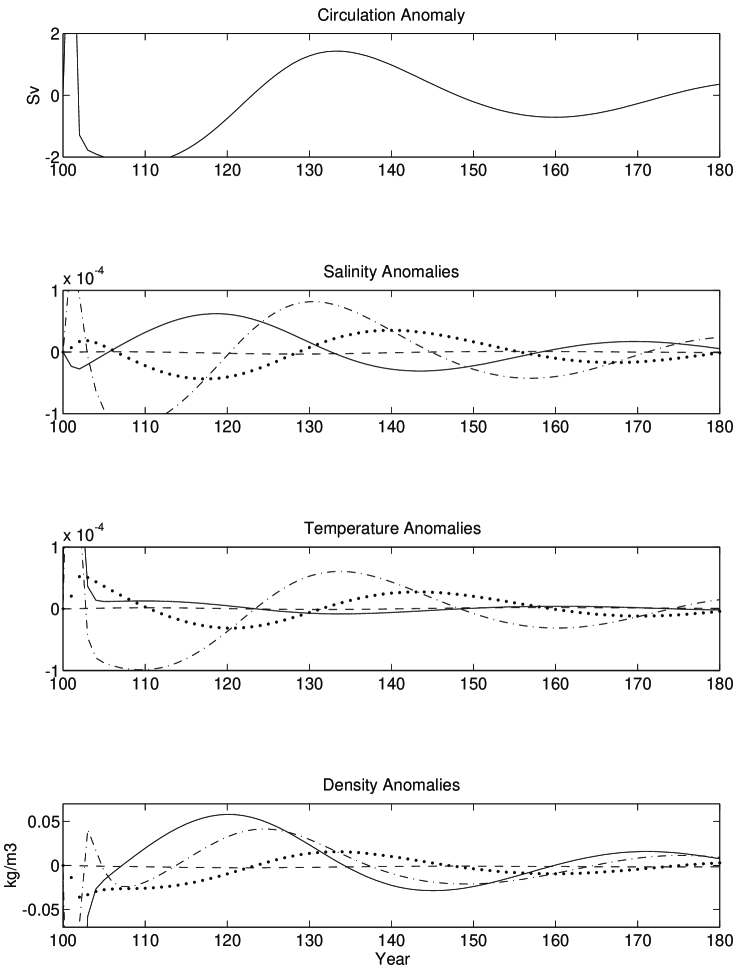
Fig. 2 shows the circulation, salinity, temperature, and density anomalies for the mixed boundary condition model as it responds to a relatively large perturbation consisting of a cold surface anomaly in the north (box ) and a warm surface anomaly in the south (box ). The steady state conditions are , and Sv. The temperature and salinity anomalies shown in Fig. 2 are multiplied by their respective expansion coefficients and allowing for a direct comparison of the relative contributions each field makes to the density anomalies and hence to the circulation anomaly.
The result of the perturbation is a positive circulation anomaly. The phases and relative amplitudes shown in Fig. 2 are quite similar to those of the damped oscillatory eigenmode (not shown) of the linearized system, whose period and decay time are and years, respectively. Therefore, although the initial perturbation projects onto various eigenmodes, the system’s response is dominated by the damped oscillatory eigenmode of the linearized system after a relatively short adjustment time.
The relative phases of the oscillation between the different boxes can be understood as time delays for the advection of the anomalous water through the boxes. The amount of delay for the advection is directly related to the size of the box. The relative amplitude of the oscillation within a box is also related to the sizes of the boxes, with the largest box (box 3) exhibiting the smallest amplitude. Additionally, the surface temperature anomalies, as they are damped by the atmospheric restoring, are reduced in amplitude relative to the surface salinity anomalies which are not damped under the fixed fluxes. The temperature anomalies are hence slightly subdominant to the salinity anomalies in their contribution to the anomalous circulation. Nevertheless, temperature effects play an important and non-negligible part in the physical mechanism responsible for the model’s oscillations, as explained in the following.
The temperature and salinity perturbations within each box determine the circulation anomaly passing through all boxes. The circulation anomaly in turn creates a feedback to the temperature and salinity in the individual boxes. Note that the results reported throughout this paper are generated by the full nonlinear conservation equations (13)–(17). However, since the model is exhibiting a very linear response, it is useful for understanding the physical mechanism of this damped oscillation to follow a cycle with reference made to the linear equations (13)–(17).
We begin with the growing phase of a positive circulation anomaly (e.g., year 125–130 in Fig. 2), where the positive circulation anomaly advects the mean high salinity and mean high temperature water from the southern surface box (box 1) to the northern surface box (box 2) which drives up the salt and temperature anomalies in the north [see in particular the first terms of the right hand side of eqns. (11) and (15)]. A comparison of Figs. 2A and 2B indicates that the growth in dimensionless salinity anomaly dominates the dimensionless temperature anomaly during this portion of the oscillation because of the effects of the atmospheric restoring term () on the warm water advected from box 1. This process drives up the northern density which amplifies the growing circulation anomaly and thus represents a positive feedback. Note that during this buildup of salty water in the north, a fresh cold anomaly develops in the southern upper box 1. So far the discussion parallels the thermohaline instability mechanism under mixed boundary conditions described by Walin (1985) and Marotzke et al. (1988), in which the temperature variations are neglected.
The positive feedback of added salinity in the north eventually yields, within a few years, to a negative feedback due to the warm water also advected northward which reduces the growth of the northern density and therefore the circulation anomaly as well. The negative feedback from temperature eventually causes the circulation anomaly and the northern density to reach a maximum. The peaking of the northern density causes the circulation anomaly to likewise reach a maximum and thereafter begin the decreasing portion of its oscillation. The extremum reached by the density in a box corresponds to the interchange in dominance between the competing terms in the linearized equations (10)–(17). In particular, when the circulation anomaly has weakened sufficiently due to the temperature feedback, the advection of the anomalous temperature and salinity gradients by the mean circulation [i.e., and ] dominates the advection of the mean gradients by the circulation anomaly [ i.e., and ]; cf. equs. (11) and (15). This interchange in dominance has a stabilizing effect and causes both the temperature and salinity of box 2 to continue decreasing. The atmospheric restoring term also cools the warm water pool formed in box 2, again reducing the temperature perturbation towards zero.
Once the circulation anomaly approaches the zero crossing point, the perturbation temperature and salinity in the northern boxes are also approaching the zero crossing point. Because of the phase lag between the north and south, there is still a significant fresh cold anomaly in the southern box 1 which is now advected by the mean flow to the north. This advection forces the zero crossing of the temperature and salinity perturbations in the north and creates a negative density anomaly. This density anomaly induces a negative circulation anomaly; i.e., it weakens the total circulation. The same cycle described above now repeats but with the opposite temperature, salinity, density and circulation anomalies. In this opposite portion of the oscillation, the negative circulation anomaly, which is initially strengthened in absolute value by the positive feedback created by the negative salinity anomaly in the north, will reach an extremum when the negative feedback due to the negative temperature anomaly in the north kicks in. The circulation anomaly thereafter increases towards zero again, thus completing one full cycle.
It should be re-emphasized that although temperature anomalies are slightly subdominant to salinity anomalies in their contribution to the box model’s circulation anomaly, their effects are non-negligible in the physical mechanism presented here. For example, in the absence of the negative feedback from temperature, a thermally dominant steady state is unstable to perturbations. This behaviour, which is clear from the mechanism previously described, can be verified mathematically by considering the response of the model when the temperature feedback is suppressed. In particular, a linear stability analysis for a fixed temperature perturbation (all temperatures are held to their steady state values) yields exponentially growing non-oscillatory eigenmodes signaling an instability. Conversely, perturbations to the model in which the salinity feedback is suppressed are exponentially damped and non-oscillatory due to the absence of a positive feedback in the system.
Therefore, the linear mechanism for the oscillations relies on three main factors: a positive feedback from salinity that creates a growth in the absolute value of the salinity, temperature and circulation anomalies; a negative feedback from temperature, following a few years after the positive feedback from salinity, that dampens the growth caused by the salinity feedback allowing the anomalies to reach a local extremum; and a time delay between the temperature and salinity in the southern and northern boxes that allows for the zero crossing of the oscillating perturbations. Finally, the overall damping of the oscillations seen in Fig. 2 reflects the dominance of the temperature feedbacks for the perturbations about this particular steady state.
An important element of the oscillation mechanism described above, as well as that discussed by D93 for the coupled model, is the phase lag between the temperature and salinity within a particular region of the respective models. This lag in the box model is a direct result of the different boundary conditions for the temperature and salinity. When both temperature and salinity have the same boundary conditions, whether a fixed and fixed heat flux or restoring conditions with the same restoring times, the temperature and salinity equations can be reduced to a single density equation when a linear equation of state is used. Model variability will therefore have either a zero or 180 degree phase difference between the anomalous temperature and salinity fields thus making the variability density driven rather than thermohaline (i.e., temperature and salinity) driven. Breaking the symmetry between temperature and salinity forcing, as through mixed boundary conditions, allows the two fields to no longer have such a constrained phase relationship thus enabling the existence of the linear thermohaline oscillations described here.
It is useful to compare the oscillations described here to the Howard-Malkus loop oscillations described by Welander (1986) and more recently by Winton and Sarachik (1993). Since both oscillators are advective in nature, their period is related to the time for the advection of anomalous fields through the respective systems. In the loop systems, self-sustained nonlinear oscillations are possible due to the existence of unstable equilibria which result in a limit cycle mechanism. The oscillations described here result from linear perturbations about a stable equilibrium and are hence exponentially decaying and not self-sustaining.
4 Stochastically forced thermohaline oscillations
In this section, we consider the response of the box model to stochastic forcing on the surface boxes under mixed boundary conditions. This forcing is meant to approximate the effects of synoptic scale atmospheric variability on the air-sea fluxes present in the coupled model of D93. The numerical realization of the stochastic forcing follows that described by Kloeden and Platen (1992) (for a mathematical discussion) and Penland (1989) (for meteorological examples). The response of the fully nonlinear box model to a single perturbation in Section 3 was understood as being predominantly the response of the model’s damped oscillatory eigenmode from the linearized system. This linear interpretation will also hold in the following for the model when driven with a moderate amount of stochastic forcing.
4.1 The stochastic forcing
To motivate the form of the stochastic forcing acting on the surface boxes, it is useful to consider the results of D93 for the regression of the zonally averaged anomalous heat and salinity budgets in the northern sinking region of their model against the anomalous THC index (Figs. 14 and 15 of D93, respectively). The regression coefficient at all lag times for the anomalous surface () flux is very small relative to that for the salinity transported by the meridional oceanic circulation from the south. While this does not imply a small () flux over the synoptic time scale of the coupled model’s atmospheric variability, it does indicate that the variability in the surface salinity forcing over the model’s sinking region has a negligible contribution to the interdecadal THC variability. We therefore choose to set the anomalous () forcing to zero in the following box model study.
The regression coefficients for the coupled model’s anomalous surface heat flux are of similar magnitude to those from the meridional heat transported by the oceanic circulation from the south. Therefore, we expect the variability in the surface heating to be important for the THC variability and we therefore use an anomalous stochastic heat forcing in the following. Furthermore, since the interdecadal time scale of interest here is so much longer than the typical synoptic atmospheric weather phenomena, the stochastic heating will be modeled as an additive white noise heating. Experiments with nonzero auto-correlation (not shown) give qualitatively similar results to those reported here for the white noise heating.
To include the stochastic heating, the surface box temperature equations (1) and (2) are modified to the following form with additive white noise forcing
| (18) | |||||
| (19) |
In these expressions, is an adjustable noise level scaling and are independent Gaussian distributed, unit variance white noise processes. A value of is used in the following experiments, which indicates a white noise forcing with standard deviation the magnitude of the steady state heat flux. The white noise forcing is added every time step (365 time steps per year) during the integration. The remaining box model parameters are those given in Section 3.
Both the box model and the coupled GCM contain rapidly de-correlating processes that are not of direct interest in the present study. Therefore, to focus on the interdecadal response of the models, a year low pass filter is applied to the yearly averaged signals generated from the box model. The coupled model contains a trend which is roughly linear over the years of integration considered here. As described in D93, this trend is removed and then a -year low pass filter is applied to the yearly averaged fields. The subsequent analyses presented here consider only the low pass anomalous fields generated from both models.
4.2 Box model–coupled GCM comparison
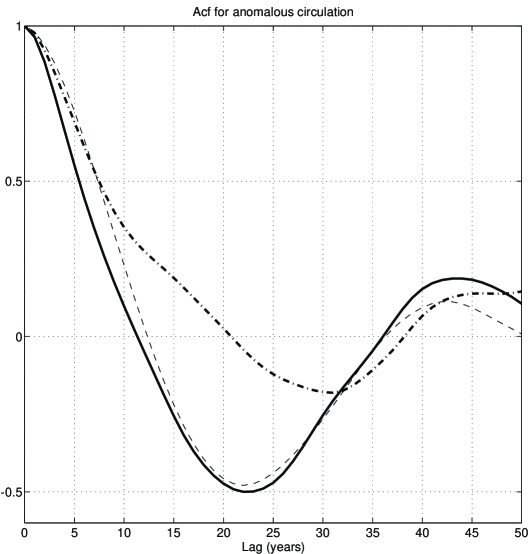
In this and the subsequent section, we compare part of the analysis of a year simulation from the coupled model of D93 to a year simulation from the box model. The statistics presented below for the box model were validated by using significantly longer time series. Since the ocean portion of the coupled model did not make a transition to a new equilibrium during the millennium integrated, the ocean will be considered to be in a stable climate regime. Likewise, the box model will be put in a thermally dominant regime such as that considered in Section 3. The auto-correlation function of both the THC index, defined as the maximum yearly averaged transport within the coupled model’s North Atlantic region, and the box model’s circulation anomaly are used as a diagnostic for determining the precise regime of the box model roughly corresponding to the coupled model’s behaviour.
Fig. 3 shows the auto-correlation function for the THC index from the coupled model (solid line) as well as for the circulation anomaly from the stochastically forced box model. For the box model, we present the circulation’s auto-correlation function resulting from two different salinity forcings. The dot-dashed line is the auto-correlation for the model placed in a highly damped oscillatory regime. For this experiment, the salinity restoring time, used to calculate the steady state before switching to mixed boundary conditions and the subsequent stochastic forcing, is set to days. The resulting salinity forcing for the mixed boundary condition integration is relatively weak which results in a highly damped oscillatory response. The resulting steady state circulation Sv. The damped oscillatory eigenmode of the system linearized about this steady state has period and e-folding time of and years, respectively. The dashed line in Fig. 3, which closely follows the auto-correlation function from the coupled model, is the result of using the salinity restoring coefficient of days which was considered in Sections 2.2 and 3. Motivated by the close correspondence between the auto-correlation functions of the coupled model and that of the box model spun up with days, we further study the variability of the mixed boundary condition box model spun up with this salinity forcing and compare to the coupled model results.
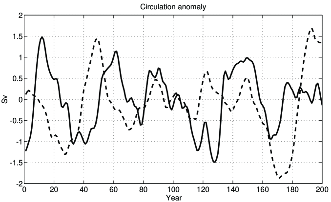
The time series for the annually averaged anomalous meridional circulation in the box model driven by stochastic forcing is shown in Fig. 4. The power spectra for this time series (not shown) has power broadly centered at a period of years, reflecting the contribution of the damped oscillatory eigenmode for the variability in the stochastically forced system. The corresponding time series for the thermohaline index from D93 is also shown in Fig. 4. The power spectrum for this time series, shown in Fig. 5 of D93, has power broadly centered around – years.
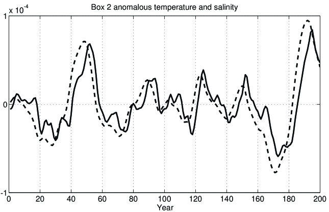
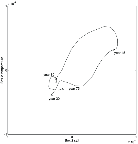
The time series for the temperature and salinity in the northern top box (box ) in the box model are shown in Fig. 5A. The response of the remaining larger boxes (not shown) are smoother and of smaller amplitude than the surface boxes reflecting an integrating property of the box model in its response to surface stochastic forcing. The phase relation (salt leads temperature), also present in the oscillating eigenmode shown in Fig. 2, reflects the dominance of this mode in determining the response of the stochastically forced system. The phase relations are further illustrated in the ( plane shown in Fig.5B. As salt leads temperature, the roughly circular trajectory traced out in this diagram is in the counterclockwise direction.
4.3 Linear regression analysis
In order to explore the physical mechanism of the interdecadal variability using time series from the coupled model, D93 computed the linear regression coefficients between the time series of selected model fields in the “sinking region” (N to N) of the North Atlantic portion of their model against the time series for the meridional circulation anomaly in the same region. This analysis provides information concerning the phase relations between the circulation anomaly and the regressed field; information which may be obscured in the individual noisy time series. For comparing these results with those of the box model, we employ the same regression analysis here.
The linear regressions involve the least squares fit of a linear relation between a selected anomalous field (e.g., salinity, heat flux, etc.) and the circulation anomaly over lagged portions of their respective time series of length years); i.e., we compute a regression coefficient at each lag by minimizing the quantity
| (20) |
For lags , the sum runs from to and the arguments and are used. The regression coefficient will be presented for lags years. Note that negative lags represent times prior to the maxima of the THC and positive lags are times subsequent to the maxima.
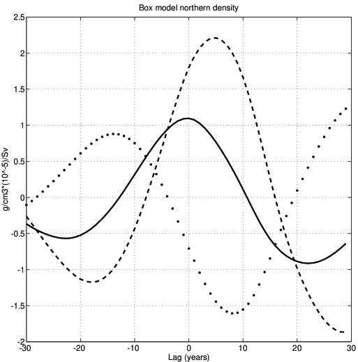
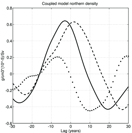
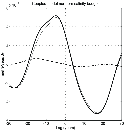
Fig. 6A shows the regression coefficient of the box model density anomaly spatially averaged over the northern boxes, , and its temperature and salinity contributions. The density peaks at lag zero indicating that the northern density is in phase with the circulation, a fact consistent with the damped oscillatory eigenmode dominating the oscillations as can be deduced from the time series in Fig. 2. Fig. 6B shows the corresponding regression from the coupled model for its sinking region.
Comparison of the two regressions reveals some of the similarities and differences between the two models’ THC variability. Notably, the box model salt and temperature contributions to density have similar relative phases as in the coupled model. Additionally, both models indicate that salinity is the dominant contributor to the density anomaly, and hence to the overall circulation anomaly. As mentioned previously, it is the damping of surface temperature anomalies which reduces their response relative to salinity anomalies in the box model. The magnitudes of the regression coefficients are larger in the box model than in the coupled model. This quantitative difference is, however, not unexpected considering the idealized nature of the box model. The phase difference between salt and temperature contributions to the density as seen in the box model is larger than that of the coupled model.
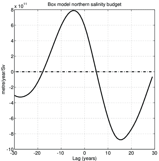
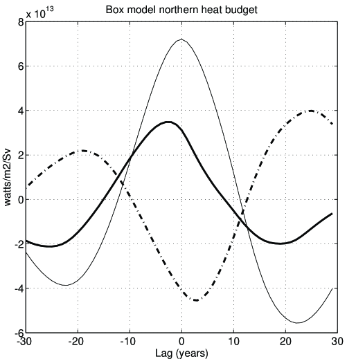
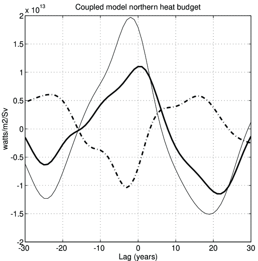
Fig. 7A shows the regression coefficients for the anomalous salinity budget transported into the northern box through the surface as well as that transported by the ocean from the south. Fig. 7B shows the corresponding regression for the coupled model. Note that in D93, a southward oceanic meridional transport into the sinking region from the extreme northern sector of the model was also included in their regression analysis. This transport contributes a negligible amount to the regression coefficients and is therefore not reproduced here. The box model budget of Fig. 7A is implied from the salinity transports divided by a reference salinity of psu. Recall that the anomalous surface salinity flux in the box model is set to zero. Figs. 8A,B present the corresponding regression coefficients for the heat budget in the two models. The sign conventions are such that a positive regression coefficient implies a positive anomalous transport into the northern portion of the model ocean (i.e., positive salinity and positive heat) for a positive anomalous circulation.
In the coupled model, an anomalous gyre transport plays an important role in advecting a positive salinity anomaly into the north previous to the THC maximum. Comparison of Fig. 7A with the regression for the coupled model in Fig. 7B indicates that without the gyre, the box model also brings a positive salinity anomaly into the north prior to the maximum of the THC, hence emulating the transport exhibited in the coupled model. The similarity of the variability in the two models might suggest that the gyre transport may be essential for establishing the detailed structure of the variability, yet perhaps the existence of the oscillation could be explained without the gyre effect. We note that Greatbatch and Zhang (1993) found a gyre effect similar to D93 induced by meridional oscillations based on a thermal only mechanism (i.e., the salinity was fixed in this model so that its oscillation mechanism is not thermohaline but rather single component).
Both the box and coupled models exhibit the same respective order of magnitude for the contributions of the surface and meridional heat transports into the northern region. This result is an important element of the box model oscillation and is associated with the restoring conditions placed on the surface temperature. Recall that a different perspective has been taken in the study of Greatbatch and Zhang (1994) and Cai et al. (1994) who study the THC oscillations in a model forced with a fixed surface heat flux; i.e., a zero anomalous surface heating. Their justification for considering this forcing was based on the dominance of the anomalous meridional heat transport over the anomalous surface heat transport in the coupled model THC variability, as revealed by the regression plot in Fig. 8B. We chose the conventional mixed boundary conditions formulation for the box model study to emulate the non-trivial phase relations between salinity and temperature and the THC seen in the coupled model. Such relations are not found in models forced with fixed heat and salinity fluxes. Additionally, both the box and coupled models have their surface and meridional heat transport components roughly out of phase. This similarity indicates that both models respond to the increasing circulation by bringing more warm water northward, with the peak happening near the peak of the THC. Note that the qualitative agreement between the models’ salinity regressions shown in Figs. 7A,B motivated the neglect of an anomalous surface salinity flux in the box model study.
5 Discussion
The mechanism operating in the box model oscillations is advective. Consequently, the period of the oscillations was found to be sensitive to the volume of the “sinking region” of the box model (boxes 2 and 4). If a similar dependence exists in the coupled model, this result may suggest that a more realistic higher resolution ocean model than that of D93, in which the extent of the sinking region may change, could result in a different time scale for the variability than that found in D93.
It is useful to contrast the roles played by temperature and salinity during the oscillations with their roles in establishing the underlying mean circulation. For the mean circulation, cold temperatures in the north and warm temperatures in the south act to set up a circulation with sinking in the north. Conversely, the buoyancy torque contributed by salinity acts to brake the mean thermally dominant circulation. If strong enough, the salinity torque causes the system to make a transition to the saline dominant circulation. For the thermohaline oscillations about a stable thermally dominant circulation, temperature effects act to move the anomalies back towards zero and thus acts as a negative feedback to the oscillations. Salinity effects, on the other hand, act to increase the magnitude of the oscillations and thus act as positive feedbacks.
A comment regarding the suitability of the mixed boundary conditions ocean-only models for simulating the thermohaline circulation is appropriate here. Willebrand (1993) and Marotzke (1994) identify certain feedbacks between the oceanic and atmospheric heat and moisture budgets important for establishing the large-scale stability of the underlying mean oceanic state. Leaving out some of these feedbacks, as done when conventional mixed boundary conditions are employed in ocean-only models, may lead to an unrealistic stability analysis. Indeed, mixed boundary condition ocean-only GCMs are perhaps more unstable than models more completely incorporating these feedbacks (e.g., Zhang et al. 1993, T94, and Rahmstorf and Willebrand 1994). In the present study, we have therefore placed the mixed boundary condition box model in a stable regime. Note that the stability of the box model solution, reflected in the decay time of the damped oscillations, is sensitive to boundary conditions through both the temperature restoring time and salinity forcing amplitude determined by . This result has been seen in other studies of the THC (e.g., Zhang et al. 1993, Power and Kleeman 1994, Marotzke 1994, Weaver et al. 1991, and T94). In order to study the mechanism suggested here in an ocean-only GCM, the GCM would need to be also placed in a stable regime under mixed boundary conditions by modifying both the salinity forcing (Weaver et al. 1991, and T94) and temperature restoring time (Zhang et al. 1993 and Power and Kleeman 1994). Furthermore, the GCM should be placed near enough to the stability transition point (T94) to allow for the non-trivial contributions of both temperature and salinity as described here.
6 Conclusions
We have considered the interdecadal variability in an ocean-only four-box model of the meridional thermohaline circulation (THC) and compared these oscillations with those found in the coupled ocean-atmosphere model of D93. The box model contains only advective processes which in turn render its governing equations (1)–(8) nonlinear. However, the small amplitude ( the mean circulation) response of the box model, of interest in the present study, can be given a straightforward linear interpretation.
The box model was placed in a stable thermally dominant mean circulation steady state under mixed boundary conditions. The model linearized about this state contains a single exponentially damped oscillatory eigenmode; all other modes are decaying and non-oscillatory and of little importance for understanding the model’s low frequency, small amplitude oscillatory variability. The presence of a moderate amount of stochastic surface heating (standard deviation the steady state heat flux), emulating the random forcing due to atmospheric weather, drives an effectively linear box model variability dominated by the damped oscillatory mode. Three main factors proved essential for the box model thermohaline oscillations: a positive feedback from salinity produces the initial growth in the absolute value of the anomalous fields and circulation; a negative feedback from temperature, following the effects of salinity, is responsible for the variability reaching a local extremum and thereafter approaching a zero anomaly; and a time delay between the temperature and salinity in the southern and northern boxes allowing for the zero crossing of the oscillating anomalies. For the stable state considered in this paper, the temperature feedbacks dominate the salinity feedbacks over the course of an oscillation which therefore yield a damped oscillatory response.
Although the box model results reported here are taken from the nonlinear model represented by the governing equations (1)–(8), the model’s variability is of a linear noise driven character arising from the random excitation of a single damped oscillatory thermohaline eigenmode. This result should be contrasted to those ocean-only models investigating the internal variability of the ocean which tend to focus on regimes controlled by self-sustaining nonlinear mechanisms which do not require external forcing (e.g., Weaver et al. 1991, 1993, 1994, Winton et al. 1993, Moore and Reason 1993, Marotzke 1989, 1990, Yin and Sarachik 1993, Yin 1993, and Greatbatch and Zhang 1993, Cai et al. 1994).
The qualitative agreement of the interdecadal THC variability seen in the stochastically driven box model and the coupled ocean-atmosphere GCM supports the view that the coupled model’s variability can be interpreted in a linear manner analogous to that of the box model. More precisely, the comparison supports the hypothesis that the fundamental meridional mode of low frequency variability in the coupled model’s THC is that of a damped oscillatory thermohaline mode driven by atmospheric weather. It is this stable linear hypothesis for the coupled model’s variability, and its support from the box model study, that is the main result of the present study. Nevertheless, at the conclusion of this study, the hypothesis for the coupled model remains speculative. Further work is clearly necessary to examine the linear noise-driven interpretation of both the coupled GCM and the actual climate system.
Acknowledgments. It is a pleasure to thank Kirk Bryan and Tom Delworth for their valuable insights and comments given throughout this project. Furthermore, additional thanks go to Tom Delworth for generously providing us with the results of D93. Thanks go to Isaac Held and Cecile Penland for useful comments and suggestions. Richard Greatbatch provided a very thorough and useful review. Funding for SMG is provided by a fellowship from the NOAA Postdoctoral Program in Climate and Global Change and NOAA’s Geophysical Fluid Dynamics Laboratory. We thank GFDL for its hospitality and support.
7 Bibliography
-
Bryan, F., 1986: High-latitude salinity effects and interhemispheric thermohaline circulations. Nature, 323, 301–304.
-
Bryan, K. and F.C. Hansen, 1992: A stochastic model of North Atlantic climate variability on a decade to century time-scale. Proceedings of the Workshop on Decade-to-Century Time Scales of Climate Variability, National Research Council, Board on Atmospheric Sciences and Climate, National Academy of Sciences, Irvine,CA, September, 1992.
-
Cai, W., R.J. Greatbatch, and S. Zhang, Interdecadal variability in an ocean model driven by a small zonal redistribution of the surface buoyancy flux. Journal of Physical Oceanography in press.
-
Delworth, T., S. Manabe, R.J. Stouffer, 1993: Interdecadal variations of the thermohaline circulation in a coupled ocean-atmosphere model. Journal of Climate, 12, 1993–2011.
-
Greatbatch, R.J. and S. Zhang, 1994: An interdecadal oscillation in an idealized ocean basin forced by constant heat flux. J. of Climate in press.
-
Huang, R.X., J.R. Luyten, and H.M. Stommel, 1992: Multiple equilibria states in combined thermal and saline circulation. J. Phys. Oceanogr., 22, 231–246.
-
Hughes, T.M.C. and A.J. Weaver, 1994: Multiple equilibria of an asymmetric two-basin ocean model. Journal of Physical Oceanography, 24, 619–637.
-
Kloeden, and Platen, 1992: Numerical Solution of Stochastic Differential Equations, Springer-Verlag.
-
Marotzke, J., 1989: Instabilities and multiple steady states of the thermohaline circulation. Oceanic Circulation Models: Combining Data and Dynamics, D.L.T. Anderson and J. Willebrand, Eds., NATO ASI series, Kluwer, 501–511.
-
Marotzke, J., 1990: Instabilities and multiple equilibria of the thermohaline circulation. Ph.D. thesis. Berlin Instit Meereskunde Kiel, 126 pp.
-
Marotzke, J., P. Welander, and J. Willebrand, 1988: Instabilities and multiple steady states in a meridional-plane model of the thermohaline circulation. Tellus, 40A, 162–172.
-
Marotzke, J., 1994: Ocean models in climate problems. Ocean Processes in Climate Dynamics: Global and Mediterranean Examples, P. Malanotte-Rizzoli and A.R. Robinson, eds., Kluwer Academic Publishers.
-
Mikolajewicz, U., and E. Maier-Reimer, 1990: Internal secular variability in an ocean general circulation model. Climate Dynamics, 4, 145–156.
-
Moore, A.M. and C.J.C. Reason, 1993: The response of a global general circulation model to climatological surface boundary conditions for temperature and salinity. J. Phys. Oceanogr., 23, 300–328.
-
Mysak, L.A., T.F. Stocker, and F. Huang, 1993: Century-scale variability in a randomly forced, two-dimensional thermohaline ocean circulation model. Climate Dynamics, 8, 103–116.
-
Penland, C., 1989: Random forcing and forecasting using principal oscillation pattern analysis. Monthly Weather Review, 117, 2165–2185.
-
Power, S.B. and R. Kleeman, 1993: Multiple equilibria in a global ocean general circulation model. J. Phys. Oceanogr., 23, 1670–1681.
-
Rahmstorf, S. and J. Willebrand, 1994: The role of temperature feedback in stabilising the thermohaline circulation. Journal of Physical Oceanography in press.
-
Ruddick, B. and L. Zhang, 1994: On the qualitative behaviour an non-oscillation of Stommel’s thermohaline box model. Journal of Climate submitted.
-
Stommel, H., 1961: Thermohaline convection with two stable regimes of flow. Tellus, 13, 224–230.
-
Tziperman, E. and K. Bryan, 1993: Estimating global air-sea fluxes from surface properties and from climatological flux data using an oceanic general circulation model. Journal of Geophysical Research, 98, 22629–22644.
-
Tziperman, E., R. Toggweiler, Y. Feliks, and K. Bryan, 1994: Instability of the thermohaline circulation with respect to mixed boundary conditions: Is it really a problem for realistic models? J. Phys. Oceanogr., 24, 217–232.
-
Walin, G., 1985: The thermohaline circulation and the control of ice ages. Paleogeography, Paleoclimatology, and Paleoecology, 50, 323–332.
-
Weaver, A.J. and E.S. Sarachik 1991: The role of mixed boundary conditions in numerical models of the ocean’s climate. J. Phys. Oceanogr., 21, 1470–1493.
-
Weaver, A.J., E.S. Sarachik, and J. Marotzke, 1991: Freshwater flux forcing of decadal and interdecadal oceanic variability. Nature, 353, 836–838.
-
Weaver, A.J. and T.M.C. Hughes, 1992: Stability and variability of the thermohaline circulation and its link to climate. Trends in Phys. Oceanography, 1, 15–70.
-
Weaver, A.J., J. Marotzke, P.F. Cummins, and E.S. Sarachik, 1993a: Stability and variability of the thermohaline circulation. J. of Phys. Ocean., 23, 39–60.
-
Weaver, A.J., S.M. Aura, and P.G. Myres, 1994: Interdecadal variability in an idealized model of the North Atlantic. Journal of Geophysical Research, 89 12423–12441.
-
Weisse, R., U. Mikolajewicz, and E. Maier-Reimer, 1994: Decadal variability of the North Atlantic in an ocean general circulation model. Journal of Geophysical Research, 89 12411–12421.
-
Welander, P., 1986: Thermohaline effects in the ocean circulation and related simple models. Large-Scale Transport Processes in the Oceans and Atmosphere, D.L.T. Anderson and J. Willebrand, Eds., NATO ASI series, Reidel.
-
Willebrand, J, 1993: Forcing the ocean with heat and freshwater fluxes. In Energy and Water Cycles in the Climate System, E. Raschke, ed., Springer-Verlag.
-
Winton, M. and E.S. Sarachik, 1993: Thermohaline oscillations induced by strong steady salinity forcing of ocean general circulation models. J. Phys. Oceanogr., 23, 1389–1410.
-
Wright, D. G. and T.F. Stocker, 1991: A zonally averaged ocean model for the thermohaline circulation. Part I: model development and flow dynamics. Journal of Physical Oceanography, 21, 1713–1724.
-
Yin, F.L., 1993: A mechanistic model of ocean interdecadal thermohaline oscillations. JISAO preprint 233, June 1993.
-
Yin, F.L., and E.S. Sarachik, 1993: On interdecadal oscillations in a sector ocean general circulation model: advective and convective processes. J. Phys. Oceanogr. in press.
-
Zhang, S., R.J. Greatbatch, and C.A. Lin, 1993: A reexamination of the polar halocline catastrophe and implications for coupled ocean-atmosphere modeling. J. Phys. Oceanogr., 23, 287–299.