Numerical Schubert Calculus

Abstract.

We develop numerical homotopy algorithms for solving systems of polynomial equations arising from the classical Schubert calculus. These homotopies are optimal in that generically no paths diverge. For problems defined by hypersurface Schubert conditions we give two algorithms based on extrinsic deformations of the Grassmannian: one is derived from a Gröbner basis for the Plücker ideal of the Grassmannian and the other from a SAGBI basis for its projective coordinate ring. The more general case of special Schubert conditions is solved by delicate intrinsic deformations, called Pieri homotopies, which first arose in the study of enumerative geometry over the real numbers. Computational results are presented and applications to control theory are discussed.

1. Introduction

Suppose we are given linear subspaces $K_{1},\ldots,K_{n}$ of ${\bf C}^{m+p}$ with $\dim K_{i}=m+1-k_{i}$ and $k_{1}+\cdots+k_{n}=mp$. Our problem is to find all $p$-dimensional linear subspaces of ${\bf C}^{m+p}$ which meet each $K_{i}$ nontrivially. When the given linear subspaces are in general position, the condition $k_{1}+\cdots+k_{n}=mp$ guarantees that there is a finite number $\,d\,=\,d(m,p,k_{1},\ldots,k_{n})\,$ of such $p$-planes. The classical Schubert calculus [20] gives the following recipe for computing the number $d$. Let $h_{1},\ldots,h_{m}$ be indeterminates with $degree(h_{i})=i$. For each integer sequence $\lambda_{1}\geq\cdots\geq\lambda_{p+1}$ we define the following polynomial:

(1) $$S_{\lambda}\ :=\ \det(h_{\lambda_{i}+j-i})_{1\leq i,j\leq p+1}.$$

Here $h_{0}:=1$ and $h_{i}:=0$ if $i<0$ or $i>m$. Let $I$ be the ideal in ${\bf Q}[h_{1},\ldots,h_{m}]$ generated by those $S_{\lambda}$ with $m\geq\lambda_{1}$ and $\lambda_{p+1}\geq 1$. The quotient ring ${\mathcal{A}}_{m,p}:={\bf Q}[h_{1},\ldots,h_{m}]/I$ is the cohomology ring of the Grassmannian of $p$-planes in ${\bf C}^{m+p}$. It is Artinian with one-dimensional socle in degree $mp$. In the socle we have the relation

(2) $$d\cdot(h_{m})^{p}\,-\,h_{k_{1}}h_{k_{2}}\cdots h_{k_{n}}\quad\in\quad I.$$

Thus we can compute the number $d$ by normal form reduction modulo any Gröbner basis for $I$. More efficient methods for computing in the ring ${\mathcal{A}}_{m,p}$ are implemented in the Maple package SF [37].

In the important special case $k_{1}=\cdots=k_{n}=1$ there is an explicit formula for $d$:

(3) $$d\quad=\quad\frac{1!\,2!\,3!\cdots(p\!-\!2)!\,(p\!-\!1)!\cdot(mp)!}{m!\,(m\!+\!1)!\,(m\!+\,2)!\cdots(m\!+\!p\!-\!1)!}.$$

The integer on the right hand side is the degree of the Grassmannian in its Plücker embedding. This formula is due to [31]; see also [16, XIV.7.8] and Section 2.3 below.

The objective of this paper is to present semi-numerical algorithms for computing all $d$ solution planes from the input data $K_{1},\ldots,K_{n}$. This amounts to solving certain systems of polynomial equations. Our algorithms are based on the paradigm of numerical homotopy methods [26, 1, 2].

Homotopy methods have been developed for the following classes of polynomial systems:

1. complete intersections in affine or projective spaces [11, 14],

2. complete intersections in products of projective spaces [27],

3. complete intersections in toric varieties [41, 17].

In these cases the number of paths to be traced is optimal and equal to the standard combinatorial bounds:

1. the Bézout number (= the product of the degrees of the equations)

2. the generalized Bézout number for multihomogeneous systems

3. the BKK bound [4, 21, 18] (= mixed volume of the Newton polytopes)

None of these known homotopy methods is applicable to our problem, as the following simple example shows: Take $m=3$, $p=2$, and $k_{1}=\cdots=k_{6}=1$, that is, we seek the $2$-planes in ${\bf C}^{5}$ which meet six general $3$-planes nontrivially. By formula (1.3) there are $d=5$ solutions. Formulating this in Plücker coordinates gives $11$ homogeneous equations in ten variables, the five quadrics in display (6) below and six linear equations (7). A formulation in local coordinates (9) has 6 quadratic equations in 6 unknowns, giving a Bézout bound of 64. These 6 equations all have the same Newton polytope, which has normalized volume 17, giving a BKK bound of 17.

In Section 2 we give two homotopy algorithms which solve our problem in the special case $k_{1}=\cdots=k_{n}=1$, when the number of solutions equals (1.3). The first algorithm is derived from a Gröbner basis for the Plücker ideal of a Grassmannian and the second from a SAGBI basis for its projective coordinate ring. (See [10] or [39, Ch. 11] for an introduction to SAGBI bases). Both the Gröbner homotopy and SAGBI homotopy are techniques for finding linear sections of Grassmannians in their Plücker embedding.

In Section 3 we address the general case of our problem, that is, we describe a numerical method for solving the polynomial equations defined by special Schubert conditions. This is accomplished by applying a sequence of delicate intrinsic deformations, called Pieri homotopies, which were introduced in [35]. Pieri homotopies first arose in the study of enumerative geometry over the real numbers [34, 33]. For the experts we remark that it is an open problem to find Littlewood-Richardson homotopies, which would be relevant for solving polynomial equations defined by general Schubert conditions.

A main challenge in designing homotopies for the Schubert calculus is that one is not dealing with complete intersections: there are generally more equations than variables. In Section 4 we discuss some of the numerical issues arising from this challenge, and how we propose to resolve them. In Section 5 we discuss applications of these algorithms to control theory and real enumerative geometry. Finally, in Section 6 we present computational results.

In closing the introduction let us emphasize that all homotopies described in this paper are optimal in the sense the number of paths to be traced equals the number $d$. This means that for generic input data $K_{1},\ldots,K_{n}$ no paths diverge.

2. Linear equations in Plücker coordinates

The set of $p$-planes in ${\bf C}^{m+p}$, $\mbox{\em Grass}(p,m+p)$, is called the Grassmannian of $p$-planes in ${\bf C}^{m+p}$. This complex manifold of dimension $mp$ is naturally a subvariety of the complex projective space ${\bf P}^{\binom{m+p}{p}-1}$. To see this, represent a $p$-plane in ${\bf C}^{m+p}$ as the column space of an $(m+p)\times p$-matrix $X=(x_{ij})$. The Plücker coordinates of that $p$-plane are the maximal minors of $X$, indexed by the set $\binom{[m+p]}{p}$ of sequences $\alpha:1\leq\alpha_{1}<\alpha_{2}<\cdots<\alpha_{p}\leq m+p$:

(4) $$[\alpha]\ \longrightarrow\ \det\left[\begin{array}[]{ccc}x_{\alpha_{1}\,1}&\cdots&x_{\alpha_{1}\,p}\\ \vdots&\ddots&\vdots\\ x_{\alpha_{p}\,1}&\cdots&x_{\alpha_{p}\,p}\end{array}\right].$$

This section deals with the “$k_{i}=1$” case of the problem stated in the Introduction. Given $mp$ general $m$-planes $K_{1},\ldots,K_{mp}$, we wish to find all $p$-planes $X$ which meet $K_{1},\ldots,K_{mp}$ nontrivially. This geometric condition translates into linear equations in the Plücker coordinates: Represent $X$ as an $(m+p)\times p$-matrix as above, represent $K_{i}$ as an $(m+p)\times m$-matrix, and form the $(m+p)\times(m+p)$-matrix $[\,X\mid K_{i}\,]$. Then

$$\,X\,\cap\,K_{i}\,\not=\,\{0\}\qquad\hbox{if and only if}\qquad\det\,[\,X\mid K_{i}\,]\,\,\,=\,\,\,0.$$

Laplace expansion with respect to the first $p$ columns gives

(5) $$\det\,[\,X\mid K_{i}\,]\quad=\quad\sum_{\alpha\in\binom{[m+p]}{p}}C_{\alpha}^{i}\cdot[\alpha],$$

where $C_{\alpha}^{i}$ is the correctly signed maximal minor of $K_{i}$ complementary to $\alpha$. Hence our problem is to solve $mp$ linear equations (5) on the Grassmannian. The number of solutions is the degree of the Grassmannian in its Plücker embedding, which is given in (1.3).

The Grassmannian is represented either implicitly, as the zero set of polynomials in the Plücker coordinates, or parametrically, as the image of the polynomial map (4). These two representations lead to two different numerical homotopies. The implicit representation gives the Gröbner homotopy in Section 2.2 while the parametric representation gives the SAGBI homotopy in Section 2.3. The first is conceptually simpler but the second is more efficient. In both methods the number of paths to be traced equals the optimal number in (3).

2.1. An example

We describe the two approaches for the case $(m,p)=(3,2)$. The Grassmannian of 2-planes in ${\bf C}^{5}$ has dimension 6 and is embedded into ${\bf P}^{9}$. Its degree (3) is five. The Gröbner homotopy works directly in the ten Plücker coordinates:

$$[12],\ [13],\ [14],\ [15],\ [23],\ [24],\ [25],\ [34],\ [35],\ [45].$$

The ideal $I_{3,2}$ of the Grassmannian in the Plücker embedding is generated by five quadrics:

(6) $$\begin{array}[]{c}\underline{[14][23]}\ -\ [13][24]\ +\ [12][34],\\ \underline{[15][23]}\ -\ [13][25]\ +\ [12][35],\\ \underline{[15][24]}\ -\ [14][25]\ +\ [12][45],\\ \underline{[15][34]}\ -\ [14][35]\ +\ [13][45],\\ \underline{[25][34]}\ -\ [24][35]\ +\ [23][45].\end{array}$$

This set is the reduced Gröbner basis for $I_{3,2}$ with respect to any term order which selects the underlined terms as leading terms (see Proposition 2.1 below).

Our problem is to compute all $2$-planes which meet six sufficiently general $3$-planes $K_{1},\ldots,K_{6}$ nontrivially. This amounts to solving (6) together with six linear equations

(7) $$\begin{array}[]{c}C_{12}^{i}\cdot[12]\,+\,C_{13}^{i}\cdot[13]\,+\,C_{14}^{i}\cdot[14]\,+\,C_{15}^{i}\cdot[15]\,+\,C_{23}^{i}\cdot[23]\phantom{\,=\,0}\\ \,+\,C_{24}^{i}\cdot[24]\,+\,C_{25}^{i}\cdot[25]\,+\,C_{34}^{i}\cdot[34]\,+\,C_{35}^{i}\cdot[35]\,+\,C_{45}^{i}\cdot[45]\,\,\,=\,\,\,0,\end{array}$$

for $i=1,\ldots,6$. This is an overdetermined system of $11$ equations in $10$ homogeneous variables. To solve it we introduce a parameter $t$ into (6) as follows:

$({\text{<a href="\#S2.E6" title="In 2.1. An example ‣ 2. Linear equations in Plücker coordinates ‣ Numerical Schubert Calculus" class="ltx\_ref ltx\_font\_italic"><span class="ltx\_text ltx\_ref\_tag">6</span></a>}}^{\prime })$ $$\begin{array}[]{l}[14][23]\ -\ t\;\,\cdot[13][24]\ +\ t^{2}\cdot[12][34]\quad=\quad 0,\\ {[15][23]\ -\ t^{2}\cdot[13][25]\ +\ t^{4}\cdot[12][35]}\quad=\quad 0,\\ {[15][24]\ -\ t\;\,\cdot[14][25]\ +\ t^{5}\cdot[12][45]}\quad=\quad 0,\\ {[15][34]\ -\ t^{2}\cdot[14][35]\ +\ t^{4}\cdot[13][45]}\quad=\quad 0,\\ {[25][34]\ -\ t\;\,\cdot[24][35]\ +\ t^{2}\cdot[23][45]\quad=\quad 0.}\end{array}$$

We call (6^′) the Gröbner homotopy because this is an instance of the flat deformation which exists for any Gröbner basis; see [12, Theorem 15.17]. The flatness of this deformation ensures that, for almost every complex number $t$, the combined system $(\ref{I23}^{\prime})\&(\ref{sixlin})$ has five roots.

For $t\!=\!0$ the equations (6^′) are square-free monomials. We decompose their ideal:

(8) $$\begin{array}[]{c}\langle\,\,[14][23],\,[15][23],\,[15][24],\,[15][34],\,[25][34]\,\,\rangle\\ \hskip 93.95122pt=\quad\,\langle\,[23],[24],[34]\,\rangle\,\,\cap\,\,\langle\,[15],[23],[34]\,\rangle\,\,\cap\,\,\langle\,[15],[23],[25]\,\rangle\\ \hskip 130.08621pt\,\,\cap\,\,\,\,\langle\,[14],[15],[34]\,\rangle\,\,\,\cap\,\,\,\langle\,[14],[15],[25]\,\rangle.\end{array}$$

The five distinct solutions for $t=0$ are computed by setting each listed triple of variables to zero and then solving the six linear equations (7) in the remaining seven variables. Thereafter we trace the five solutions from $t=0$ to $t=1$ by numerical path continuation. At $t=1$ we get the five solutions to our original problem.

We next describe the SAGBI homotopy. For this we choose the local coordinates

$$X\quad=\quad\left[\begin{array}[]{ccc}1&0\\ x_{21}&x_{22}\\ x_{31}&x_{32}\\ x_{41}&x_{42}\\ 0&1\end{array}\right]$$

on the Grassmannian. Substituting $X$ into (7) we get six polynomials in six unknowns:

(9) $$\begin{array}[]{ccc}C_{23}^{i}\cdot(x_{21}x_{32}-x_{22}x_{31})\,+\,C_{24}^{i}\cdot(x_{21}x_{42}-x_{22}x_{41})\,+\,C_{34}^{i}\cdot(x_{31}x_{42}-x_{32}x_{41})\\ \,+\,C_{25}^{i}\cdot x_{21}+C_{35}^{i}\cdot x_{31}+C_{45}^{i}\cdot x_{41}+C_{12}^{i}\cdot x_{22}+C_{13}^{i}\cdot x_{32}+C_{14}^{i}\cdot x_{42}+C_{15}^{i}.\\ \end{array}$$

To solve these six equations we introduce a parameter $t$ as follows:

$({\text{<a href="\#S2.E9" title="In 2.1. An example ‣ 2. Linear equations in Plücker coordinates ‣ Numerical Schubert Calculus" class="ltx\_ref ltx\_font\_italic"><span class="ltx\_text ltx\_ref\_tag">9</span></a>}}^{\prime })$ $$\begin{array}[]{ccc}C_{23}^{i}(x_{21}x_{32}-t\cdot x_{22}x_{31})+C_{24}^{i}(x_{21}x_{42}-t^{2}\cdot x_{22}x_{41})+C_{34}^{i}(x_{31}x_{42}-t\cdot x_{32}x_{41})\!\!\!\\ +C_{25}^{i}\cdot x_{21}+C_{35}^{i}\cdot x_{31}+C_{45}^{i}\cdot x_{41}+C_{12}^{i}\cdot x_{22}+C_{13}^{i}\cdot x_{32}+C_{14}^{i}\cdot x_{42}+C_{15}^{i}.\\ \end{array}$$

The system (9^′) has five complex roots for almost all $t\in{\bf C}$. For $t=0$ we get a generic unmixed sparse system (in the sense of [17]) with support

$${\mathcal{A}}\quad=\quad\{\,1,\,x_{21},\,x_{22}\,,\,x_{31}\,,\,x_{32}\,,x_{41}\,,x_{42}\,,\,x_{21}x_{32}\,,\,x_{21}x_{42}\,,\,x_{31}x_{42}\,\}.$$

We identify ${\mathcal{A}}$ with a set of ten points in ${\bf Z}^{6}$. Their convex hull conv$({\mathcal{A}})$ is a $6$-dimensional polytope with normalized volume five. We can therefore solve $(\ref{sagbieqs}^{\prime})$ for $t=0$ using the homotopy method in [17] or [41], provided the input data $K_{1},\ldots,K_{6}$ are sufficiently generic. Tracing the five roots from $t=0$ to $t=1$ by numerical path continuation, we obtain the five solutions to our original problem.

2.2. Gröbner homotopy

We next describe a quadratic Gröbner basis for the defining ideal of $\mbox{\em Grass}(p,m+p)$. Let $S$ be the polynomial ring over ${\bf C}$ in the variables $\,[\alpha]\,$ where $\alpha\in\binom{[m+p]}{p}$. We define a partial order on these variables as follows: $\,[\alpha]\leq[\beta]\,$ if and only if $\alpha_{i}\leq\beta_{i}$ for $i=1,\ldots,p$. This partially ordered set is called Young’s poset. Figure 1 shows Young’s poset for $(m,p)=(3,2)$.

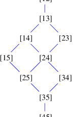
Figure 1. Young’s poset for $(m,p)=(3,2)$.

Fix any linear ordering on the variables in $S$ which refines the ordering in Young’s poset, and let $\prec$ denote the induced degree reverse lexicographic term order on $S$. Let $I_{m,p}$ be the ideal of polynomials in $S$ which vanish on the Grassmannian, that is, $I_{m,p}$ is the ideal of algebraic relations among the maximal minors of a generic $(m+p)\times p$-matrix $X$. The Gröbner homotopy is based on the following well-known result.

Proposition 2.1.

The initial ideal $\,in_{\prec}(I_{m,p})\,$ is generated by all quadratic monomials $\,[\,\alpha\,][\,\beta\,]\,$ where $\alpha_{i}<\beta_{i}$ and $\alpha_{j}>\beta_{j}\,$ for some $i,j\in\{1,\ldots,p\}$.

In other words, $\,in_{\prec}(I_{m,p})\,$ is generated by products of incomparable pairs in Young’s poset. Let ${\mathcal{C}}_{m,p}$ denote the set of all maximal chains in Young’s poset. For example,

$${\mathcal{C}}_{3,2} = \left\{\,\{[12],[13],[14],[15],[25],[35],[45]\}\,,\,\,\{[12],[13],[14],[24],[25],[35],[45]\}\,,\right.$$

$$\hskip 6.6pt\{[12],[13],[14],[24],[34],[35],[45]\}\,,\,\,\{[12],[13],[23],[24],[34],[35],[45]\}\,,$$

$$\hskip 5.2pt\left.\{[12],[13],[23],[24],[25],[35],[45]\}\,\right\}$$

A standard result in combinatorics [36] states that the cardinality of ${\mathcal{C}}_{m,p}$ equals the number (3). From Proposition 2.1 we read off the following prime decomposition which generalizes (8):

(10) $$in_{\prec}(I_{m,p})\quad=\quad\bigcap_{C\in{\mathcal{C}}_{m,p}}\langle\,\,[\alpha]\,\,:\,\,[\alpha]\not\in C\,\rangle.$$

For a proof of Proposition 2.1 see [16, §XIV.9] or [6, Theorem (4.3)] or [38, §3.1]. In these references one finds an explicit minimal Gröbner basis for $I_{m,p}$, which is classically called the set of straightening syzygies. In the special case $p=2$ the straightening syzygies coincide with the reduced Gröbner basis:

Proposition 2.2.

If $p=2$ then the reduced Gröbner basis of $I_{m,p}$ consists of the three-term Plücker relations $\,\underline{[il][kj]}-[ik][jl]+[ij][kl]\,$ where $1\leq i<j<k<l\leq m+p=m+2$.

For $p\geq 3$ the straightening syzygies and the reduced Gröbner basis do not coincide, and they are complicated to describe. For our purposes the following coarse description suffices. Let $Std$ be the set of all quadratic monomials in $S$ which do not lie in $in_{\prec}(I_{m,p})$. The reduced Gröbner basis consists of elements of the form

(11) $$[\alpha][\beta]\quad-\quad\sum_{[\gamma][\delta]\in Std}E^{\alpha,\beta}_{\gamma,\delta}\cdot[\gamma][\delta]$$

where $[\alpha][\beta]$ runs over all generators of $in_{\prec}(I_{m,p})$. The constants $\,E^{\alpha,\beta}_{\gamma,\delta}\,$ are integers which can be computed by substituting (4) into (11) and solving linear equations.

The term order $\prec$ can be realized for the ideal $I_{m,p}$ by the following choices of weights. We define the weight of the variable $[\alpha]=[\alpha_{1}\alpha_{2}\cdots\alpha_{p}]$ to be

(12) $$v_{\alpha}\quad:=\quad-\frac{1}{2}\sum_{1\leq i<j\leq p}(\alpha_{j}-\alpha_{i}-1)^{2}.$$

If we replace each variable $\,[\alpha]\,$ in (11) by $\,[\alpha]\cdot t^{v_{\alpha}}\,$ and clear $t$-denominators afterwards, then we get the Gröbner homotopy:

$({\text{<a href="\#S2.E11" title="In 2.2. Gröbner homotopy ‣ 2. Linear equations in Plücker coordinates ‣ Numerical Schubert Calculus" class="ltx\_ref ltx\_font\_italic"><span class="ltx\_text ltx\_ref\_tag">11</span></a>}}^{\prime })$ $$[\alpha][\beta]\quad-\quad\sum_{[\gamma][\delta]\in Std}E^{\alpha,\beta}_{\gamma,\delta}\cdot[\gamma][\delta]\cdot t^{v_{\gamma}+v_{\delta}-v_{\alpha}-v_{\beta}}$$

It can be checked that all exponents $v_{\gamma}+v_{\delta}-v_{\alpha}-v_{\beta}$ appearing here are positive integers. The special case $(m,p)=(3,2)$ is presented in (6^′).

In the Gröbner homotopy algorithm, we first solve systems of $mp$ linear equations, one for each chain $C\in{\mathcal{C}}_{m,p}$. These systems consist of the $mp$ equations (5), one for each $K_{i}$, and the $\binom{m+p}{p}-mp-1$ equations

$$[\alpha]\qquad\mbox{for}\qquad[\alpha]\not\in C,$$

suggested by the prime decomposition (10). Once this is accomplished, we trace each of these $d$ solutions from $t=0$ to $t=1$ in the Gröbner homotopy (6^′).

Clearly, the weights $v_{\alpha}$ of (12) are not best possible for any specific value of $m$ and $p$. Smaller weights can be found using Linear Programming, as explained e.g. in the proof of [39, Proposition 1.11]. Another method would be to adapt the “dynamic” approach in [40] to our situation. This is possible since the Gröbner basis in (11) is reverse lexicographic: first deform the lowest variable to zero, then deform the second lowest variable to zero, then the third lowest variable, and so on.

2.3. SAGBI homotopy

Let $X=(x_{ij})$ be an $(m+p)\times p$-matrix of indeterminates. We identify the coordinate ring of the Grassmannian with the ${\bf C}$-algebra generated by the $p\times p$-minors of $X$. Call this algebra $R$ and write $[\alpha](x_{ij})$ for the minor indexed by $\alpha$. Reinterpreting classical results in [16, §XIV.9], it was shown in [38, Theorem 3.2.9] that these generators form a SAGBI basis with respect to the lexicographic term order induced from $\,x_{11}>x_{12}>\cdots>x_{1p}>x_{21}>\cdots>x_{m+p,p}$. This means that the initial algebra ${\bf C}[\,in_{>}(f)\,:\,f\in R\,]\,$ is generated by the main diagonal terms of the $p\times p$-minors,

(13) $${\it in}_{>}\bigl{(}[\alpha](x_{ij})\bigr{)}\quad=\quad x_{\alpha_{1},1}\,x_{\alpha_{2},2}\,x_{\alpha_{3},3}\cdots\cdots x_{\alpha_{m},m}.$$

The resulting flat deformation can be realized by replacing $x_{ij}$ with $\,x_{ij}t^{(i-1)(p-j)}\,$ for $t\rightarrow 0$ in the matrix $X$. If we expand $\,[\alpha](x_{ij}t^{(i-1)(p-j)})\,$ as a polynomial in $t$, then the lowest term equals $t^{w_{a}}$ times the main diagonal monomial (13), where

$$w_{\alpha}\quad:=\quad\sum_{j=1}^{p}\,(\alpha_{j}-1)(p-j).$$

In what follows we multiply that polynomial by $\,t^{-w_{\alpha}}$. For any $t\in{\bf C}$ consider the algebra

$$R_{t}\quad:=\quad{\bf C}\left[\,\,t^{-w_{\alpha}}\cdot[\alpha](x_{ij}t^{(i-1)(p-j)})\,\,:\,\ \alpha\in{\textstyle\binom{[m+p]}{p}}\,\right].$$

Then $R_{1}$ is the coordinate ring of the Grassmannian, and $\,R_{0}\,$ is the algebra generated by the monomials (13). This is a flat deformation of ${\bf C}$-algebras; see [10] and [39, §11].

The SAGBI homotopy is the following system of $mp$ equations:

(14) $$\sum_{\alpha\in\binom{[m+p]}{p}}C^{i}_{\alpha}\cdot t^{-w_{\alpha}}\cdot[\alpha](x_{ij}t^{(i-1)(p-j)})\quad=\quad 0\quad\qquad(i=1,\ldots,mp).$$

We reduce the number of variables to $mp$ by introducing local coordinates as follows: $\,x_{ii}=1\,$ for $i=1,\ldots,p$ and $\,x_{ij}=0\,$ for $i<j$ or $i>m+j$. Our original problem is to solve the system (14) for $t=1$.

The flatness of the family of algebras $R_{t}$ guarantees that the system (14) has the same finite number of complex solutions (counting multiplicities) for almost every $t\in{\bf C}$. For $t=0$ we get a system of linear equations in $R_{0}$:

(15) $$\sum_{\alpha\in\binom{[m+p]}{p}}C^{i}_{\alpha}\cdot x_{\alpha_{1},1}x_{\alpha_{2},2}x_{\alpha_{3},3}\cdots x_{\alpha_{p},p}\quad\qquad(i=1,\ldots,mp).$$

In order to solve these equations we apply the symbolic-numeric algorithm in [17], while taking advantage of the following combinatorial structures described in [39, Remark 11.11]. The common Newton polytope of the equations (15) equals the order polytope of the product of an $m$-chain and a $p$-chain (Sturmfels, Remark 11.11). We have the following combinatorial result.

Proposition 2.3.

The following five numbers coincide:

• the right hand side of (3),

• the number of linear extensions of the product of a $m$-chain and a $p$-chain,

• the number of maximal chains in Young’s poset,

• the normalized volume of the order polytope, and

• the number of roots in $({\bf C}^{*})^{mp}$ of a generic system (15).

The equality of (4) and (5) is a special case of Kouchnirenko’s Theorem [21], as all the equations have the same Newton polytope. The order polytope has a distinguished unimodular regular triangulation with simplices indexed by the chains in Young’s poset. This regular triangulation is induced by the system of weights given in (12). We may use these weights to define a numerical homotopy for finding all isolated solutions of (15). Once this is accomplished, we trace these roots from $t=0$ to $t=1$ in the homotopy (14).

3. Special Schubert conditions

We first describe a purely combinatorial method for computing the number $d$ of solution planes. Instead of the algebraic relation (1.2) we shall make use of Young’s poset which was introduced in Section 2.2. A cover $[\alpha]\lessdot[\beta]$ in Young’s poset determines a unique index $j=j(\alpha,\beta)$ for which

$$\alpha_{j}+1\ =\ \beta_{j}\quad\mbox{and}\quad\alpha_{i}\ =\ \beta_{i}\ \ \ \mbox{for}\ \ \ i\neq j.$$

A chain $\,[\alpha^{0}]\lessdot[\alpha^{1}]\lessdot\cdots\lessdot[\alpha^{l}]\,$ in Young’s poset is increasing at $i$ if either $i=1$, or else $i>1$ and $j(\alpha^{i-2},\alpha^{i-1})\leq j(\alpha^{i-1},\alpha^{i})$. For instance, $[12]\lessdot[13]\lessdot[14]\lessdot[24]$ is increasing at 1 and 2, but decreasing at 3.

Given positive integers $r_{0},\ldots,r_{a}$, the Pieri tree ${\mathcal{T}}(r_{0},\ldots,r_{a})$ consists of all chains of length $r_{0}+\cdots+r_{a}$ in Young’s poset which start at the bottom element $[1,2,\ldots,p]$ and which increase everywhere, except possibly at $r_{0}+1,r_{0}+r_{1}+1,\ldots,r_{0}+\cdots+r_{a-1}+1$. Here we include all initial segments of such chains and we order the chains by inclusion. Label a node in the Pieri tree by the endpoint of the chain which that node represents. Then the sequence of labels from the root to that node is the chain which that node represents. For example, here is ${\mathcal{T}}(2,2)$ when $m=5$, $p=2$:

To compute the number $d$, partition the integer sequence $k_{1},\ldots,k_{n}$ into three parts $r_{0},\ldots,r_{a}$, $r^{\prime}_{0},\ldots,r^{\prime}_{a^{\prime}}$, and $q$. Then $d$ is the number of pairs $(R,S)$ where $R$ is a leaf of ${\mathcal{T}}(r_{0},\ldots,r_{a})$, $S$ is a leaf of ${\mathcal{T}}(r^{\prime}_{0},\ldots,r^{\prime}_{a^{\prime}})$, and the endpoints $[\alpha]$ of $R$ and $[\alpha^{\prime}]$ of $S$ satisfy Pieri’s condition:

(16) $$\alpha^{\prime}_{1}\leq m+p+1-\alpha_{p}<\alpha^{\prime}_{2}\leq\cdots<\alpha^{\prime}_{p}\leq m+p+1-\alpha_{1}$$

Call this set of pairs $\mbox{\em Sols}=\mbox{\em Sols}(r_{0},\ldots,r_{a};r^{\prime}_{0},\ldots,r^{\prime}_{a^{\prime}})$.

For instance, $d=6$ for the sequence $2,2,2,2,2$ with $(m,p)=(5,2)$: Of the 9 pairs $(R,S)$ of leaves of ${\mathcal{T}}(2,2)$, only the following 6 satisfy (16): (Here we represent a leaf by its label.)

(17) $$\left\{([25],[34]),\ ([34],[25]),\ ([25],[25]),\ ([25],[16]),\ ([16],[25]),\ ([16],[16])\right\}.$$

This combinatorial rule for the number $d$ gives the same answer as the algebraic rule (1.2) because the Pieri tree and Pieri’s condition (16) encode the structure of the cohomology ring ${\mathcal{A}}_{m,p}$ with respect to its Schur basis $\{S_{\lambda}\mid p\geq\lambda_{1}\geq\cdots\geq\lambda_{p+1}=0\}$; see [25, §I] or [13, §9.4]. Specifically,

$$\prod_{i=0}^{a}h_{r_{i}}\ =\ \sum_{\lambda_{1}+\cdots+\lambda_{p}=r_{0}+\cdots+r_{a}}K_{\lambda,(r_{0},\ldots,r_{a})}\cdot S_{\lambda},$$

where $K_{\lambda,(r_{0},\ldots,r_{a})}$ is the number of leaves in ${\mathcal{T}}(r_{0},\ldots,r_{a})$ with label

$$[\alpha(\lambda)]\quad:=\quad[\lambda_{p}+1,\lambda_{p-1}+2,\ldots,\lambda_{1}+p].$$

The numbers $K_{\lambda,(r_{0},\ldots,r_{a})}$ are called Kostka numbers. In ${\mathcal{A}}_{m,p}$ we calculate

$$\prod_{i=1}^{n}h_{k_{i}} = \left(\prod_{i=0}^{a}h_{r_{i}}\right)\cdot\left(\prod_{j=0}^{a^{\prime}}h_{r^{\prime}_{j}}\right)\cdot h_{q}$$

$$= \sum_{\lambda,\mu}K_{\lambda,(r_{0},\ldots,r_{a})}K_{\mu,(r^{\prime}_{0},\ldots,r^{\prime}_{a^{\prime}})}\cdot S_{\lambda}\cdot S_{\mu}\cdot h_{q}.$$

We evaluate this expression with Pieri’s formula (Proposition 3.1 below): If $\lambda_{1}+\cdots+\lambda_{p}+\mu_{1}+\cdots+\mu_{p}+q=mp$, then $S_{\lambda}\cdot S_{\mu}\cdot h_{q}$ is either $(h_{m})^{p}$ or 0 depending upon whether or not

$({\text{<a href="\#S3.E16" title="In 3. Special Schubert conditions ‣ Numerical Schubert Calculus" class="ltx\_ref ltx\_font\_italic"><span class="ltx\_text ltx\_ref\_tag">16</span></a>}}^{\prime })$ $$\lambda_{p}\leq m-\mu_{1}\leq\lambda_{2}\leq\cdots\leq\lambda_{1}\leq m-\mu_{p}.$$

The condition (16^′) is equivalent to (16) under the transformation $\,\lambda\leftrightarrow[\alpha(\lambda)]$.

These methods correctly enumerate the $p$-planes which meet each $K_{1},\ldots,K_{n}$ nontrivially because, under the isomorphism between ${\mathcal{A}}_{m,p}$ and the cohomology ring of $\mbox{\em Grass}(p,m+p)$, the indeterminate $h_{k_{i}}$ corresponds to the cohomology class Poincaré dual to $\Omega_{K_{i}}$, the set of $p$-planes which meet $K_{i}$ nontrivially. Moreover, $(h_{m})^{p}$ represents the class dual to a point. The Pieri tree models certain intrinsic deformations (described in §3.3 and §3.5) of the Grassmannian which establish this isomorphism, and which we shall use for computing the $p$-planes which meet each $K_{1},\ldots,K_{n}$ nontrivially.

3.1. Basics on Schubert varieties

For vectors $f_{1},\ldots,f_{j}$ in ${\bf C}^{m+p}$, let $\langle f_{1},\ldots,f_{j}\rangle$ be their linear span. Fix the columns $e_{1},\ldots,e_{m+p}$ of the identity matrix as a standard basis for ${\bf C}^{m+p}$. For $\alpha\in\binom{[m+p]}{p}$, define $\alpha^{\vee}\in\binom{[m+p]}{p}$ by $\alpha^{\vee}_{j}:=m+p+1-\alpha_{p+1-j}$.

A sequence $\alpha\in\binom{[m+p]}{p}$ determines a Schubert variety

$$\Omega_{\alpha}\quad:=\quad\{X\in\mbox{\em Grass}(p,m+p)\,\,\mid\,\,\dim X\cap\langle e_{1},\ldots,e_{\alpha^{\vee}_{j}}\rangle\geq j\,\,\,\hbox{for}\,\,1\leq j\leq p\}.$$

This variety has complex codimension $|\alpha|:=\alpha_{1}-1+\alpha_{2}-2+\cdots+\alpha_{p}-p$. Similarly define

$$\Omega^{\prime}_{\alpha}\quad:=\quad\{X\in\mbox{\em Grass}(p,m+p)\,\,\mid\,\,\dim X\cap\langle e_{\alpha_{j}},\ldots,e_{m+p}\rangle\geq p+1-j\,\,\,\,\hbox{for}\,\,1\leq j\leq p\}.$$

For a linear subspace $N$ of ${\bf C}^{m+p}$ of dimension $m+1-q$, define the special Schubert variety

$$\Omega_{N}\quad:=\quad\{X\in\mbox{\em Grass}(p,m+p)\,\,\mid\,\,\dim X\cap N\geq 1\}.$$

This has codimension $q$. If $N=\langle e_{1},\ldots,e_{m+1-q}\rangle$, then $\Omega_{N}=\Omega_{[1,\ldots,p-1,p+q]}$.

The special Schubert variety $\Omega_{N}$ is cut out by the system of $\binom{m+p}{q-1}$ polynomial equations:

(18) $$X\ \in\ \Omega_{N}\quad\Longleftrightarrow\quad\mbox{all maximal minors of }\left[X\mid N\right]\,\mbox{are zero,}$$

where $X\in\mbox{\em Grass}(p,m+p)$ is represented by a $(m+p)\times p$-matrix. The Laplace expansion of these equations in terms of the Plücker coordinates of $X$ define $\Omega_{N}$ as a subscheme of $\mbox{\em Grass}(p,m+p)$. These equations are redundant: select $m\!+\!1\!-\!q$ rows of $\left[X\mid N\right]$ such that the corresponding maximal minor of $N$ is invertible. Consider the set of maximal minors of $\left[X\mid N\right]$ which cover all the rows selected. This gives $\binom{p}{q-1}$ polynomial equations which generate the same ideal as all $\binom{m+p}{q-1}$ minors of $\left[X\mid N\right]$. For a purely set-theoretic (but not scheme-theoretic) representation of $\Omega_{N}$ a further substantial reduction in the number of equations is possible using the results of [5].

An intersection $Y\cap Z$ of subvarieties is generically transverse if every component of $Y\cap Z$ has an open subset along which $Y$ and $Z$ meet transversally. In this case the following identity in the cohomology ring holds:

$$[Y\cap Z]\quad=\quad[Y]\cdot[Z],$$

where $[W]$ denotes the cycle class of a subvariety $W$. By Kleiman’s Transversality Theorem [19], subvarieties of ${\it Grass}(p,m+p)$ in general position meet generically transversally. Transversality and generic transversality coincide when $Y\cap Z$ is finite.

Proposition 3.1 (Hodge and Pedoe, 1952, Theorem III in §XIV.4).

Let $\alpha,\,\alpha^{\prime}\in\binom{[m+p]}{p}$ with $|\alpha|+|\alpha^{\prime}|+q=mp$ and let $N$ be a linear subspace of ${\bf C}^{m+p}$ with dimension $m+1-q$ none of whose Plücker coordinates vanish. Then the intersection

(19) $$\Omega_{\alpha}\,\cap\,\Omega^{\prime}_{\alpha^{\prime}}\,\cap\,\Omega_{N}$$

either is transverse consisting of a single $p$-plane or is empty, depending upon whether or not (16) holds.

Proof and Algorithm: The intersection $\Omega_{\alpha}\cap\Omega^{\prime}_{\alpha^{\prime}}$ is nonempty if and only if $\alpha^{\prime}_{j}\leq\alpha^{\vee}_{j}$ for $j=1,\ldots,p$. These are the weak inequalities in (16). We shall assume that they hold in what follows. The $p$-planes in $\Omega_{\alpha}\cap\Omega^{\prime}_{\alpha^{\prime}}$ are represented by $(m+p)\times p$-matrices $X=(x_{ij})$ such that

(20) $$x_{i,j}\ =\ 0\qquad\mbox{for}\qquad i<\alpha^{\prime}_{j}\quad\mbox{or}\quad\alpha^{\vee}_{j}<i.$$

Consider the nonzero coordinate subspaces $\,C_{j}:=\langle e_{\alpha^{\prime}_{j}},\ldots,e_{\alpha^{\vee}_{j}}\rangle$, set $\,C:=C_{1}+\cdots+C_{p}$, and note that $\,p+q=\sum_{j}\dim(C_{j})\geq dim(C)$. From (20) we see that $\,X\in\Omega_{\alpha}\cap\Omega^{\prime}_{\alpha^{\prime}}\,$ implies $\,X\subseteq C\,$ and hence $\,N\cap X\subseteq N\cap C$. Therefore the triple intersection (19) is nonempty only if the following equivalent conditions hold:

$$dim(C\cap N)\geq 1\,\,\iff\,\,dim(C)=p+q\,\,\iff\,\mbox{the sum}\,\,\,C=C_{1}+\cdots+C_{p}\,\,\,\mbox{is direct}$$

$$\iff\,\alpha^{\vee}_{j}<\alpha^{\prime}_{j+1}\,\,\mbox{for}\,\,j=1,\ldots,p-1\,\iff\,\mbox{(3.1) holds.}$$

In this case we determine$\,C\cap N\,$ by computing vectors $\,g_{j}\in C_{j}\,$ such that $\,C\cap N=\langle g_{1}\oplus g_{2}\oplus\cdots\oplus g_{p}\rangle$. (This computation is the “algorithm” part in this proof.) The desired $p$-plane $X$ satisfies $\,C\cap N=X\cap N$, and, in view of (20), this implies $X=\langle g_{1},\ldots,g_{p}\rangle$. Transversality of (19) is verified in local coordinates for $\Omega_{\alpha}\cap\Omega^{\prime}_{\alpha^{\prime}}$ by considering $p+q-1$ independent linear forms which vanish on $N$.∎

For $\alpha\in\binom{[m+p]}{m}$ define $\lambda(\alpha)$ by $\lambda(\alpha)_{j}:=\alpha_{j}-j$ for $1\leq j\leq p$. Then $S_{\lambda(\alpha)}$ represents the cycle class of $\Omega_{\alpha}$ (equivalently, of $\Omega^{\prime}_{\alpha}$). If $\dim N=m+1-q$, then $h_{q}$ is the cycle class of $\Omega_{N}$. Suppose $|\alpha|+|\alpha^{\prime}|+q=mp$. Then Proposition 3.1 implies the following identity in ${\mathcal{A}}_{m,p}$:

$$S_{\lambda(\alpha)}\cdot S_{\lambda(\alpha^{\prime})}\cdot h_{q}\ =\ \left\{\begin{array}[]{cl}(h_{m})^{p}&\quad\mbox{if }(\ref{eq:pieri})\mbox{ holds}\\ 0&\quad\mbox{otherwise}\end{array}\right..$$

This identity implies (via Poincaré duality) that

$$S_{\lambda(\alpha)}\cdot h_{q}\quad=\quad\sum S_{\lambda(\beta)},$$

the sum over all $\beta$ with $|\beta|=|\alpha|+q$ for which $\alpha,\beta^{\vee}$ satisfy Pieri’s condition (16). Call this set $\alpha*q$, which is also the set of endpoints of increasing chains of length $q$ in Young’s poset that begin at $\alpha$.

This last form has geometric content. In [35], explicit deformations were given that transform the irreducible intersection $\Omega_{\alpha}\cap\Omega_{N}$ into the cycle $\sum_{\beta\in\alpha*q}\Omega_{\beta}$. Moreover, the branching of the components of the cycles in these deformations reflects the branching among these increasing chains above $\alpha$. This process may be iterated to transform an intersection of several special Schubert varieties into a sum of triple intersections of the form (19), indexed by pairs $(R,S)\in\mbox{\em Sols}$. From this sum, we obtain a set of start solutions indexed by Sols. Also, every intermediate cycle in these deformations consists of the same number (counting multiplicities) of $p$-planes. The Pieri homotopy begins with one of the start solutions and uses numerical path continuation to trace the sequence of curves defined by these deformations which connect that start solution to a solution of the original problem.

3.2. Pieri homotopy algorithm

Given linear subspaces $K_{1},\ldots,K_{n}$ in general position with $\dim K_{i}=m+1-k_{i}$ and $k_{1}+\ldots+k_{n}=mp$, first partition $K_{1},\ldots,K_{n}$ into three lists:

$$L_{0},\ldots,L_{a},\qquad L^{\prime}_{0},\ldots,L^{\prime}_{a^{\prime}},\qquad N$$

where $\dim L_{i}=m+1-r_{i}$, $\dim L^{\prime}_{i}=m+1-r^{\prime}_{i}$, and $\dim N=m+1-q$. Construct the Pieri trees ${\mathcal{T}}(r_{0},\ldots,r_{a})$ and ${\mathcal{T}}(r^{\prime}_{0},\ldots,r^{\prime}_{a^{\prime}})$, and form the set Sols. Change coordinates so that $L_{0}=\langle e_{1},\ldots,e_{m+1-r_{0}}\rangle$ and $L^{\prime}_{0}=\langle e_{p+r^{\prime}_{0}},\ldots,e_{m+p}\rangle$. Set $\tau:=\max\{r_{1}+\cdots+r_{a},\ r^{\prime}_{1}+\cdots+r^{\prime}_{a^{\prime}}\}$.

Given a chain $R$ in the Pieri tree and a positive integer $k$, let $R(k)$ be the $k$th element in that chain, or, if $k$ exceeds the length of $R$, then let $R(k)$ be the endpoint of $R$. For each $(R,S)\in{\it Sols}$ and $k$ from $\tau$ to $0$ we shall construct (in Definition 3.2 below) one-parameter families $Z_{R,k}(t)$ and $Z^{\prime}_{S,k}(t)$ of pure-dimensional subvarieties of ${\it Grass}(p,m+p)$ with the following properties:

1. $Z_{R,k}(t)\subset\Omega_{R(r_{0}+k)}$ and $Z^{\prime}_{S,k}(t)\subset\Omega^{\prime}_{S(r^{\prime}_{0}+k)}$.

2. For $t=0$ or $1$ and each $k$, $Z_{R,k}(t)\cap Z^{\prime}_{S,k}(t)\cap\Omega_{N}$ is transverse and 0-dimensional.

3. $Z_{R,\tau}(t)=\Omega_{R(r_{0}+\tau)}$ and $Z^{\prime}_{S,\tau}(t)=\Omega^{\prime}_{S(r_{0}+\tau)}$ .

4. $Z_{R,k+1}(1)$ is a component of $Z_{R,k}(0)$. Likewise, $Z^{\prime}_{S,k+1}(1)$ is a component of $Z^{\prime}_{S,k}(0)$.

5. $Z_{R,0}(1)=\Omega_{L_{0}}\cap\cdots\cap\Omega_{L_{a}}$ and $Z^{\prime}_{S,0}(1)=\Omega_{L^{\prime}_{0}}\cap\cdots\cap\Omega_{L^{\prime}_{a^{\prime}}}$.

Property 4 is a consequence of Proposition 3.4, the others follow from the assumption of genericity and the definition (Definition 3.2) of the families $Z_{R,k}(t)$ and $Z^{\prime}_{S,k}(t)$.

By 2, the family $W_{(R,S),k}(t)$ over ${\bf C}$ whose fibre at general $t$ (including $t=0$ and $t=1$) is

$$W_{(R,S),k}(t)\quad:=\quad Z_{R,k}(t)\cap Z^{\prime}_{S,k}(t)\cap\Omega_{N}$$

consists of a finite number of curves. In fact, for general $t$ (including $t=0$ and $t=1$), $W_{(R,S),k}(t)$ has the following general form (see Definition 3.2 for the precise form):

$$W_{(R,S),k}(t)\ =\ \Omega_{\alpha}\cap\Omega^{\prime}_{\alpha^{\prime}}\cap\Omega_{M_{1}}\cap\cdots\cap\Omega_{M_{s}},$$

where $M_{1},\ldots,M_{s}$ are linear subspaces with $M_{s}=N$, which depend upon $R,S,k$, the subspaces $L_{1},\ldots,L_{a}$, $L^{\prime}_{1},\ldots,L^{\prime}_{a^{\prime}}$, and at most two of the $M_{i}$ depend upon $t$. Also, $\alpha$ and $\alpha^{\prime}$ depend upon $R,S$, and $k$ with the typical case being $\alpha=R(r_{0}+k)$ and $\alpha^{\prime}=S(r^{\prime}_{0}+k)$.

The numerical homotopy defined by the curves $W_{(R,S),k}(t)$ may be expressed in a parameterization $X=(x_{i,j})$ of an open subset of $\Omega_{\alpha}\cap\Omega^{\prime}_{\alpha^{\prime}}$:

(21) $$x_{i,j}\ =\ 0\qquad\mbox{if}\qquad i<\alpha^{\prime}_{j}\quad\mbox{or}\quad\alpha^{\vee}_{j}<i\quad\qquad\mbox{and}\quad\qquad x_{\delta_{j},\,j}\ =\ 1,$$

where $\delta:=S(r^{\prime}_{0}+\tau)$. The equations for $W_{(R,S),k}(t)$ are then

$$\mbox{maximal minors }\left[X\mid M_{i}\right]\ =\ 0\qquad i=1,\ldots,s.$$

The curves of $W_{(R,S),k}(t)$ define the sequences of homotopies in the Pieri homotopy algorithm as follows: For $(R,S)\in{\it Sols}$, let $X_{(R,S),\tau}$ be the (unique by Proposition 3.1) $p$-plane in $\Omega_{R(r_{0}+\tau)}\cap\Omega^{\prime}_{S(r^{\prime}_{0}+\tau)}\cap\Omega_{N}=W_{(R,S),\tau}(1)$. By 3 and 4, $X_{(R,S),\tau}\in W_{(R,S),\tau-1}(0)$ and hence lies on a unique curve in $W_{(R,S),\tau-1}(t)$. Use numerical path continuation to trace this curve from $t=0$ to $t=1$ to obtain $X_{(R,S),\tau-1}$, which is a point of $W_{(R,S),\tau-2}(0)$, by 4. Then $X_{(R,S),\tau-1}$ lies on a unique curve in $W_{(R,S),\tau-2}(t)$, which we trace to find $X_{(R,S),\tau-2}\in W_{(R,S),\tau-2}(1)$. Continuing this process, after tracing $\tau$ curves, we obtain $X_{(R,S),0}\in W_{(R,S),0}(1)$, which is a solution to the original system, by 5. We show shall prove in Theorem 3.5 that $\{X_{(R,S),0}\mid(R,S)\in{\it Sols}\}$ consists of all the solutions to the original system.

3.3. Definition of the moving cycles $Z_{R,k}(t)$

The cycle $Z_{R,k}(t)$ will depend upon the choice of a general upper triangular $(m+p)\times(m+p)$-matrix $F$ with 1’s on its anti-diagonal,

$$\left(\begin{array}[]{ccc}*&*&1\\ {}*&\hskip 1.0pt\raisebox{0.0pt}{.}\raisebox{2.2pt}{.}\raisebox{4.4pt}{.}\\ 1&&0\end{array}\right),$$

the $k$th link in the chain $R$, and the data $L_{1},\ldots,L_{a}$. The key ingredient of this definition of $Z_{R,k}(t)$ is the construction of a one-parameter family of linear subspaces $\Lambda_{i}(t)$ in Definition 3.3, which depends upon $F$. The matrix $F$ is fixed throughout the algorithm, its purpose is that $\langle e_{m+p-j},\ldots,e_{m+p}\rangle$ equals the span of the first $j$ columns of $F$, and these columns are in general position with $e_{1},\ldots,e_{m+p}$. The subtle linear degeneracies of $\Lambda_{i}(t)$ as $t\rightarrow 0$ are at the heart of this homotopy algorithm, as well as the explicit proof of Pieri’s formula [35, Theorem 3.6], which we state below (Proposition 3.4).

Definition 3.2.

 

1. If $r_{1}+\cdots+r_{a}\leq k$, then set  $Z_{R,k}(t)\ :=\ \Omega_{R(r_{0}+\tau)}$.

2. Otherwise, define $c$ by $r_{1}+\cdots+r_{c-1}\leq k<r_{1}+\cdots+r_{c}$, and set $i:=k-r_{1}-\cdots-r_{c-1}$, $\alpha:=R(r_{0}+r_{1}+\cdots+r_{c-1})$, and $\beta:=R(r_{0}+k)$.

   1. If $i>0$ and $\beta_{p}>\alpha_{p}$, then $\beta+(0,\ldots,0,r_{c}-i)=R(r_{0}+\cdots+r_{c})$, and we set

      $$Z_{R,k}(t)\ :=\ \Omega_{R(r_{0}+\cdots+r_{c})}\cap\Omega_{L_{c+1}}\cap\cdots\cap\Omega_{L_{a}}.$$

   2. Otherwise, let $\Lambda_{i}(t)$ be the 1-parameter family of linear subspaces given by Definition 3.3, where we let $L:=L_{c}$ and $r:=r_{c}$.

      If $i=0$, then $\Lambda_{0}(1)=L_{c}$, $\alpha=\beta=R(r_{0}+k)$, and we set

      $$Z_{R,k}(t)\ :=\ \Omega_{R(r_{0}+k)}\cap\Omega_{\Lambda_{0}(t)}\cap\Omega_{L_{c+1}}\cap\cdots\cap\Omega_{L_{a}}.$$

      If $i>0$, let $j$ be maximal such that $\beta_{j}>\alpha_{j}$. Then $j<p$ as $j=p$ is case 2(a). Set

      $$Z_{R,k}(t)\ :=\ \Omega_{R(r_{0}+k)}\cap\Omega_{\Lambda_{i}(t)\cap\langle e_{1},\ldots,e_{\beta^{\vee}_{p+1-j}}\rangle}\cap\Omega_{L_{c+1}}\cap\cdots\cap\Omega_{L_{a}}.$$

We define $Z^{\prime}_{S,k}(t)$ similarly, but with the matrix $F$ replaced by a lower triangular matrix with 1’s on its diagonal, and $\langle e_{1},\ldots,e_{\beta^{\vee}_{p+1-j}}\rangle$ replaced by $\langle e_{\beta_{j}},\ldots,e_{m+p}\rangle$.

Definition 3.3.

Let $F$ be an upper triangular matrix with 1’s on the anti-diagonal and $L$ be a general $(m+1-r)$-plane, represented as a $(m+p)\times(m+1-r)$-matrix with columns $l_{1},\ldots,l_{m+1-r}$. Construct a $(m+p)\times p$-matrix $U=(u_{1},\ldots,u_{p})$ as follows: Reverse the last $m+p-\alpha_{p}$ columns of $F$, then remove the columns indexed by $\alpha^{\vee}_{1},\ldots,\alpha^{\vee}_{p}$.

For each $0\leq i<r$, define a one-parameter family of $(m+p)\times(m+1-r)$-matrices $\Lambda_{i}(t)$ for $t\in{\bf C}$ as follows:

1. If $i=0$, then the $b$th column of $\Lambda_{0}(t)$ is $t\cdot l_{b}+(1-t)\cdot u_{b}$.

2. For $0<i<r$, the $b$th column of $\Lambda_{i}(t)$ is

   $$\begin{array}[]{lcl}t\cdot u_{b+i-1}+(1-t)\cdot u_{b+i}&&b+i-1<\alpha_{p}-p\\ t\cdot u_{b+i-1}+(1-t)\cdot u_{p+1+i-r}&&b+i-1=\alpha_{p}-p\\ u_{b+i-1}&&b+i-1>\alpha_{p}-p\end{array}$$

3.4. An example

We give an example illustrating these definitions and the Pieri homotopy algorithm. Let $L_{0},L_{1},L^{\prime}_{0},L^{\prime}_{1}$, and $N$ be general 4-planes in ${\bf C}^{7}$. We give a sequence of homotopies $W_{(R,S),k}(t)$ for $k=2,1,0$ for finding one of the six $2$-planes which meet each of the five given 4-planes nontrivially.

Here, $(m,p)=(5,2)$ and $k_{1}=\cdots=k_{5}=2$ so that $\tau=2$. Construct the set Sols as in (17). Let $(R,S)\in\mbox{\em Sols}$ be the following two sequences:

$$R\ :=\ [12]\lessdot[13]\lessdot[14]\lessdot[24]\lessdot[25],\qquad S\ :=\ [12]\lessdot[13]\lessdot[14]\lessdot[15]\lessdot[16].$$

Let $e_{1},\ldots,e_{7}$ be the columns of a $7\times 7$-identity matrix, a basis for ${\bf C}^{7}$. Suppose that $L_{0}=\langle e_{4},e_{5},e_{6},e_{7}\rangle$ and $L^{\prime}_{0}=\langle e_{1},e_{2},e_{3},e_{4}\rangle$ and represent $L_{1}$ and $L^{\prime}_{1}$ as $7\times 4$-matrices. Then $\Omega_{[14]}\cap\Omega_{L}\cap\Omega^{\prime}_{[14]}\cap\Omega_{L^{\prime}}\cap\Omega_{N}$ is the set of 2-planes which meet all five linear subspaces nontrivially.

We first find the plane $X_{(R,S),2}\in\Omega_{[25]}\cap\Omega^{\prime}_{[16]}\cap\Omega_{N}$, using the algorithm in the proof of Proposition 3.1. Suppose that $N$ has the form

$$\left[\begin{array}[]{c}n\\ \hline\cr I\end{array}\right],$$

where $I$ is the $4\times 4$ identity matrix, and $n$ is a $3\times 4$-matrix. In this case, $C_{1}=\langle e_{1},e_{2},e_{3}\rangle$ and $C_{2}=\langle e_{6}\rangle$, hence $C=\langle e_{1},e_{2},e_{3},e_{6}\rangle$. Thus the intersection $C\cap N$ is generated by the third column of $N$, and so $X_{(R,S),2}$ is represented by the matrix:

$$X_{(R,S),2}\quad=\quad\left[\begin{array}[]{cc}n_{13}&0\\ n_{23}&0\\ n_{33}&0\\ 0&0\\ 0&0\\ 0&1\\ 0&0\\ \end{array}\right].$$

Following Definition 3.3, we have:

$$\Lambda_{0}(t) = \langle tl_{1}+(1-t)u_{1},tl_{2}+(1-t)u_{2},tl_{3}+(1-t)u_{3},tl_{4}+(1-t)u_{4}\rangle,$$

$$\Lambda_{1}(t) = \langle tu_{1}+(1-t)u_{2},tu_{2}+(1-t)u_{5},u_{3},u_{4}\rangle.$$

$\Lambda^{\prime}_{i}(t)$ is defined similarly.

We describe the families $W_{(R,S),k}(t)$ for $k=2,1,0$ in local coordinates for $\Omega_{[14]}\cap\Omega^{\prime}_{[14]}$ determined by the sequence $[16]$:

$$X\quad=\quad\left[\begin{array}[]{cc}1&0\\ x_{21}&0\\ x_{31}&0\\ x_{41}&x_{42}\\ 0&x_{52}\\ 0&1\\ 0&x_{72}\\ \end{array}\right]\ .$$

The family $W_{(R,S),2}(t)$ is the constant family $\{X_{(R,S),2}\}=\Omega_{25}\cap\Omega^{\prime}_{16}\cap\Omega_{N}$. Assuming that $n_{13}$, which is the $[1457]$th Plücker coordinate of $N$, is non-zero, then $X_{(R,S),2}$ may be expressed in these local coordinates:

$$X_{(R,S),2}\quad=\quad\left[\begin{array}[]{cc}1&0\\ n_{23}/n_{13}&0\\ n_{33}/n_{13}&0\\ 0&0\\ 0&0\\ 0&1\\ 0&0\\ \end{array}\right]\ .$$

When $k=1$, first consider the definition of $Z_{R,1}(t)$. Here we are in case 2(b) with $\beta=[24]$ and $i>0$, so that $\beta^{\vee}=[46]$. Since $\Lambda_{1}(t)\subset\langle e_{1},\ldots,e_{6}\rangle$, we have $Z_{R,1}(t)\ =\ \Omega_{[24]}\cap\Omega_{\Lambda_{1}(t)}$. For the definition of $Z^{\prime}_{S,1}(t)$, we are in case 2(a), so that $Z^{\prime}_{S,1}(t)\ =\ \Omega^{\prime}_{[16]}$. Hence

$$W_{(R,S),1}(t)\ =\ \Omega_{[24]}\cap\Omega_{\Lambda_{1}(t)}\cap\Omega^{\prime}_{[16]}\cap\Omega_{N}.$$

This has 3 linear equations $x_{42}=x_{52}=x_{72}=0$, which describe $\Omega_{[24]}\cap\Omega^{\prime}_{[16]}$, and 7 non-trivial equations, the vanishing of the maximal minors of $[X\mid\Lambda_{1}(t)]$ and $[X\mid N]$, which describe $\Omega_{\Lambda_{1}(t)}\cap\Omega_{N}$.

For $k=0$, $i=0$ and we are in case 2(b) for both $Z_{R,0}(t)$ and $Z^{\prime}_{S,0}(t)$ so that

$$W_{(R,S),0}(t)\ =\ \Omega_{[14]}\cap\Omega_{\Lambda_{0}(t)}\cap\Omega^{\prime}_{[14]}\cap\Omega_{\Lambda^{\prime}_{0}(t)}\cap\Omega_{N}.$$

This has 21 non-trivial equations, the vanishing of the maximal minors of $\left[X\mid\Lambda_{0}(t)\right]$, $\left[X\mid\Lambda^{\prime}_{0}(t)\right]$, and $\left[X\mid N\right]$.

3.5. Proof of correctness

We describe the Pieri deformations linking the families $Z_{R,k}(t)$ for $k$ from $r_{1}\!+\!\cdots\!+\!r_{c-1}$ to $r_{1}+\cdots+r_{c}$, which establishes Property 4 of $Z_{R,k}(t)$ in §3.2. We also show that the set $\{X_{(R,S),0}\mid(R,S)\in{\it Sols}\}$ consists of all the solutions to the original system.

Consider the dynamic part of $Z_{R,k}(t)$, namely whichever of

$$\Omega_{R(r_{0}+\cdots+r_{c})},\quad\Omega_{R(r_{0}+k)}\cap\Omega_{\Lambda_{0}(t)},\quad\mbox{or}\quad\Omega_{R(r_{0}+k)}\cap\Omega_{\Lambda_{i}(t)\cap\langle e_{1},\ldots,e_{\beta^{\vee}_{p+1-j}}\rangle},$$

appeared in the definition of $Z_{R,k}(t)$. We call this cycle $Y_{\alpha,\beta,L}(t)$, where $L:=L_{c}$ and $\alpha=R(r_{0}+\cdots+r_{c-1})$, and $\beta=R(r_{0}+k)$.

For $\beta\in\alpha*i$ and $\gamma\in\alpha*(i+1)$ write $\beta\prec_{\alpha}\gamma$ if $\gamma$ covers $\beta$ and $j(\beta,\gamma)\geq j(\alpha,\beta):=\max\{j\mid\beta_{j}>\alpha_{j}\}$. This partitions $\alpha*(i+1)$ into sets $\{\gamma\mid\beta\prec_{\alpha}\gamma\}$ for $\beta\in\alpha*i$.

Proposition 3.4.

[35, Theorem 3.6]

Let $\alpha,\beta,i,r,L,\Lambda_{i}(t)$, and $Y_{\alpha,\beta,L}(t)$ be as above. Then

1. For all $t$, $\Omega_{\alpha}\cap\Omega_{\Lambda_{0}(t)}$ is generically transverse.

2. $Y_{\alpha,\beta,L}(t)$ is free of multiplicities for all $t$ and irreducible for $t\neq 0$.

3. If $i\neq r-1$, then $Y_{\alpha,\beta,L}(0)=\sum_{\beta\prec_{\alpha}\gamma}Y_{\alpha,\gamma,L}(1)$.

4. If $\beta\in\alpha*(r-1)$, then $Y_{\alpha,\beta,L}(0)=\sum_{\beta\prec_{\alpha}\gamma}\Omega_{\gamma}$.

By 3, the cycle class of $\sum_{\beta\in\alpha*i}Y_{\alpha,\beta,L}(t)$ is independent of $i$ and $t$, and it equals the cycle class of $\Omega_{\alpha}\cap\Omega_{\Lambda_{0}(1)}=\Omega_{\alpha}\cap\Omega_{L}$. By 4, we see that the cycle classes of $\Omega_{\alpha}\cap\Omega_{L}$ and $\sum_{\beta\in\alpha*r}\Omega_{\beta}$ coincide, furnishing another proof of Pieri’s formula. Property 4 of $Z_{R,k}(t)$ follows from assertion 3.

Theorem 3.5.

When $K_{1},\ldots,K_{n}$ are generic, the Pieri homotopy algorithm finds all $p$-planes which meet each $K_{1},\ldots,K_{n}$ nontrivially. That is,

$$\{X_{(R,S),0}\mid(R,S)\in{\it Sols}\}\quad=\quad\Omega_{K_{1}}\cap\cdots\cap\Omega_{K_{n}}.$$

Proof. Note that for any $R,S\in{\it Sols}$, the families $Z_{R,k}(t),Z^{\prime}_{S,k}(t)$, and $W_{(R,S),k}(t)$ depend only upon the initial segments $R(0),\ldots,R(r_{0}+k)$ and $S(0),\ldots,S(r^{\prime}_{0}+k)$ of $R$ and $S$.

By construction, the original system $\Omega_{K_{1}}\cap\cdots\cap\Omega_{K_{l}}$ coincides with $W_{(R,S),0}(1)$, for any $(R,S)\in\mbox{\em Sols}$. We inductively construct chains $R\in{\mathcal{T}}(r_{0},\ldots,r_{a})$ and $S\in{\mathcal{T}}(r^{\prime}_{0},\ldots,r^{\prime}_{a^{\prime}})$, and $p$-planes $X_{k}$ for $0\leq k\leq\tau$ such that

$$X_{k+1}\ \in\ W_{(R,S),k}(0)\cap W_{(R,S),k+1}(1)$$

and $X_{k},X_{k+1}$ lie on the same curve of $W_{(R,S),k}(t)$. Then $X_{\tau}$ is the start solution $X_{(R,S),\tau}$, which shows that $X_{0}\in\{X_{(R,S),0}\mid(R,S)\in{\it Sols}\}$.

First set $R(0),\ldots,R(r_{0})$ to be the unique chain from $[1,\ldots,p]$ to $[1,\ldots,p-1,p+r_{0}]$, and similarly for $S(0),\ldots,S(r^{\prime}_{0})$. Then $X_{0}\in W_{(R,S),0}(1)$ and hence lies on a unique curve in $W_{(R,S),0}(t)$. Let $X_{1}$ be the point on that curve with $t=0$. By Proposition 3.4 (4),

$$X_{1}\ \in\ Y_{(R(r_{0}),R(r_{0}),L_{1})}(0)\ =\ \sum_{\beta\in R(r_{0})*1}Y_{(R(r_{0}),\beta,L_{1})}(1).$$

Let $R(r_{0}+1)$ be the index $\beta$ such that $X_{1}\in Y_{(R(r_{0}),\beta,L_{1})}(1)$. Define $S(r^{\prime}_{0}+1)$ similarly. Then $X_{1}\in W_{(R,S),1}(1)$.

In general, suppose that we have constructed $R(0),\ldots,R(r_{0}+k)$, $S(0),\ldots,S(r^{\prime}_{0}+k)$, and $X_{k}\in W_{(R,S),k}(1)$. Then $X_{k}$ lies on a unique curve in $W_{(R,S),k}(t)$. Let $X_{k+1}$ be the point on that curve at $t=0$. Let $c$ be minimal subject to $k<r_{1}+\cdots+r_{c}$ and set $\alpha=R(r_{0}+\cdots+r_{c-1})$ and $\beta=R(r_{0}+k)$. If $k+1<r_{1}+\cdots+r_{c}$, then by Proposition 3.4 (3), there is a unique index $\gamma\in\beta*1$ such that $X_{k+1}\in Y_{\alpha,\gamma,L_{c}}(1)$. If $k+1=r_{1}+\cdots+r_{c}$ then by Proposition 3.4 (4), there is a unique index $\gamma\in\beta*1$ such that $X_{k+1}\in\Omega_{\gamma}$. Set $R(r_{0}+k+1)=\gamma$ and likewise define $S(r^{\prime}_{0}+k+1)$. Continuing in this fashion, we construct the chains $R$ and $S$, and $X_{j}$ for $0\leq j\leq\tau$.

We show that $R$ increases everywhere, except possibly at $1,r_{0}+1,\ldots,r_{0}+\cdots+r_{a-1}+1$, and hence $R\in{\mathcal{T}}(r_{0},\ldots,r_{a})$. Similar arguments show that $S\in{\mathcal{T}}(r^{\prime}_{0},\ldots,r^{\prime}_{a^{\prime}})$, which will complete the proof. Suppose $k+1\not\in\{1,r_{1}+1,\ldots,r_{1}+\cdots+r_{a-1}+1\}$. Let $c$ be minimal subject to $k<r_{1}+\cdots+r_{c}$ and let $\alpha=R(r_{0}+\cdots+r_{c-1})$, $\beta=R(r_{0}+k)$, and $\gamma=R(r_{0}+k+1)$. Then by Proposition 3.4 (3) and (4), $\beta\prec_{\alpha}\gamma$. The condition $j(\beta,\gamma)\geq j(\alpha,\beta)$ in the definition of $\beta\prec_{\alpha}\gamma$ ensures that $R$ increases at $k+1$. ∎

4. Homotopy continuation of overdetermined systems

Numerical homotopy continuation is a method for finding the isolated solutions of a system

(22) $$F(X)\ =\ 0$$

where $F=(f_{1},\ldots,f_{n})$ are polynomials in the variables $X=(x_{1},\ldots,x_{N})$. First, a homotopy $H(X,t)$ is found with the following properties:

1. $H(X,1)=F(X)$.

2. The isolated solutions of $H(X,0)=0$ are known.

3. The system $H(X,t)=0$ defines finitely many (rational) curves $\sigma_{i}(t)$, and each isolated solution of (22) is connected to an isolated solution $\sigma_{i}(0)$ of $H(X,0)=0$ by one of these curves.

Given such a homotopy, numerical path continuation is used to trace these curves from solutions of $H(X,0)=0$ to solutions of the original system (22). When there are fewer solutions to $F(X)=0$ than to $H(X,0)=0$, some curves will diverge or become singular as $t\rightarrow 1$, and it is expensive to trace such a curve.

When $N=n$, the system (22) is square and the homotopy

(23) $$H(X,t)\quad:=\quad tF(X)\ +\ (1-t)G(X),$$

where $G(X)=(x_{1}^{d_{1}}-a_{1},\ldots,x_{N}^{d_{N}}-a_{N})$ with $d_{i}:=\deg(f_{i})$ and $a_{i}\neq 0$, gives $\prod d_{i}$ curves. This is the Bézout bound for a generic dense system $F$.

In practice, $F(X)=0$ may have fewer than $\prod d_{i}$ solutions and we desire a homotopy with no divergent curves. Methods for such deficient systems which reduce the number of divergent curves are developed in [23, 22, 24]. When the polynomials $f_{1},\ldots,f_{n}$ have special forms [27, 28], then such homotopies (23) are constructed where $G(X)$ shares this special form. When the polynomials $f_{1},\ldots,f_{n}$ are sparse, polyhedral methods [41, 17] give a homotopy. The SAGBI homotopy algorithm (§2.3) is in the same spirit. We exploit a special feature of the coordinate ring of the Grassmannian to obtain a homotopy between the system (2.2) we wish to solve and one (2.12) whose solution may be obtained using polyhedral methods. Moreover, there are generically no divergent curves to be followed.

The overdetermined situation of $n>N$ is more delicate. One difficulty is finding a homotopy $H(X,t)$ for an overdetermined system as generic perturbations of $F$ have no solutions. In [32, §2], this difficulty is avoided as follows: The system $F=(f_{1},\ldots,f_{n})$ is replaced by $N$ random linear combinations of the $f_{1},\ldots,f_{n}$ yielding a square system whose isolated solutions include all isolated solutions of $F(X)=0$, but typically many more. They then find all isolated solutions of this random square subsystem.

For the Gröbner and Pieri homotopy algorithms, we gave (in §§2.2 and 3.2–3) homotopies $H(X,t)=(h_{1}(X,t),\ldots,h_{n}(X,t))$ and solutions $\sigma_{i}(0)$ at $t=0$ as above. For these, there are generically no divergent curves. To efficiently follow the curves $\sigma_{i}(t)$, we select a square subsystem $MH(X,t)$ of $H(X,t)$ ($M$ is an $(N\times n)$-matrix). If the Jacobian of $MH$ at each $\sigma_{i}(0)$ has the same rank ($N$) as does the Jacobian of $H(X,t)$, then the curves $\sigma_{i}(t)$ remain components of the algebraic set defined by the equations

$$MH(X,t)\ =\ 0.$$

Moreover, other components of this set meet the curves $\sigma_{i}(t)$ in at most finitely many points $t$ in ${\bf C}-\{0\}$. Thus, we may use the square subsystem $MH(X,t)$ to trace the curves $\sigma_{i}(t)$ along some path from 0 to 1 in the complex plane. We remark that in practice, $M$ may be chosen at random.

5. Applications

The algorithms of Sections 2 and 3 are useful for studying both the pole assignment problem in systems theory [8] and real enumerative geometry [33].

We describe the connection to the control of linear systems following [8]. Suppose we have a system (for example, a mechanical linkage) with inputs $u\in{\bf R}^{m}$ and outputs $y\in{\bf R}^{p}$ for which there are internal states $x\in{\bf R}^{n}$ such that the evolution of the system is governed by the first order linear differential equation

(24) $$\begin{array}[]{rcl}\dot{x}&=&Ax+Bu,\\ y&=&Cx.\end{array}$$

If the input is controlled by constant output feedback, $u=Fy$, then we obtain

$$\dot{x}\ =\ (A+BFC)x.$$

The natural frequencies of the controlled system are the roots $s_{1},\ldots,s_{n}$ of

(25) $$\varphi(s)\ :=\ \det(sI-A-BFC).$$

The pole assignment problem asks, given a system (24) and a polynomial $\varphi(s)$ of degree $n$, which feedback laws $F$ satisfy (25)?

A standard transformation (cf. [8, §2]) transforms the input data $A,B,C$ into matrices $N(s)$, $D(s)$ of polynomials with $\det(D(s))=\det(sI-A)$ and $N(s)D(s)^{-1}=C(sI-A)^{-1}B$ such that

(26) $$\varphi(s)\ =\ \det\left[\begin{array}[]{cc}F&D(s)\\ I&N(s)\end{array}\right].$$

Here $I$ is the $p\times p$-identity matrix and the feedback law $F$ is an $m\times p$-matrix. If we let

$$X\ :=\ \left[\begin{array}[]{c}F\\ I\end{array}\right]\qquad{\rm and}\qquad K(s)\ :=\ \left[\begin{array}[]{c}D(s)\\ N(s)\end{array}\right],$$

then $F$ gives local coordinates on $\mbox{\em Grass}(p,m+p)$ and (26) is equivalent to

$$X\cap K(s_{i})\ \neq\ \{0\}\quad\mbox{for}\quad i\ =\ 1,\ldots,n.$$

These conditions are independent for generic $A,B,C$ and distinct $s_{i}$, hence $n\leq mp$ is necessary for there to be any feedback laws $F$. The critical case of $n=mp$ is an instance of the situation in §2.

In [9] homotopy continuation was used to solve a specific feedback problem when $(m,p)=(3,2)$. From this result, they deduced that the pole assignment problem is not in general solvable by radicals. Despite this success, only few non-trivial examples have been computed in the control theory literature [30].

An important question is whether a given system may be controlled by real output feedback [42, 7, 29]. That is, if all roots of $\varphi(s)$ are real, are there real feedback laws $F$ satisfying (26)? Real enumerative geometry [33] asks a similar question: Are there real linear subspaces $K_{1},\ldots,K_{n}$ in general position with $\dim K_{i}=m+1-k_{i}$ and $k_{1}+\cdots+k_{n}=mp$ such that all $p$-planes meeting each $K_{i}$ nontrivially are real? When either $m$ or $p$ is 2 [34], $n\leq 5$ [35], or when $m=p=3$ and the $k_{i}=1$ [33], the answer is yes. In fact, the Pieri homotopies arose from these investigations.

B. Shapiro and M. Shapiro give a precise conjecture relating both applications. Suppose

$$K_{i}(s)\ :=\ [\gamma(s),\gamma^{\prime}(s),\gamma^{\prime\prime}(s),\ldots,\gamma^{(m+1-k_{i})}(s)],$$

where $\gamma(s)$ is a parameterization of a rational normal (non-degenerate) curve in ${\bf R}^{m+p}$ of degree $m+p-1$. One such choice is

(27) $$\gamma(s)\ =\ {\it transpose}[1,s,s^{2},\ldots,s^{m+p-1}].$$

Geometrically, $K_{i}(s)$ is the $(m+1-k_{i})$-plane which osculates the curve $\gamma(s)$ at $s$. Such osculating $m$-planes have been used to prove non-degeneracy results in control theory.

Conjecture 5.1 (B. Shapiro and M. Shapiro).

Let $s_{1},\ldots,s_{n}$ be distinct real numbers and suppose $K_{i}(s_{i})$ osculates $\gamma$ at $s_{i}$ and $k_{1}+\cdots+k_{n}=mp$. Then each of the finitely many $p$-planes $X\subset{\bf C}^{m+p}$ satisfying $X\cap K_{i}(s_{i})\neq\{0\}$ for $i=1,\ldots,n$ is defined over the reals.

6. Computational results

Our algorithms have been tested successfully in MATLAB, finding all 14 solutions in the case $(m,p)=(4,2)$ for both the SABGI and Gröbner homotopy algorithm, and all 15 solutions when $(m,p)=(6,2)$ and $k_{1}=\cdots=k_{6}=2$ for the Pieri homotopy algorithm.

At present, the SAGBI and Gröbner homotopy algorithms have been fully implemented. Some timings from trial runs of these algorithms on a Sparc 20 are displayed in Table 1. The input for these were $mp$ random complex $(m+p)\times m$-matrices.

We provide a comparison to methods based upon Gröbner bases. Table 1 also gives the time on the Sparc 20 for the system Singular [15] to compute a degree reverse lexicographic Gröbner basis for the polynomial systems:

$$\det\left[X\mid K_{i}\right]\ =\ 0,\quad\mbox{for}\quad i=3,\ldots,K_{mp}.$$

Here $X$ is expressed in local coordinates for $\,\Omega_{[13]}\,\cap\,\Omega^{\prime}_{[13]}\,$ and the $K_{3},\ldots,K_{mp}$ are $(m+p)\times m$-matrices with random integral entries between $-4$ and $4$. A degree reverse lexicographic Gröbner basis is the input for some alternative numerical polynomial systems solvers (e.g. eigenvalue methods [3]). We note that the Gröbner basis calculation did not terminate within one week in the case $(m,p)=(6,2)$.

$m$	$p$	$d(m,p)$	SABGI homotopy	Gröbner homotopy	Gröbner basis
3	2	5	${<}1$	$<0.5$	$<0.5$
4	2	14	$47$	$6$	$19$
5	2	42	$373$	$408$	$149,897$
6	2	132	$3,364$	$8,626$	$\infty$

Table 1. Time (in seconds)

The final version of this paper will include data from implementations of the Pieri homotopy algorithm, as well.

References

- [1] E. Allgower and K. Georg, Numerical Continuation Methods, An Introduction, no. 13 in Computational Mathematics, Springer-Verlag, 1990.
- [2] E. Allgower and K. Georg, Numerical path following. To appear in the Handbook of Numerical Analysis, edited by P. G. Ciarles and J.L. Lions, North Holland, 1997.
- [3] W. Auzinger and H. Stetter, An elimination algorithm for the computation of the zeros of a system of multivariate polynomial equations, in Numerical Mathematics, Singapore, 1988, R. Agarwal, Y. Chow, and S. Wilson, eds., vol. 86 of Internat. Schriftenreihe Numer. Math., Birkhäuser, 1988, pp. 11–30.
- [4] D. N. Bernstein, The number of roots of a system of equations, Funct. Anal. Appl., 9 (1975), pp. 183–185.
- [5] W. Bruns and R. Schwänzl, The number of equations defining a determinantal variety, Bull. London Math. Soc., 22 (1990), pp. 439–445.
- [6] W. Bruns and U. Vetter, Determinantal Rings, Lecture Notes in Math., Vol. 1327, Springer-Verlag, 1988.
- [7] C. I. Byrnes, Control theory, inverse spectral problems, and real algebraic geometry, in Diffferential Geometric Methods in Control Theory, R. W. Brockett, R. S. Millman, and H. J. Sussmann, eds., Birkhäuser, Boston, 1982, pp. 192–208.
- [8] C. I. Byrnes, Pole assignment by output feedback, in Three Decades of Mathematical Systems Theory, H. Nijmeijer and J. M. Schumacher, eds., vol. 135 of Lecture Notes in Control and Inform. Sci., Springer-Verlag, Berlin, 1989, pp. 31–78.
- [9] C. I. Byrnes and P. K. Stevens, Global properties of the root-locus map, in Feedback Control of Linear and Non-Linear Systems, D. Hinrichsen and A. Isidori, eds., vol. 39 of Lecture Notes in Control and Inform. Sci., Springer-Verlag, Berlin, 1982.
- [10] A. Conca, J. Herzog, and G. Valla, Sagbi bases with applications to blow-up algebras, J. reine angew. Math., 474 (1996), pp. 113–138.
- [11] F.-J. Drexler, Eine Methode zur Berechnung sämtlicher Lösungen von Polynomgleichungssystemen, Numer. Math., 29 (1977), pp. 45–58.
- [12] D. Eisenbud, Commutative Algebra With a View Towards Algebraic Geometry, no. 150 in GTM, Springer-Verlag, 1995.
- [13] W. Fulton, Young Tableaux, Cambridge University Press, 1996.
- [14] W. I. García, C. B.; Zangwill, Finding all solutions to polynomial systems and other systems of equations, Math. Programming, 16 (1979), pp. 159–176.
- [15] G.-M. Greuel, G. Pfister, and H. Schönemann, Singular: A system for computation in algebraic geometry and singularity theory. Available via anonymous ftp from helios.mathematik.uni-kl.de, 1996.
- [16] W. V. D. Hodge and D. Pedoe, Methods of Algebraic Geometry, vol. II, Cambridge University Press, 1952.
- [17] B. Huber and B. Sturmfels, A polyhedral method for solving sparse polynomial systems, Math. Comp., 64 (1995), pp. 1541–1555.
- [18] A. Khovanskii, Newton polyhedra and the genus of complete intersections, Funct. Anal. Appl., 12 (1978), pp. 38–46.
- [19] S. Kleiman, The transversality of a general translate, Comp. Math., 28 (1974), pp. 287–297.
- [20] S. Kleiman and D. Laksov, Schubert calculus, Amer. Math. Monthly, 79 (1972), pp. 1061–1082.
- [21] A. G. Kouchnirenko, A Newton polyhedron and the number of solutions of a system of equations in unknowns, Usp. Math. Nauk., 30 (1975), pp. 266–267.
- [22] T. Li and T. Sauer, A simple homotopy for solving deficient polynomial systems, Japan J. Appl. Math., 6 (1989), pp. 409–419.
- [23] T. Li, T. Sauer, and J. Yorke, The random product homotopy and deficient polynomial systems, Numer. Math., 51 (1987), pp. 481–500.
- [24] T. Li and X. Wang, Nonlinear homotopies for solving deficient polynomial systems with parameters, SIAM J. Numer. Anal., 29 (1992), pp. 1104–1118.
- [25] I. G. Macdonald, Symmetric Functions and Hall Polynomials, Oxford University Press, 1995. second edition.
- [26] A. Morgan, Solving polynomial systems using continuation for engineering and scientific problems, Prentice-Hall, Inc., Englewood Cliffs, NJ, 1987.
- [27] A. Morgan and A. Sommese, A homotopy method for solving general polynomial systems that respects -homogeneous structures, Appl. Math. and Comp., 24 (1987), pp. 101–113.
- [28] A. Morgan, A. Sommese, and C. Wampler, A product-decomposition bound for Bezout numbers, SIAM J. Num. Anal., 32 (1995), pp. 1308–11325.
- [29] J. Rosenthal, J. M. Schumacher, and J. C. Willems, Generic eigenvalue assignment by memoryless real output feedback, Systems & Control Lett., 26 (1995), pp. 253–260.
- [30] J. Rosenthal and F. Sottile, Some remarks on real and complex output feedback. MSRI preprint # 1997 - 012, 1997. http://www.nd.edu/rosen/pole.
- [31] H. Schubert, Beziehungen zwischen den linearen Räumen auferlegbarennn charakteristischen Bedingungen, Math. Ann., 38 (1891), pp. 588–602.
- [32] A. Sommese and C. Wampler, Numerical algebraic geometry, in The Mathematics of Numerical Analysis (Park City, UT, 1995), no. 32 in Lectures in Appl. Math., Amer. Math. Soc., Providence, RI, 1996, pp. 749–763.
- [33] F. Sottile, Enumerative geometry for real varieties, in Algebraic Geometry, Santa Cruz, 1995, J. Kollár, ed., vol. 56, Part 2 of Proc. Sympos. Pure Math., Amer. Math. Soc., 1997.
- [34] , Enumerative geometry for the real Grassmannian of lines in projective space, Duke Math. J., 87 (1997), pp. 59–85.
- [35] , Pieri’s formula via explicit rational equivalence. Can. J. Math., to appear, 1997.
- [36] R. Stanley, Some conbinatorial aspects of the Schubert calculus, in Combinatoire et Représentation du Groupe Symétrique, D. Foata, ed., vol. 579 of Lecture Notes in Math., Springer-Verlag, 1977, pp. 217–251.
- [37] J. Stembridge, A maple package for symmetric functions, J. Symb. Comp., 20 (1995), pp. 755–768. ftp://ftp.math.umich.edu/pub/jrs/software.
- [38] B. Sturmfels, Algorithms in Invariant Theory, Texts and Monographs in Symbolic Computation, Springer-Verlag, 1993.
- [39] , Gröbner Bases and Convex Polytopes, vol. 8 of University Lecture Series, American Math. Soc., 1996.
- [40] J. Verschelde, K. Gatermann, and R. Cools, Mixed volume computation by dynamic lifting applied to polynomial system solving, Discrete Comput. Geometry, 16 (1996), pp. 69–112.
- [41] J. Verschelde, P. Verlinden, and R. Cools, Homotopies exploitating Newton polytopes for solving sparse polynomial systems, SIAM J. Num. Anal., 31 (1994), pp. 915–930.
- [42] J. C. Willems and W. H. Hesselink, Generic properties of the pole placement problem, in Proc. of the 7th IFAC Congress, 1978, pp. 1725–1729.