Identities of Structure Constants for Schubert Polynomials and Orders on ${\mathcal{S}}_{n}$

Résumé. L’analogue des coefficients de Littlewood-Richardson pour les polynômes de Schubert est relié à l’énumération de chaines dans l’ordre partiel de Bruhat de ${\mathcal{S}}_{n}$. Pour mieux comprendre ce lien, nous le raffinons en réduisant le problème à des sous-ordres partiels liés aux sous-groupes paraboliques du groupe symétrique. Nous montrons ici certaines identités géométriques reliant ces coefficients entre eux et, pour la plupart de ces identités, nous montrons des résultats combinatoires compagnons pour les chaines dans l’ordre de Bruhat. Nous espérons que la compréhension du lien entre les chaines et les coefficient permettra la déduction des identités géométriques à partir des identités combinatoires. Dans ces travaux, nous donnons: un nouvel ordre partiel gradué sur le groupe symétrique, des résultats sur l’énumération de chaines dans l’ordre de Bruhat, ainsi qu’une formule pour une grande variété de spécialisations des variables pour les polynômes de Schubert.

Summary. For Schubert polynomials, the analogues of Littlewood-Richardson coefficients are expected to be related to the enumeration of chains in the Bruhat order on ${\mathcal{S}}_{n}$. We refine this expectation in terms of certain suborders on the symmetric group associated to parabolic subgroups. Our main results are a number of new identities among these coefficients. For many of these identities, there is a companion result about the Bruhat order which we expect would imply the identity, were it known how to express these coefficients in terms of the Bruhat order. Our analysis leads to a new graded partial order on the symmetric group, results on the enumeration of chains in the Bruhat order, the determination of many of these constants, and formulas for a large class of specializations of the variables in a Schubert polynomial.

Introduction

Extending work of Demazure [6] and of Bernstein, Gelfand, and Gelfand [3], in 1982 Lascoux and Schützenberger [11] defined remarkable polynomial representatives for Schubert classes in the cohomology of a flag manifold, which they called Schubert polynomials. For each permutation $w$ in ${\mathcal{S}}_{\infty}$, the group of permutations of ${\mathbb{N}}:=\{1,2,\ldots\}$ which fix all but finitely many numbers, there is a Schubert polynomial ${\mathfrak{S}}_{w}\in{\mathbb{Z}}[x_{1},x_{2},\ldots]$. The collection of all Schubert polynomials forms an additive basis for this polynomial ring. Thus the identity

(1) $${\mathfrak{S}}_{u}\cdot{\mathfrak{S}}_{v}\quad=\quad\sum_{w}c^{w}_{u\,v}{\mathfrak{S}}_{w}$$

defines integral structure constants $c^{w}_{u\,v}$ for the ring of polynomials with respect to its Schubert basis. Littlewood-Richardson coefficients are a special case of the $c^{w}_{u\,v}$ as any Schur symmetric polynomial is a Schubert polynomial. The $c^{w}_{u\,v}$ are non-negative integers: Evaluating a Schubert polynomial at certain Chern classes gives a Schubert class in the cohomology of the flag manifold. Hence, $c^{w}_{u\,v}$ enumerates the flags in a suitable triple intersection of Schubert varieties. It is an open problem to give a combinatorial interpretation or a bijective formula for these constants.

All known formulas express $c^{w}_{u\,v}$ in terms of chains in the Bruhat order. For instance, the Littlewood-Richardson rule [17], a special case, may be expressed in this form. Other formulas for these constants, particularly Monk’s formula [19], Pieri-type formulas [11, 22, 23, 9], and the other formulas of [22], are all of this form. For quantum Schubert polynomials [7, 5], the Pieri-type formulas [5, 20] are also of this form.

We present a number of new identities among the $c^{w}_{u\,v}$ which are consistent with the expectation that they can be expressed in terms of chains in the Bruhat order. In addition, we give a formula (Theorem 3.3) for many of the $c^{w}_{u\,v}$ when ${\mathfrak{S}}_{v}$ is a symmetric polynomial. These identities impose stringent conditions on any combinatorial interpretation for the coefficients. They also point to some potentially beautiful combinatorics once such an interpretation is known.

These results are expanded on and proven in a manuscript, “Schubert polynomials, the Bruhat order, and the geometry of flag manifolds” [1]. For a background on Schubert polynomials, we recommend the original papers [11, 12, 13, 14, 15, 16], the survey [10], or the book [18]. For their relation to geometry, we recommend the book [8].

1. Chains in the Bruhat order

Let $(a,b)$ denote the transposition interchanging $a<b$. The Bruhat order $\leq$ on the symmetric group ${\mathcal{S}}_{n}$ is defined by its covers:

$$u\ \lessdot\ u(a,b)\quad\Longleftrightarrow\quad\ell(u)+1\ =\ \ell(u(a,b)).$$

It also appears as the index of summation in Monk’s formula [19]:

$${\mathfrak{S}}_{u}\cdot{\mathfrak{S}}_{(k,\,k{+}1)}\quad=\quad{\mathfrak{S}}_{u}\cdot(x_{1}+\cdots+x_{k})\quad=\quad\sum{\mathfrak{S}}_{u(a,b)},$$

the sum over all $a\leq k<b$ where $\ell(u(a,b))=\ell(u)+1$.

This suggests the following notion, which appeared in [13]. A coloured chain is a (saturated) chain in the Bruhat order together with an element of $\{a,a+1,\ldots,b-1\}$ for each cover $u\lessdot u(a,b)$ in that chain. Let $I$ be any subset of ${\mathbb{N}}$. An $I$-chain is a coloured chain whose colours are chosen from the set $I$. If $u\leq w$ in the Bruhat order, let $f^{w}_{u}(I)$ count the $I$-chains from $u$ to $w$. Iterating Monk’s formula, we obtain:

$$\left(\sum_{i\in I}\>{\mathfrak{S}}_{(i,i{+}1)}\right)^{m}\quad=\quad\sum_{v}\,f^{v}_{e}(I)\;{\mathfrak{S}}_{v}.$$

Multiplying this expression by ${\mathfrak{S}}_{u}$, expanding the products using (1) and Monk’s formula, and equating coefficients of ${\mathfrak{S}}_{w}$, we obtain:

Theorem 1.1.

Let $u,w\in{\mathcal{S}}_{\infty}$ and $I\subset{\mathbb{N}}$. Then

$$f^{w}_{u}(I)\quad=\quad\sum_{v}\,c^{w}_{u\,v}\,f^{v}_{e}(I).$$

This number, $f^{v}_{e}(I)$, is non-zero precisely when $v$ is minimal in its coset $vW_{\overline{I}}$, where $W_{\overline{I}}$ is the parabolic subgroup [4] of ${\mathcal{S}}_{\infty}$ generated by the transpositions $\{(i,i{+}1)\>|\>i\not\in I\}$. We say that $u$ is comparable to $w$ in the $I$-Bruhat order if there is an $I$-chain from $u$ to $w$. In §§2 and 3, we consider this order when $I=\{k\}$.

Any eventual combinatorial interpretation of the constants $c^{w}_{u\,v}$ should give a bijective proof of Theorem 1.1. We expect there will be a combinatorial interpretation of the following form: Let $u,v,w\in{\mathcal{S}}_{\infty}$, and $I\subset{\mathbb{N}}$ be such that $v$ is minimal in $vW_{\overline{I}}$. (There always is such an $I$.) Then, for any $I$-chain $\gamma$ from $e$ to $v$,

$$c^{w}_{u\,v}\quad=\quad\#\left\{\mbox{\begin{minipage}[c]{155.38005pt} $I$-chains from $u$ to $w$ satisfying \,{\em some} condition \,imposed by \,$\gamma$ \end{minipage}}\right\}.$$

2. The $k$-Bruhat order

The $k$-Bruhat order, $\leq_{k}$, is the $\{k\}$-Bruhat order of §1. It has another description:

Theorem 2.1.

Let $u,w\in{\mathcal{S}}_{\infty}$ and $k\in{\mathbb{N}}$. Then $u\leq_{k}w$ if and only if

1. $a\leq k<b$ implies $u(a)\leq w(a)$ and $u(b)\geq w(b)$.

2. If $\/a<b$, $u(a)<u(b)$, and $w(a)>w(b)$, then $a\leq k<b$.

Considering covers shows conditions I and II are necessary. Sufficiency follows from a greedy algorithm:

Algorithm 2.2 (Produces a chain in the $k$-Bruhat order).

input: Permutations $u,w\in{\mathcal{S}}_{\infty}$ satisfying conditions I and II of Theorem 2.1.

output: A chain in the $k$-Bruhat order from $w$ to $u$.

Output $w$. While $u\neq w$, do

1. Choose $a\leq k$ with $u(a)$ minimal subject to $u(a)<w(a)$.

2. Choose $b>k$ with $u(b)$ maximal subject to $w(b)<w(a)\leq u(b)$.

3. (Then $w(a,b)\lessdot_{k}w$.) Set $w:=w(a,b)$, output $w$.

At every iteration of 1, $u,w$ satisfy conditions I and II of Theorem 2.1. Moreover, this algorithm terminates in $\ell(w)-\ell(u)$ iterations and the sequence of permutations produced is a chain in the $k$-Bruhat order from $w$ to $u$.

Observe that Algorithm 2.2 may be stated in terms of the permutation $\zeta:=wu^{-1}$:

input: A permutation $\zeta\in{\mathcal{S}}_{\infty}$.

output: Permutations $\zeta,\zeta_{1},\ldots,\zeta_{m}=e$ such that if $u\leq_{k}\zeta u$, then

$$u\ \lessdot_{k}\ \zeta_{m-1}u\ \lessdot_{k}\ \cdots\ \lessdot_{k}\ \zeta_{1}u\ \lessdot_{k}\ \zeta u$$

is a saturated chain in the $k$-Bruhat order.

Output $\zeta$. While $\zeta\neq e$, do

1. Choose $\alpha$ minimal subject to $\alpha<\zeta(\alpha)$.

2. Choose $\beta$ maximal subject to $\zeta(\beta)<\zeta(\alpha)\leq\beta$.

3. $\zeta:=\zeta(\alpha,\beta)$, output $\zeta$.

To see this is equivalent to Algorithm 2.2, set $\alpha=u(a)$ and $\beta=u(b)$ so that $w(a)=\zeta(\alpha)$ and $w(b)=\zeta(\beta)$. Thus $w(a,b)=\zeta u(a,b)=\zeta(\alpha,\beta)u$. This observation is generalised considerably in Theorem 3.1 (i) below.

3. Identities when ${\mathfrak{S}}_{v}$ is a Schur polynomial

The Schur symmetric polynomial $S_{\lambda}(x_{1},\ldots,x_{k})$ is the Schubert polynomial ${\mathfrak{S}}_{v(\lambda,k)}$, where $v(\lambda,k)$ is a Grassmannian permutation, a permutation with unique descent at $k$. Here $\lambda_{k+1-j}=v(j)-j$ and $v(\lambda,k)$ is minimal in its coset $v(\lambda,k)W_{\overline{\{k\}}}$. Consider the constants $c^{w}_{u\>v(\lambda,k)}$ which are defined by the identity:

$${\mathfrak{S}}_{u}\cdot S_{\lambda}(x_{1},\ldots,x_{k})\quad=\quad\sum_{w}c^{w}_{u\>v(\lambda,k)}{\mathfrak{S}}_{w}.$$

By Theorem 1.1, the $c^{w}_{u\>v(\lambda,k)}$ are related to the enumeration of chains in the $k$-Bruhat order. These $c^{w}_{u\>v(\lambda,k)}$ share many properties with Littlewood-Richardson coefficients:

If $\lambda,\mu$, and $\nu$ are partitions with at most $k$ parts, then the Littlewood-Richardson coefficients $c^{\nu}_{\mu\,\lambda}$ are defined by the identity

$$S_{\mu}(x_{1},\ldots,x_{k})\cdot S_{\lambda}(x_{1},\ldots,x_{k})\quad=\quad\sum_{\nu}c^{\nu}_{\mu\,\lambda}S_{\nu}(x_{1},\ldots,x_{k}).$$

The $c^{\nu}_{\mu\,\lambda}$ depend only upon $\lambda$ and the skew partition $\nu/\mu$. That is, if $\kappa$ and $\rho$ are partitions with at most $l$ parts and $\kappa/\rho=\nu/\mu$, then for any partition $\lambda$,

$$c^{\nu}_{\mu\,\lambda}\quad=\quad c^{\kappa}_{\rho\,\lambda}.$$

Moreover, $c^{\kappa}_{\rho\,\lambda}$ is the coefficient of $S_{\kappa}(x_{1},\ldots,x_{l})$ when $S_{\rho}(x_{1},\ldots,x_{l})\cdot S_{\lambda}(x_{1},\ldots,x_{l})$ is expressed as a sum of Schur polynomials. The order type of the interval in Young’s lattice from $\mu$ to $\nu$ is determined by $\nu/\mu$.

If $u\leq_{k}w$, let $[u,w]_{k}$ be the interval between $u$ and $w$ in the $k$-Bruhat order. Permutations $\zeta$ and $\eta$ are shape equivalent if there exist sets of integers $P=\{p_{1}<\cdots<p_{n}\}$ and $Q=\{q_{1}<\cdots<q_{n}\}$, where $\zeta$ (respectively $\eta$) acts as the identity on ${\mathbb{N}}-P$ (respectively ${\mathbb{N}}-Q$), and

$$\zeta(p_{i})\ =\ p_{j}\quad\Longleftrightarrow\quad\eta(q_{i})\ =\ q_{j}.$$

Theorem 3.1 (Skew Coefficients).

Suppose $u\leq_{k}w$ and $x\leq_{l}z$ where $wu^{-1}$ is shape equivalent to $zx^{-1}$. Then

1. $[u,w]_{k}\simeq[x,z]_{l}$. When $wu^{-1}=zx^{-1}$, this isomorphism is given by $v\mapsto vu^{-1}x$.

2. For any partition $\lambda$ with length at most the minimum of $l$ and $k$,

   $$c^{w}_{u\,v(\lambda,k)}=c^{z}_{x\,v(\lambda,l)}.$$

By Theorem 3.1 (ii), we may define the skew coefficient $c^{\zeta}_{\lambda}$ for $\zeta\in{\mathcal{S}}_{\infty}$ and $\lambda$ a partition by $c^{\zeta}_{\lambda}:=c^{\zeta u}_{u\,v(\lambda,k)}$ for any $u\in{\mathcal{S}}_{\infty}$ with $u\leq_{k}\zeta u$. (There always is a $u$ and $k$ with $u\leq_{k}\zeta u$.) Moreover, $c^{\zeta}_{\lambda}$ depends only upon $\lambda$ and the shape equivalence class of $\zeta$.

Theorem 3.1 (i) is proven using combinatorial arguments. The key lemma is that if $u\lessdot_{k}(\alpha,\beta)u\leq_{k}w$ and $y\leq_{k}z$ with $wu^{-1}=zy^{-1}$, then $y\lessdot_{k}(\alpha,\beta)y\leq_{k}z$.

The identity of Theorem 3.1 (ii) is proven using geometric arguments (cf. §5): It follows from an equality of homology classes, which we show by explicitly computing the intersection of two Schubert varieties in a flag manifold and the image of that intersection under a projection to a Grassmannian.

By Theorem 3.1 (i), we may define a partial order $\preceq$ on ${\mathcal{S}}_{\infty}$ as follows: Set $\eta\preceq\zeta$ if there exists $u\in{\mathcal{S}}_{\infty}$ and $k$ such that $u\leq_{k}\eta u\leq_{k}\zeta u$. This partial order has a rank function defined by $|\zeta|:=\ell(\zeta u)-\ell(u)$, whenever $u\leq_{k}\zeta u$. Both the definition of $\preceq$ and Theorem 3.1 (i) are illustrated by the following example:

Let $\zeta=(24)(153)$ and $\eta=(35)(174)$. Then $\zeta$ nd $\eta$ are shape equivalent. Also $21345\leq_{2}45123=\zeta\cdot 21345$ and $3215764\leq_{3}5273461=\eta\cdot 3215764$. We illustrate the intervals $[21342,\,45123]_{2}$, $[3215764,\,5273461]_{3}$, and $[e,\zeta]_{\preceq}$ below

The order and rank function may be defined independent of $u$ and $k$: Define $\mathrm{up}_{\zeta}:=\{\alpha\;|\;\zeta(\alpha)>\alpha\}$ and $\mathrm{down}_{\zeta}:=\{\alpha\;|\;\zeta(\alpha)<\alpha\}$. Then $\eta\preceq\zeta$ if and only if

1. $\alpha<\eta(\alpha)\Rightarrow\eta(\alpha)\leq\zeta(\alpha)$,

2. $\alpha>\eta(\alpha)\Rightarrow\eta(\alpha)\geq\zeta(\alpha)$, and

3. If $\alpha,\beta\in\mathrm{up}_{\zeta}$ or $\alpha,\beta\in\mathrm{down}_{\zeta}$ with $\alpha<\beta$ and $\zeta(\alpha)<\zeta(\beta)$, then $\eta(\alpha)<\eta(\beta)$.

Similarly, $|\zeta|$ equals the difference of $\#\{(\alpha,\beta)\in\zeta(\mbox{up}_{\zeta})\times\zeta(\mbox{down}_{\zeta})\,|\,\alpha>\beta\}$ and

$$\begin{array}[]{c}\#\{(a,b)\in\mbox{up}_{\zeta}\times\mbox{down}_{\zeta}\,|\,a>b\}+\ \#\{(a,b)\in\mbox{up}_{\zeta}\times\mbox{up}_{\zeta}\,|\,a>b\mbox{ and }\zeta(a)<\zeta(b)\}\\ +\ \#\{(a,b)\in\mbox{down}\zeta\times\mbox{down}\zeta\,|\,a>b\mbox{ and }\zeta(a)<\zeta(b)\}.\end{array}$$

This new order is preserved by many group-theoretic operations: For $\zeta\in{\mathcal{S}}_{n}$, let $\overline{\zeta}:=w_{0}\zeta w_{0}$, conjugation by the longest element of ${\mathcal{S}}_{n}$. For $P:p_{1}<p_{2}<\cdots\subset{\mathbb{N}}$ and $\zeta\in{\mathcal{S}}_{\infty}$, define the homomorphism $\phi_{P}:{\mathcal{S}}_{\infty}\rightarrow{\mathcal{S}}_{\infty}$, by requiring that $\phi_{P}(\zeta)\in{\mathcal{S}}_{\infty}$ act as the identity on ${\mathbb{N}}-P$ and $\phi_{P}(\zeta)(p_{i})=p_{\zeta(i)}$. Note that $\zeta$ and $\phi_{P}(\zeta)$ are shape equivalent.

Theorem 3.2.

Suppose $\zeta,\eta,\xi\in{\mathcal{S}}_{\infty}$.

1. The restriction of $\preceq$ to Grassmannian permutations $v(\lambda,k)$ gives Young’s lattice of partitions with at most $k$ parts.

2. For $\eta\preceq\zeta$, the map $\xi\mapsto\xi\eta^{-1}$ induces an isomorphism $[\eta,\zeta]_{\preceq}\stackrel{{\scriptstyle\sim}}{{\longrightarrow}}[e,\zeta\eta^{-1}]_{\preceq}$.

3. For any infinite set $P\subset{\mathbb{N}}$, $\phi_{P}:{\mathcal{S}}_{\infty}\rightarrow{\mathcal{S}}_{\infty}$ is an injection of graded posets.

4. The map $\eta\mapsto\eta\zeta^{-1}$ is an order reversing bijection between $[e,\zeta]_{\preceq}$ and $[e,\zeta^{-1}]_{\preceq}$.

5. The homomorphism $\zeta\mapsto\overline{\zeta}$ on ${\mathcal{S}}_{n}$ induces an automorphism of $({\mathcal{S}}_{n},\preceq)$.

These properties are easy consequences of the definitions. This order is studied further in [2]. Figure 1 shows $\preceq$ on ${\mathcal{S}}_{4}$.

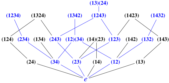
Figure 1. $\preceq$ on ${\mathcal{S}}_{4}$

Some of these structure constants $c^{w}_{u\,v(\lambda,k)}$ may be expressed in terms of chains in the Bruhat order. If $u\lessdot_{k}u(a,b)$ is a cover in the $k$-Bruhat order, label that edge of the Hasse diagram with the integer $u(b)$. The word of a chain in the $k$-Bruhat order is the sequence of labels of edges in the chain.

Theorem 3.3.

Suppose $u\leq_{k}w$ and $wu^{-1}$ is shape equivalent to $v(\mu,l)\cdot v(\nu,l)^{-1}$, for some $l$ and partitions $\mu\subset\nu$. Then, for any partition $\lambda$ and standard Young tableau $T$ of shape $\lambda$,

$$c^{w}_{u\,v(\lambda,k)}\ =\ \#\left\{\begin{array}[]{cc}\mbox{Chains in $k$-Bruhat order from $u$ to $w$ whose word}\\ \mbox{ has recording tableau $T$ under Schensted insertion}\end{array}\right\}.$$

Since a chain in the $k$-Bruhat order is a $\{k\}$-chain in the sense of §1, Theorem 3.3 gives a combinatorial proof of Theorem 1.1 when $wu^{-1}$ is shape equivalent to a skew partition. The key step is when $w$ and $u$ are Grassmannian permutations. In that case, symmetry of the Schensted algorithm reduces the theorem to showing the ‘diagonal word’ of a tableau is Knuth-equivalent to its reading word. By the diagonal word, we mean the entries of a tableau read first by their diagonal, and then in increasing order in each diagonal. For instance, this tableau has diagonal word $7\,58\,379\,148\,26\,26\,5\,8$.

There are many permutations $u,w$ which do not satisfy the hypotheses of Theorem 3.3, but for which the conclusion holds. For example, any $u,w$ for which $wu^{-1}=(143652)$ satisfy the conclusion, but $(143652)$ is not shape equivalent to any skew partition. However, some hypotheses are necessary. Let $u=312645$ and $w=561234$. Here is the labeled Hasse diagram of $[u,w]_{2}$:

There are six chains in this interval from which we obtain these recording tableaux:

  .

This list omits the tableau , and the third and fourth tableaux are identical.

We calculate $c^{w}_{u,v(\lambda,2)}$ using Theorem 5 of [22], or Theorem 4 (1) of [21]:

$$c^{w}_{u\;v(\begin{picture}(12.0,3.0)\put(0.0,0.0){\line(0,1){3.0}} \put(0.0,0.0){\line(1,0){12.0}} \put(3.0,0.0){\line(0,1){3.0}} \put(0.0,3.0){\line(1,0){12.0}} \put(6.0,0.0){\line(0,1){3.0}} \put(9.0,0.0){\line(0,1){3.0}} \put(12.0,0.0){\line(0,1){3.0}} \end{picture}\,,2)}\ =\ c^{w}_{u\;v(\,\begin{picture}(9.0,6.0)\put(0.0,0.0){\line(0,1){6.0}} \put(0.0,0.0){\line(1,0){9.0}} \put(3.0,0.0){\line(0,1){6.0}} \put(0.0,3.0){\line(1,0){9.0}} \put(6.0,0.0){\line(0,1){3.0}} \put(0.0,6.0){\line(1,0){3.0}} \put(9.0,0.0){\line(0,1){3.0}} \end{picture}\,,2)}\ =\ c^{w}_{u\;v(\,\begin{picture}(6.0,6.0)(0.0,0.0)\put(0.0,0.0){\line(0,1){6.0}} \put(0.0,0.0){\line(1,0){6.0}} \put(3.0,0.0){\line(0,1){6.0}} \put(0.0,3.0){\line(1,0){6.0}} \put(6.0,0.0){\line(0,1){6.0}} \put(0.0,6.0){\line(1,0){6.0}} \end{picture}\,,2)}\ =\ 1.$$

If a skew Young diagram $\kappa$ is the disjoint union of two incomparable diagrams $\rho$ and $\theta$, then

$$c^{\kappa}_{\lambda}\ =\ \sum_{\mu,\nu}c^{\lambda}_{\mu\,\nu}c^{\rho}_{\mu}c^{\theta}_{\nu}.$$

Similarly, we say that a product $\zeta\cdot\eta$ is disjoint if the two permutations $\zeta$ and $\eta$ have disjoint supports and $|\zeta\cdot\eta|=|\zeta|+|\eta|$. We have:

Theorem 3.4 (Disjointness).

Suppose $\zeta\cdot\eta$ is disjoint. Then

1. The map $(\alpha,\beta)\mapsto\alpha\cdot\beta$ induces an isomorphism $[e,\zeta]_{\preceq}\times[e,\eta]_{\preceq}\stackrel{{\scriptstyle\sim}}{{\longrightarrow}}[e,\zeta\cdot\eta]_{\preceq}$.

2. For all $\lambda$,  ${\displaystyle c^{\zeta\cdot\eta}_{\lambda}\ =\ \sum_{\mu,\nu}c^{\lambda}_{\mu\,\nu}c^{\zeta}_{\mu}c^{\eta}_{\nu}}$.

The next identity has no analogy with the classical Littlewood-Richardson coefficients. Let $(1\,2\,\ldots\,n)$ be the permutation which cyclicly permutes $[n]$.

Theorem 3.5 (Cyclic Shift).

Suppose $\zeta\in S_{n}$ and $\eta=\zeta^{(1\,2\,\ldots\,n)}$. Then, for any partition $\lambda$, $c^{\zeta}_{\lambda}=c^{\eta}_{\lambda}$.

This is proven using geometric arguments similar to those which establish Theorem 3.1 (ii). Combined with Theorem 1.1, we obtain:

Corollary 3.6.

If $u\leq_{k}w$ and $x\leq_{k}z$ with $wu^{-1},zx^{-1}\in{\mathcal{S}}_{n}$ and $(wu^{-1})^{(1\,2\,\ldots\,n)}=zx^{-1}$, then the two intervals $[u,w]_{k}$ and $[x,z]_{k}$ each have the same number of chains.

It would be interesting to give a bijective proof of Corollary 3.6. The two intervals $[u,w]_{k}$ and $[x,z]_{k}$ of Corollary 3.6 are typically non-isomorphic: In ${\mathcal{S}}_{4}$, let $u=1234$, $x=2134$, and $v=1324$. If $\zeta=(1243)$, $\eta=(1423)=\zeta^{(1234)}$, and $\xi=(1342)=\eta^{(1234)}$, then

$$u\ \leq_{2}\ \zeta u,\quad x\ \leq_{2}\ \eta x,\quad\mbox{and}\quad v\ \leq_{2}\ \xi v.$$

We illustrate the intervals $[u,\zeta u]_{2}$, $[x,\eta x]_{2}$, and $[v,\xi v]_{2}$.

4. Substitutions

The identities of §3 require a more general study of the behaviour of Schubert polynomials under certain specializations of the variables. This leads to a number of new formulas and identities.

For $w\in{\mathcal{S}}_{n+1}$ and $1\leq p\leq n+1$, let $w/_{p}\in{\mathcal{S}}_{n}$ be defined by deleting the $p$th row and $w(p)$th column from the permutation matrix of $w$. If $y\in{\mathcal{S}}_{n}$ and $1\leq q\leq n+1$, then $\varepsilon_{p,q}(y)\in{\mathcal{S}}_{n+1}$ is the permutation such that $\varepsilon_{p,q}(y)/_{p}=y$ and $\varepsilon_{p,q}(y)(p)=q$. The index of summation in a particular case of the Pieri-type formula [11, 22, 23],

$${\mathfrak{S}}_{v}\cdot(x_{1}\cdots x_{p-1})\quad=\quad\sum_{v\stackrel{{\scriptstyle c_{p}}}{{\relbar\joinrel\longrightarrow}}w}{\mathfrak{S}}_{w},$$

defines the relation $v\stackrel{{\scriptstyle c_{p}}}{{\relbar\joinrel\longrightarrow}}w$. More concretely, $v\stackrel{{\scriptstyle c_{p}}}{{\relbar\joinrel\longrightarrow}}w$ if and only if there is a chain in the $(p-1)$-Bruhat order:

$$v\ \lessdot_{p-1}\ (\alpha_{1},\beta_{1})v\ \lessdot_{p-1}\ \cdots\ \lessdot_{p-1}\ (\alpha_{p-1},\beta_{p-1})\cdots(\alpha_{1},\beta_{1})v\ =\ w$$

with $\beta_{1}>\beta_{2}>\cdots>\beta_{p-1}$.

Define $\Psi_{p}:{\mathbb{Z}}[x_{1},x_{2},\ldots]\rightarrow{\mathbb{Z}}[x_{1},x_{2},\ldots]$ by

$$\Psi_{p}(x_{j})\ =\ \left\{\begin{array}[]{ll}x_{j}&\mbox{ if }j<p\\ 0&\mbox{ if }j=p\\ x_{j-1}&\mbox{ if }j>p\end{array}\right..$$

Theorem 4.1.

Let $u,w\in{\mathcal{S}}_{\infty}$. Suppose $w(p)=u(p)$ and $\ell(w)-\ell(u)=\ell(w/_{p})-\ell(u/_{p})$, for some positive integer $p$. Then

1. $\varepsilon_{p,u(p)}:[u/_{p},w/_{p}]\stackrel{{\scriptstyle\sim}}{{\longrightarrow}}[u,w]$.

2. For any $v\in{\mathcal{S}}_{\infty}$,

   $$c^{w}_{u\,v}\quad=\quad\sum_{\stackrel{{\scriptstyle\mbox{\scriptsize$y\in{\mathcal{S}}_{\infty}$}}}{{v\stackrel{{\scriptstyle c_{p}}}{{\relbar\joinrel\longrightarrow}}\varepsilon_{p,1}(y)}}}c^{w/_{p}}_{u/_{p}\>y}.$$

3. For any $v\in{\mathcal{S}}_{\infty}$,

   $$\Psi_{p}({\mathfrak{S}}_{v})=\sum_{\stackrel{{\scriptstyle\mbox{\scriptsize$y\in{\mathcal{S}}_{\infty}$}}}{{v\stackrel{{\scriptstyle c_{p}}}{{\relbar\joinrel\longrightarrow}}\varepsilon_{p,1}(y)}}}{\mathfrak{S}}_{y}.$$

The first statement is proven using combinatorial arguments, while the second and third are proven by computing certain maps on cohomology. Since $c^{w}_{u\,v}=c^{w}_{v\,u}=c^{w_{0}u}_{v\>w_{0}w}$, Theorem 4.1 (ii) gives a recursion for $c^{w}_{u\,v}$ when one of $wu^{-1},wv^{-1}$, or $w_{0}uv^{-1}$ has a fixed point and the condition on lengths is satisfied.

Theorem 4.1 (iii) is both a generalization and a strengthening of the transition equations of [15]. We give an example: Let $v=413652$. Consider the part of the labeled Hasse diagram in the 2-Bruhat order above $v$ with decreasing edge labels. Then the leaves are those $w$ with $v\stackrel{{\scriptstyle c_{3}}}{{\longrightarrow}}w$.

Of these, only the two underlined permutations are of the form $\varepsilon_{3,1}(y)$:

$$631452\ =\ \varepsilon_{3,1}(52341)\quad\mbox{and}\quad 531642\ =\ \varepsilon_{3,1}(42531).$$

Thus Theorem 4.1 (iii) asserts that $\Psi_{3}({\mathfrak{S}}_{413652})={\mathfrak{S}}_{52341}+{\mathfrak{S}}_{42531}.$ Indeed,

$${\mathfrak{S}}_{413652} = x_{1}^{4}x_{2}x_{4}x_{5}+x_{1}^{3}x_{2}^{2}x_{4}x_{5}+x_{1}^{3}x_{2}x_{4}^{2}x_{5}+$$

$$x_{1}^{4}x_{2}x_{3}x_{4}+x_{1}^{4}x_{2}x_{3}x_{5}+x_{1}^{4}x_{3}x_{4}x_{5}+x_{1}^{3}x_{2}^{2}x_{3}x_{4}+x_{1}^{3}x_{2}^{2}x_{3}x_{5}+x_{1}^{3}x_{2}x_{3}^{2}x_{4}+$$

$$x_{1}^{3}x_{2}x_{3}^{2}x_{5}+x_{1}^{3}x_{2}x_{3}x_{4}^{2}+x_{1}^{3}x_{3}^{2}x_{4}x_{5}+x_{1}^{3}x_{3}x_{4}^{2}x_{5}+2\cdot x_{1}^{3}x_{2}x_{3}x_{4}x_{5},$$

so

$$\Psi_{3}({\mathfrak{S}}_{413652})=x_{1}^{4}x_{2}x_{3}x_{4}+x_{1}^{3}x_{2}^{2}x_{3}x_{4}+x_{1}^{3}x_{2}x_{3}^{2}x_{4}.$$

Since

$${\mathfrak{S}}_{52341}\ =\ x_{1}^{4}x_{2}x_{3}x_{4}\quad\mbox{ and}\quad{\mathfrak{S}}_{42531}\ =\ x_{1}^{3}x_{2}^{2}x_{3}x_{4}+x_{1}^{3}x_{2}x_{3}^{2}x_{4},$$

we see that

$$\Psi_{3}({\mathfrak{S}}_{413652})={\mathfrak{S}}_{52341}+{\mathfrak{S}}_{42531}.$$

We also compute the effect of other substitutions of the variables in terms of the Schubert basis: For $P\subset{\mathbb{N}}$, set $P^{c}:={\mathbb{N}}-P$ and list the elements of $P$ and $P^{c}$ in order:

$$P\ :\ p_{1}<p_{2}<\cdots\qquad\qquad P^{c}\ :\ p^{c}_{1}<p^{c}_{2}<\cdots$$

Define $\Psi_{P}:{\mathbb{Z}}[x_{1},x_{2},\ldots]\rightarrow{\mathbb{Z}}[y_{1},y_{2},\ldots,z_{1},z_{2},\ldots]$ by:

$$\Psi_{P}(x_{p_{j}})\ =\ y_{j}\qquad\mbox{and}\qquad\Psi_{P}(x_{p^{c}_{j}})\ =\ z_{j}.$$

Theorem 4.2.

Let $P\subset{\mathbb{N}}$ be as above. Then there exists an (explicitly described) infinite set $\Pi_{P}\subset{\mathcal{S}}_{\infty}$ such that for any $w\in{\mathcal{S}}_{n}$ and $\pi\in I_{P}-{\mathcal{S}}_{3n}$,

$$\Psi_{P}({\mathfrak{S}}_{w})\ =\ \sum_{u,\,v}c^{(u\times v)\cdot\pi}_{\pi\;w}\;{\mathfrak{S}}_{u}(y)\;{\mathfrak{S}}_{v}(z).$$

This generalizes [12, 1.5] (See also [18, 4.19]), where it is shown that the coefficients are nonnegative when $P=[n]$. Theorem 4.2 gives infinitely many identities of the form $c^{(u\times v)\cdot\pi}_{\pi\;w}=c^{(u\times v)\cdot\sigma}_{\sigma\;w}$ for $\pi,\sigma\in\Pi_{P}$. Moreover, for these $u,v$, and $\pi$, we have $[\pi,\;(u\times v)\cdot\pi]\simeq[e,u]\times[e,\,v]$, which is suggestive of a chain-theoretic basis for these identities.

5. Outline of geometric proofs

Many of these results are proven with arguments from geometry. Our main technique is as follows: If $u,w\in{\mathcal{S}}_{n}$, then

$$c^{w}_{u\,v(\lambda,k)}\ =\ \#\left(X_{w_{0}w}\bigcap X^{\prime}_{u}\bigcap X^{\prime\prime}_{v(\lambda,k)}\right),$$

where $X_{w_{0}w}$, $X^{\prime}_{u}$, and $X^{\prime\prime}_{v(\lambda,k)}$ are Schubert varieties in general position in the manifold ${\mathbb{F}}\ell_{n}$ of complete flags in ${\mathbb{C}}^{n}$. We reduce this to a computation in $\mbox{\em Grass}(k,n)$, the Grassmann manifold of $k$-planes in ${\mathbb{C}}^{n}$.

Let $\pi_{k}:{\mathbb{F}}\ell_{n}\rightarrow\mbox{\em Grass}(k,n)$ be the projection that sends a complete flag to its $k$-dimensional subspace. Since $X^{\prime\prime}_{v(\lambda,k)}=\pi_{k}^{-1}(\Omega^{\prime\prime}_{\lambda})$, where $\Omega^{\prime\prime}_{\lambda}$ is a Schubert subvariety of $\mbox{\em Grass}(k,n)$, we have

$$c^{w}_{u\,v(\lambda,k)}\ =\ \#\pi_{k}\left(X_{w_{0}w}\bigcap X^{\prime}_{u}\right)\bigcap\Omega^{\prime\prime}_{\lambda}.$$

Thus it suffices to study $\pi_{k}\left(X_{w_{0}w}\bigcap X^{\prime}_{u}\right)\subset\mbox{\em Grass}(k,n)$, equivalently, its fundamental cycle in homology, as

$$\left[\pi_{k}\left(X_{w_{0}w}\bigcap X^{\prime}_{u}\right)\right]\ =\ \sum_{\lambda}c^{w}_{u\,v(\lambda,k)}S_{\lambda^{c}},$$

where $S_{\lambda^{c}}$ is the homology class dual to the fundamental cycle of $\Omega^{\prime\prime}_{\lambda}$.

To prove Theorems 3.1 (ii) and Theorem 3.5, we first use Theorem 4.1 (ii) to reduce to the case of $k=l$ and $wu^{-1}=zx^{-1}$. Then we explicitly compute a dense subset of $X_{w_{0}w}\bigcap X^{\prime}_{u}$ and its image, $Y_{w,u}$, in $\mbox{\em Grass}(k,n)$. This analysis shows that, up to the action of the general linear group, $Y_{w,u}$ depends only upon $wu^{-1}$, up to conjugation by $(12\ldots n)$, whenever $wu^{-1}\in{\mathcal{S}}_{n}$.

For Theorem 4.2, we study maps

$$\Psi_{P}\ :\ {\mathbb{F}}\ell_{n}\times{\mathbb{F}}\ell_{m}\ \longrightarrow{\mathbb{F}}\ell_{n+m}$$

where $\Psi_{P}$ ‘shuffles’ pairs of flags together to obtain a longer flag, according to a set $P:1\leq p_{1}<\cdots<p_{n}\leq m$. We show that $\Psi_{P}(X_{u}\times X_{v})$ is an intersection of two Schubert varieties, which enables the computation of the map $(\Psi_{P})_{*}$ on homology. Then Poincaré duality determines the map $(\Psi_{P})^{*}$ on the Schubert basis of cohomology. By construction, $(\Psi_{P})^{*}$ acts by the substitution $\Psi_{P}$ of §4. In the case $m=1$, these computations become more precise, and we obtain Theorem 4.1 (i) and (ii).

Finally, for Theorem 3.4, suppose $\zeta\cdot\eta$ is disjoint and $u\leq_{k+l}(\zeta\cdot\eta)u$ with $u\in{\mathcal{S}}_{n+m}$. Then, set $P=u^{-1}{\rm supp}(\zeta)$ and consider the commutative diagram:

Here, $\varphi_{k,l}$ maps a pair $(H,K)\in\mbox{\it Grass}_{k}{\mathbb{C}}^{n}\times\mbox{\it Grass}_{l}{\mathbb{C}}^{m}$ to the sum $H\oplus K$ in $\mbox{\it Grass}_{k+l}{\mathbb{C}}^{n+m}$. We show there exists $x\in{\mathcal{S}}_{n}$, $y\in{\mathcal{S}}_{m}$ and $\zeta^{\prime},\eta^{\prime}$ shape-equivalent to $\zeta$ and $\eta$ such that $x\leq_{k}\zeta^{\prime}x$, $y\leq_{l}\eta^{\prime}y$, and

$$\Psi_{P}\left(X_{w_{0}\zeta^{\prime}x}\bigcap X^{\prime}_{x}\right)\times\left(X_{w_{0}\eta^{\prime}y}\bigcap X^{\prime}_{y}\right)\ =\ X_{w_{0}(\zeta\cdot\eta)u}\bigcap X^{\prime}_{u}.$$

Thus to compute $\pi_{k+l}(X_{w_{0}(\zeta\cdot\eta)u}\bigcap X^{\prime}_{u})$, or rather its homology class, it suffices to compute the map $(\varphi_{k,l})_{*}$ on homology, which is

$$(\varphi_{k,l})_{*}S_{\lambda}\ =\ \sum_{\mu,\nu}c^{\lambda}_{\mu\,\nu}S_{\mu}\otimes S_{\nu}.$$

For more details on these proofs and other aspects of this note, see [1].

References

• [1] N. Bergeron and F. Sottile, Schubert polynomials, the Bruhat order, and the geometry of flag manifolds. Duke Math. J., to appear.
• [2]  , A moniod for the universal $k$-Bruhat order. in preparation, 1997.
• [3] I. N. Bernstein, I. M. Gelfand, and S. I. Gelfand, Schubert cells and cohomology of the spaces $G/P$, Russian Mathematical Surveys, 28 (1973), pp. 1–26.
• [4] N. Bourbaki, Groupes et algèbres de Lie, Chap. IV, V, VI, 2ème édition, Masson, 1981.
• [5] I. Ciocan-Fontanine, On quantum cohomology of partial flag varieties. 1997.
• [6] M. Demazure, Désingularization des variétés de Schubert généralisées, Ann. Sc. E. N. S. (4), 7 (1974), pp. 53–88.
• [7] S. Fomin, S. Gelfand, and A. Postnikov, Quantum Schubert polynomials. J. AMS, to appear, 1997.
• [8] W. Fulton, Young Tableaux, with Applications to Representation Theory and Geometry, Cambridge University Press, 1996.
• [9] A. Kirillov and T. Maeno, Quantum Schubert polynomials and the Vafa-Intriligator formula, Tech. Rep. 96-41, University of Tokyo Mathematical Sciences, 1996.
• [10] A. Lascoux, Polynômes de Schubert: une approach historique, Discrete Math., 139 (1995), pp. 303–317.
• [11] A. Lascoux and M.-P. Schützenberger, Polynômes de Schubert, C. R. Acad. Sci. Paris, 294 (1982), pp. 447–450.
• [12]  , Structure de Hopf de l’anneau de cohomologie et de l’anneau de Grothendieck d’une variété de drapeaux, C. R. Acad. Sci. Paris, 295 (1982), pp. 629–633.
• [13]  , Symmetry and flag manifolds, in Invariant Theory, (Montecatini, 1982), vol. 996 of Lecture Notes in Math., Springer-Verlag, 1983, pp. 118–144.
• [14]  , Interpolation de Newton à plusieurs variables, in Sém. d’Algèbre M. P. Malliavin 1984-3, vol. 1146 of Lecture Notes in Math., Springer-Verlag, 1985, pp. 161–175.
• [15]  , Schubert polynomials and the Littlewood-Richardson rule, Lett. Math. Phys., 10 (1985), pp. 111–124.
• [16]  , Symmetrization operators on polynomial rings, Funkt. Anal., 21 (1987), pp. 77–78.
• [17] D. E. Littlewood and A. R. Richardson, Group characters and algebra, Philos. Trans. Roy. Soc. London., 233 (1934), pp. 99–141.
• [18] I. G. Macdonald, Notes on Schubert Polynomials, Laboratoire de combinatoire et d’informatique mathématique (LACIM), Université du Québec à Montréal, Montréal, 1991.
• [19] D. Monk, The geometry of flag manifolds, Proc. London Math. Soc., 9 (1959), pp. 253–286.
• [20] A. Postnikov, On a quantum version of pieri’s formula. Manuscript, 1997.
• [21] F. Sottile, A geometric approach to the combinatorics of Schubert polynomials, in Actes du 7éme Congress SFCA – 29 Mai - 2 Juin 1995., Mai 1995. Edité par B. Leclerc et J.Y. Thibon, pp 501–511. Extended abstract of talk.
• [22]  , Pieri’s formula for flag manifolds and Schubert polynomials, Annales de l’Institut Fourier, 46 (1996), pp. 89–110.
• [23] R. Winkel, On the multiplication of Schubert polynomials. manuscript, http://www-math.mit.edu/$\tilde{\ }$winkel, 1996.