McKay correspondence

1 Introduction

Conjecture 1.1 (since 1992)

$G\subset\operatorname{SL}(n,{\mathbb{C}})$ is a finite subgroup. Assume that the quotient $X={\mathbb{C}}^{n}/G$ has a crepant resolution $f\colon Y\to X$ (this just means that $K_{Y}=0$, so that $Y$ is a “noncompact Calabi–Yau manifold”). Then there exist “natural” bijections

$$\{\text{\em irreducible representations of $G$}\} \to\text{\em basis of $H^{*}(Y,{\mathbb{Z}})$}$$ (1)

$$\{\text{\em conjugacy classes of $G$}\} \to\text{\em basis of $H_{*}(Y,{\mathbb{Z}})$}$$ (2)

As a slogan “$\text{representation theory of $G$}=\text{homology theory of $Y$}$”.

Moreover, these bijections satisfy “certain compatibilities”

$$\left.\begin{array}[]{rr}\text{\em character table of $G$}\\ \text{\em McKay quiver}\end{array}\right\}\leftrightarrow\left\{\begin{array}[]{ll}\text{\em duality}\\ \text{\em cup product}\end{array}\right.$$

As you can see, the statement is still too vague because I don’t say what “natural” means, and what “compatibilities” to expect. At present it seems most useful to think of this statement as pointer towards the truth, rather than the truth itself (compare Main Conjecture 4.1).

The conjecture is known for $n=2$ (Kleinian quotient singularities, Du Val singularities). McKay’s original treatment was mainly combinatorics [McK]. The other important proof is that of Gonzales-Sprinberg and Verdier [GSp-V], who introduced the GSp–V or tautological sheaves, also my main hope for the correspondence (1).

For $n=3$ a weak version of the correspondence (2) is proved in [IR]. We hope that a modification of this idea will work in general for (2); for details, see §3.

Contents

This is a rough write-up of my lecture at Kinosaki and two lectures at RIMS workshops in Dec 1996, on work in progress that has not yet reached any really worthwhile conclusion, but contains lots of fun calculations. History of Vafa’s formula, how McKay correspondence relates to mirror symmetry. The main aim is to give numerical examples of how the McKay correspondences (1) and (2) must work, and to restate Conjecture 1.1 as a tautology, like the cohomology or K-theory of projective space ${\mathbb{P}}^{n}$ (see Main Conjecture 4.1). Introduction to Nakamura’s results on the Hilbert scheme of $G$-clusters.

Credits

Very recent results of I. Nakamura on $G$-Hilb, who sent me a first draft of [N3] and many helpful explanations. Joint work with Y. Ito. Moral support and invaluable suggestions of S. Mukai. Support Sep–Nov 1996 by the British Council–Japanese Ministry of Education exchange scheme, and from Dec 1996 by Nagoya Univ., Graduate School of Polymathematics.

1.1 History

Around 1986 Vafa and others defined the stringy Euler number for a finite group $G$ acting on a manifold $M$:

$$e_{\text{string}}(M,G) =\text{crazy formula (you'd better forget it!)} *$$ ()

$$=\sum_{H\subset G}e(X_{H})\times\operatorname{\#}\{\text{conjugacy classes in $H$}\}.$$

Here $X=M/G$, and $X$ is stratified by stabiliser subgroups: for a subgroup $H\subset G$, set

$$M_{H} =\{Q\in M|\operatorname{Stab}_{G}Q=H\},$$

$$X_{H} =\pi(M_{H})$$

$$=\{P\in X|\text{for $Q\in\pi^{-1}(P)$, $\operatorname{Stab}_{G}Q$ is conjugate to $H$}\}.$$

The sum in ($*$) runs over all subgroups $H$, and $e(X_{H})$ is the ordinary Euler number. The mathematical formulation ($*$) is due to Hirzebruch–Höfer [HH] and Roan [Roan]. If $M={\mathbb{C}}^{n}$ and $G\subset\operatorname{GL}(n,{\mathbb{C}})$ only fixes the origin, then the closure of each $X_{H}$ is contractible, so that only the origin $\{0\}=X_{G}$ contributes to the sum in ($*$), and

$$e_{\text{string}}({\mathbb{C}}^{n},G)=\operatorname{\#}\{\text{conjugacy classes in $G$}\}.$$

At the same time, Vafa and others conjectured the following:

Conjecture 1.2 (“physicists’ Euler number conjecture”)

In appropriate circumstances,

$$e_{\text{\em string}}(M,G)=\text{\em Euler number of minimal resolution of $M/G$.}$$

The context is string theory of $M=\text{CY 3-fold}$, and the $G$ action on $M$ is Gorenstein, meaning that it fixes a global basis $s\in\omega_{M}={\cal O}(K_{M})\cong{\cal O}_{M}$ (dualising sheaf $\omega_{M}=\Omega^{3}_{M}$). In particular, for any point $Q\in M$, the stabiliser subgroup is in $\operatorname{SL}(T_{Q}M)$.

At that time, the physicists possibly didn’t know that there was a generation of algebraic geometers working on minimal models of 3-folds, and possibly naively assumed that in their cases, there exists a unique minimal resolution $Y\to X=M/G$, so that $e_{\text{string}}(M,G)=e(Y)$. A number of smart-alec 3-folders raised various instinctive objections, that a minimal model may not exist, is usually not unique etc.

However, it turns out that the physicists were actually nearer the mark. One of the points of these lectures is that, in flat contradiction to the official 3-fold ideology of the last 15 years, in many cases of interest, there is a distinguished crepant resolution, namely Nakamura’s $G$-Hilbert scheme.

My guess of the McKay correspondences follow on naturally from Vafa’s conjecture, by the following logic. If $M={\mathbb{C}}^{n}$, then one sees easily that for any reasonable resolution of singularities $Y\to X={\mathbb{C}}^{n}/G$, the cohomology is spanned by algebraic cycles, so that

$$e(Y)=\sum H^{p,p}=\operatorname{\#}\{\text{algebraic cycles of $Y$}\}.$$

It seems unlikely that we could prove the numerical concidence

$$e(Y)=\operatorname{\#}\{\text{conjugacy classes of $G$}\}$$

without setting up some kind of bijection between the two sets. [IR] does so for $G\subset\operatorname{SL}(3,{\mathbb{C}})$.

1.2 Relation with mirror symmetry, applications

Consider:

1. the search for mirror pairs;

2. Vafa’s conjecture;

3. conjectural McKay correspondence;

4. speculative theory of equivariant mirror symmetry ($G$-mirror symmetry).

Historically, (a) led to (b), (b) led to (c), and logically (c) implies (b). I have long speculated that (c) is connected to (d), and maybe even that it would eventually be proved in terms of (d). The point is that up to now, the known proofs of the McKay correspondence (even in 2 dimensions) rely on the explicit classification of the groups, plus quite detailed calculations, and it would be very interesting to get more direct relations.

I suggest below in §4 that the McKay correspondence can be derived in tautological terms. If this works, it will have applications to (d). Some trivial aspects of this are already contained in Candelas and others’ example of the mirror of the quintic 3-fold [C], where you could take intermediate quotients in the $({\mathbb{Z}}/5)^{3}$ Galois tower. My suggestion is that $G$-mirror symmetry should relate pairs of CYs with group actions, and include the character theory of finite groups as the zero dimensional case. I guess you’re supposed to add an analog of “complexified Kähler parameters” to the conjugacy classes, and “complex moduli” to the irreducible representations. Another application (more speculative, this one) might be to wake up a few algebraists.

1.3 Conjecture 1.1, (1) or (2), which is better?

I initially proposed Conjecture 1.1 in 1992 in terms of irreducible representations, an analog of the formulations of McKay and of [GSp-V]. I was persuaded by social pressure around the Trento conference and by my coauthor Yukari Ito to switch to (2); its advantage is that the two sides are naturally graded, and we could prove a theorem [IR]. Batyrev and Kontsevich and others have argued more recently that (2) is the more fundamental statement. However, the version of correspondence (2) in cohomology stated in [IR] gives a ${\mathbb{Q}}$-basis only: the crepant divisors do not base $H^{2}(Y,{\mathbb{Z}})$ in general: fractional combinations of them turn up as $c_{1}({\cal L})$ for line bundles on $Y$ that are eigensheaves of the group action, that is, GSp-V sheaves for 1-dimensional representations of $G$.

These lectures return to (1), passing via K-theory; in this context, the natural structure on the right hand side of (1) is not the grading of $H^{*}$, but the filtration of $K_{0}Y$. In fact, my thoughts on (2) in general are, to be honest, in a bit of a mess at present (see §3 and §6 below).

2 First examples

These preliminary examples illustrate the following points:

1. To construct a resolution of a quotient singularity ${\mathbb{C}}^{n}/G$, and a very ample linear system on it, rather than invariant rational functions, it is more efficient to use ratios of covariants, that is, ratios of functions in the same character space. This leads directly to the Hilbert scheme as a natural candidate for a resolution.

2. Functions in a given character space $\rho$ define a tautological sheaf ${\cal F}_{\rho}$ on the resolution $Y\to X$, and in simple examples, you easily cook up combinations of Chern classes of the ${\cal F}_{\rho}$ to base the cohomology of $Y$.

I fix the following notation: $G\subset\operatorname{GL}(n,{\mathbb{C}})$ is a finite subgroup, $X={\mathbb{C}}^{n}/G$ the quotient, and $Y\to X$ a crepant resolution (if it exists). For a given cyclic (or Abelian) group, I choose eigencoordinates $x_{1},\dots,x_{n}$ or $x,y,z,\dots$ on ${\mathbb{C}}^{n}$. I write $\frac{1}{r}(a_{1},\dots,a_{n})$ for the cyclic group ${\mathbb{Z}}/r$ action given by $x_{i}\mapsto\varepsilon^{a_{i}}x_{i}$, where $\varepsilon=\exp(2\pi i/r)=\text{fixed primitive $r$th root of 1}$. Other notation, for example the lattice $L={\mathbb{Z}}^{n}+{\mathbb{Z}}\cdot\frac{1}{r}(a_{1},\dots,a_{n})$ of weights, and the junior simplex $\Delta_{\text{junior}}\subset L_{\mathbb{R}}$ are as in [IR].

Example 2.1

The

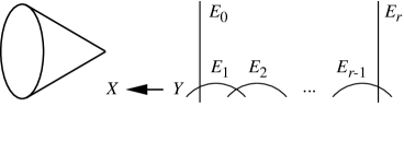
Figure 1: $E_{0}$ and $E_{r}$ are the image of the $x$ and $y$ axes

quotient singularity $\frac{1}{r}(1,-1)$. The notation means the cyclic group $G={\mathbb{Z}}/r$ acting on ${\mathbb{C}}^{2}$ by $(x,y)\mapsto(\varepsilon x,\varepsilon^{r-1}y)$. Everyone knows the invariant monomials $u=x^{r},v=xy,w=y^{r}$, the quotient map

$${\mathbb{C}}^{2}\to X={\mathbb{C}}^{2}/G=\text{Du Val singularity $A_{r-1}$}:(uw=v^{r})\subset{\mathbb{C}}^{3},$$

and the successive blowups that give the resolution $Y\to X$ and its chain of $-2$-curves $E_{1},\dots,E_{r-1}$ (Figure 1). However, the new point to note is that each $E_{i}$ is naturally parametrised by the ratio $x^{i}:y^{r-i}$. More precisely, an affine piece $Y_{i}\subset Y$ of the resolution is given by ${\mathbb{C}}^{2}$ with parameters $\lambda,\mu$, and the equations

$$x^{i}=\lambda y^{r-i},\quad y^{r-i+1}=\mu x^{i-1}\quad\text{and}\quad xy=\lambda\mu$$ (3)

define the $G$-invariant rational map ${\mathbb{C}}^{2}\mathrel{{\relbar\kern-0.2pt\rightarrow}}Y_{i}$ (quotient map and resolution at one go).

The ratio $x^{i}:y^{r-i}$ defines a linear system $|L(i)|$ on $Y$, with intersection numbers

$$L(i)\cdot E_{j}=\delta_{ij}\quad\text{(Kronecker $\delta$).}$$

Thus, writing ${\cal L}(i)$ for the corresponding sheaf or line bundle gives a natural one-to-one correspondence from nontrivial characters of $G$ to line bundles on $Y$ whose first Chern classes $c_{1}({\cal L}(i))\in H^{2}(Y,{\mathbb{Z}})$ give the dual basis to the natural basis $[E_{i}]$ of $H_{2}(Y,{\mathbb{Z}})$.

Example 2.2

One way of generalising Example 2.1 to dimension 3. Let

$$G=\left<\frac{1}{r}(1,-1,0),\frac{1}{r}(0,1,-1),\frac{1}{r}(-1,0,1,)\right>=({\mathbb{Z}}/r)^{2}\subset\operatorname{SL}(3,{\mathbb{C}})$$

be the maximal diagonal Abelian group of exponent $r$. Then the first quadrant of $L_{\mathbb{R}}$ has an obvious triangulation

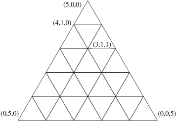
Figure 2: Triangulation of $\Delta_{\text{junior}}$ in Example 2.2

by regular simplicial cones that are basic for $L$ and have vertexes in the junior simplex $\Delta_{\text{junior}}$. By toric geometry and the standard discrepancy calculation [YPG], this triangulation defines a crepant resolution $Y\to X={\mathbb{C}}^{3}/G$.

From now on, restrict for simplicity to the case $r=5$ (featured on the mirror of the quintic [C]), whose triangulation is illustrated in Figure 2. $X={\mathbb{C}}^{3}/G$ has lines of Du Val singularities $A_{4}=\frac{1}{5}(1,-1)$ along the 3 coordinate axes, the fixed locuses of the 3 generating subgroups $\frac{1}{5}(1,-1,0)$ etc., of $G$.

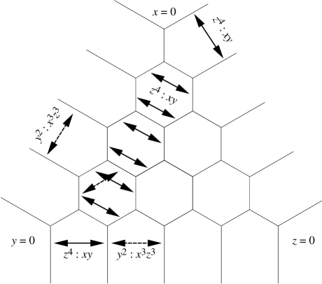
Figure 3: The resolution corresponding to the triangulation of Figure 2

As illustrated in Figure 3, the resolution $Y$ has 3 chains of 4 ruled surfaces over the coordinate axes of $X$, and 6 del Pezzo surfaces of degree 6 (“regular hexagons”) over the origin. Every exceptional curve stratum in the resolution is a $(-1,-1)$ curve.

Functions on the quotient $X={\mathbb{C}}^{3}/G$ are given by $G$-invariant polynomials, $k[X]={\mathbb{C}}[x,y,z]^{G}$. To get more functions on $Y$ (and a projective embedding of $Y$), consider the following ratios of monomials in the same eigenspace of the $G$ action:

$$x^{i}:(yz)^{5-i}\quad\text{for $i=1,\dots,4$, and permutations of $x,y,z$.}$$ (4)

Each ratio (4) defines a free linear system on $Y$, and all together, they define a relative embedding of $Y$ into a product of many copies of ${\mathbb{P}}^{1}$.

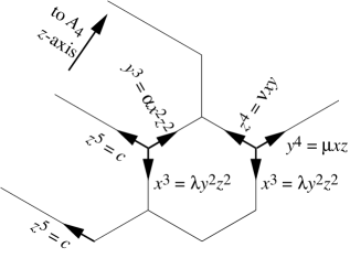
Figure 4: Two affine pieces near the hexagon at (3,1,1)

For example, as shown in Figure 4, the toric stratum at $(2,2,1)$ is a del Pezzo surface of degree 6 embedded by the 3 ratios $x^{3}:y^{2}z^{2}$, $y^{3}:x^{2}z^{2}$ and $z^{4}:xy$ (having product the trivial ratio $1:1$). Figure 4 shows two affine pieces of $Y$, of which the right-hand one is ${\mathbb{C}}^{3}$ with coordinates $\lambda,\mu,\nu$ related to $x,y,z$ by a set of equations generalising (3):

$$\begin{matrix}x^{3}&=&\lambda y^{2}z^{2}\\ y^{4}&=&\mu xz\\ z^{4}&=&\nu xy\end{matrix}\qquad\begin{matrix}y^{3}z^{3}&=&\mu\nu x^{2}\\ x^{2}z^{2}&=&\lambda\nu y^{3}\\ x^{2}y^{2}&=&\lambda\mu z^{3}\end{matrix}\quad\text{and}\quad xyz=\lambda\mu\nu.$$ (5)

Denote the linear system $|x^{i}:(yz)^{5-i}|$ by $|L(x^{i})|$, and similarly for permutations of $x,y,z$. The sum of all the $|L(x^{i})|$ is very ample on $Y$, but their first Chern classes do not span $H^{2}(Y,{\mathbb{Z}})$. To see this, recall the del Pezzo surface $S_{6}$ of degree 6, the 3 point blowup of ${\mathbb{P}}^{2}$ familiar from Cremona and Max Noether’s elementary quadratic transformation. It has 3 maps to ${\mathbb{P}}^{1}$ and 2 maps to ${\mathbb{P}}^{2}$; write $e_{1},e_{2},e_{3}$ for the divisor classes of the maps to ${\mathbb{P}}^{1}$, and $f_{1},f_{2}$ for the maps to ${\mathbb{P}}^{2}$. Then clearly,

$$\begin{gathered}e_{1},e_{2},e_{3},f_{1},f_{2}\quad\text{span}\quad H^{2}(S_{6},{\mathbb{Z}}),\\ \text{with the single relation}\quad e_{1}+e_{2}+e_{3}=f_{1}+f_{2}.\end{gathered}$$ (6)

For $S_{6}$ one of the hexagons of Figure 3, the 3 maps to ${\mathbb{P}}^{1}$ are provided by certain of the linear systems $|L(x^{i})|$. The two maps to ${\mathbb{P}}^{2}$ are provided by other character spaces: for example, for the $(2,2,1)$ hexagon of Figure 4, $f_{1}$ and $f_{2}$ are given by the linear systems $|L(x^{3}y)|$ and $|L(xy^{3})|$ corresponding respectively to the ratios

$$\left(x^{2}z^{4}:x^{3}y:y^{3}z^{2}\right)\quad\text{and}\quad\left(xy^{3}:y^{2}z^{4}:x^{3}z^{2}\right)=\left({1\over x^{2}z^{4}}:{1\over x^{3}y}:{1\over y^{3}z^{2}}\right).$$

For each surface $S_{6}$, the generators $e_{1},e_{2},e_{3},f_{1},f_{2}$ correspond to certain characters of $G$. For example, if I choose the 3 generators $\frac{1}{5}(1,-1,0)$, $\frac{1}{5}(0,1,-1)$ and $\frac{1}{5}(-1,0,1)$ of $G$, the characters of $x,y,z$ are

$$\begin{array}[]{rrr}x&y&z\\ \hline\cr 1&-1&0\\ 0&1&-1\\ -1&0&1\end{array}\quad\text{and my $(2,2,1)$ hexagon has}\quad\begin{array}[]{ccc|cc}e_{1}&e_{2}&e_{3}&f_{1}&f_{2}\\ x^{3}&y^{3}&z^{4}&x^{3}y&xy^{3}\\ \hline\cr 3&2&0&2&3\\ 0&3&1&1&3\\ 2&0&4&2&4\end{array}$$

Moreover, you see easily that the relations (6) actually hold in $H^{2}(Y,{\mathbb{Z}})$, not just in $H^{2}(S_{6},{\mathbb{Z}})$.

Represent each character of $G$ by a monomial $x^{m}$ (such as $x^{i}$ or $x^{3}y$); this corresponds to a free linear system $|L(x^{m})|$ on $Y$, in much the same way as the $L(x^{i}:(yz)^{r-i})$ or $L(x^{2}z^{4}:x^{3}y:y^{3}z^{2})$ just described.

Now the McKay correspondence (1) of Conjecture 1.1 is the following recipe:

$$\text{monomial $x^{m}$}\mapsto\text{line bundle ${\cal L}(x^{m})$}\mapsto c_{1}({\cal L}(x^{m}))\in H^{2}(Y,{\mathbb{Z}}).$$

These elements generate $H^{2}(Y,{\mathbb{Z}})$, with one relation of the form (6) for every regular hexagon $S_{6}$ of the picture. Moreover, each relation (6) gives an element

$$c_{2}(L(e_{1})\oplus L(e_{2})\oplus L(e_{3}))-c_{2}(L(f_{1})\oplus L(f_{2}))\in H^{4}(Y,{\mathbb{Z}}),$$ (7)

which is the dual element to $[S_{6}]\in H_{4}(Y,{\mathbb{Z}})$. Indeed,

$$c_{2}(L(e_{1})\oplus L(e_{2})\oplus L(e_{3}))\cdot S_{6} =e_{1}e_{2}+e_{1}e_{3}+e_{2}e_{3}=3,$$

$$\text{and}\quad c_{2}(L(f_{1})\oplus L(f_{2}))\cdot S_{6} =f_{1}f_{2}=2.$$

I draw the McKay correspondence resulting from this cookery in Figure 5: each edge $E\cong{\mathbb{P}}^{1}$ is labelled by the linear system $L(x^{m})$ with $L(x^{m})\cdot E=1$, and each hexagon $S_{6}$ by 2 characters corresponding to the two extra generators $f_{1},f_{2}$ of $H^{2}(S_{6},{\mathbb{Z}})$ with the relation which gives the dual element of $H^{4}(Y,{\mathbb{Z}})$.

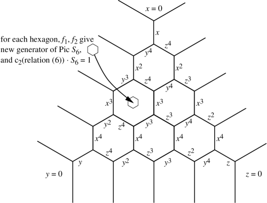
Figure 5: McKay correspondence for Example 2.2

One of the morals of this example is that we get a basis of cohomology in terms of Chern classes of virtual sums of tautological bundles; this suggests using the tautological bundles to base the K-theory of $Y$, and passing from K-theory to cohomology by Chern classes or Chern characters. In fact, the combinations used in (7) were fixed up to have zero first Chern class, exactly what you must do if you want the second Chern character to come out an integral class.

3 Ito–Reid, and the direct correspondence (2)

A group $G\subset\operatorname{SL}(n,{\mathbb{C}})$ has a natural filtration by age. Namely, any element $g\in G$ can be put in diagonal form by choosing $x_{1},\dots,x_{n}$ to be eigencoordinates of $g$. We write $g=\frac{1}{r}(a_{1},\dots,a_{n})$ to mean that

$$g:(x_{1},x_{2},\dots,x_{n})\mapsto(\varepsilon^{a_{1}}x_{1},\varepsilon^{a_{2}}x_{2},\dots,\varepsilon^{a_{n}}x_{n}),$$

where $\varepsilon=\exp(2\pi i/r)=\text{fixed primitive $r$th root of 1}$, and $a_{i}\in[0,1,\dots,n-1]$. Toric geometry tells us to consider the lattice

$$L={\mathbb{Z}}^{n}+{\mathbb{Z}}\frac{1}{r}(a_{1},\dots,a_{n})$$

(more generally for $A\subset G$ an Abelian group, we would add in lots of vectors $\frac{1}{r}(a_{1},\dots,a_{n})$ for each $g\in A$). This consists of weightings on the $x_{i}$, so that the invariant monomials have integral weights. Then for any element $b=\frac{1}{r}(b_{1},\dots,b_{n})\in L$ with all $b_{i}\geq 0$ (that is, $b$ in the positive quadrant), define

$$\operatorname{age}(b)=\frac{1}{r}\sum b_{i}.$$

In particular, for $g=\frac{1}{r}(a_{1},\dots,a_{n})$ in the unit cube,

$$\operatorname{age}(g)=\frac{1}{r}\sum a_{i};$$

this is obviously an integer (because $g\in\operatorname{SL}(n,{\mathbb{C}}))$ in the range $[0,n-1)$, and this defines the age filtration.

Now any primitive vector $b=\frac{1}{r}(b_{1},\dots,b_{n})\in L$ and in the positive quadrant defines a monomial valuation $v_{b}$ on the function field $k(X)$ of $X$. Furthermore, the standard discrepancy calculation (see [YPG]) says that

$$\operatorname{disc}(v_{b})=\operatorname{age}(b)-1.$$

Reminder:

The discrepancy $\operatorname{disc}v_{b}$ means that if I make a blowup $W_{b}\to X$ so that $v_{b}$ is the valuation at a prime divisor $F_{b}\subset W_{b}$, then $K_{W_{b}}=K_{X}+\operatorname{disc}(v_{b})F_{b}$. Note also that junior means $\operatorname{age}=1$, and crepant means $\text{discrepancy}=0$. Any other questions?

The valuation $b$ defines a locus $E_{b}=\operatorname{centre}(v_{b})\subset Y$. Consider only weightings $b$ such that $v_{b}$ is the valuation of $E_{b}\subset Y$; this means that if I blow up $Y$ along $E_{b}$, and $F_{b}$ is the exceptional divisor, then $v_{b}$ is the valuation associated with the prime divisor $F_{b}\subset\widetilde{Y}$. Since $Y$ is crepant, the adjunction formula for a blowup gives

$$\operatorname{disc}(v_{b})=\operatorname{codim}E_{b}-1,\quad\text{that is,}\quad\operatorname{codim}E_{b}=\operatorname{age}(b).$$

In [IR], we uses this idea to give a bijection

$$\{\text{junior conjugacy classes of $G$}\}\to\{\text{crepant valuations of $X$}\}$$

which gave us a basis of $H^{2}(Y,{\mathbb{Q}})$, and we dealt with $H^{4}(Y,{\mathbb{Q}})$ by Poincaré duality. Thus [IR] only used the valuation theoretic construction

$$b\mapsto v_{b}\mapsto E_{b}$$

for $b$ in the junior simplex $\Delta_{\text{junior}}$. However, the same idea obviously extends to give a correspondence from certain “good” elements $b$ to a set of locuses in $Y$ which generate $H_{*}(Y,{\mathbb{Z}})$. Thus the idea for the direct correspondence (2) is

$$G\ni g \mapsto\text{collection of suitable $b$}$$

$$\mapsto\text{collection of locuses $E_{b}\subset Y$}.$$

The first step is by a mysterious cookery, which I only indicate by the labelling in the two examples of §6 below (it should be possible to extract a good conjectural statement from this data).

4 Tautological sheaves and the main conjecture

These lectures are mainly concerned with providing experimental data for a suitably rephrased Conjecture 1.1, (1). In this section, I speculate on a framework to explain what is going on, that might eventually lead to a proof.

The following is the main idea of [GSp-V]. Given $G\subset\operatorname{SL}(n,{\mathbb{C}})$, we choose once and for all a complete set of irreducible representations $\rho\colon G\to\operatorname{GL}(V_{\rho})$. I use $\pi_{*}$ to view sheaves on ${\mathbb{C}}^{n}$ such as the structure sheaf ${\cal O}_{{\mathbb{C}}^{n}}$ as sheaves on the quotient $\pi\colon{\mathbb{C}}^{n}\to X$. Since $X$ is affine, these are really simply modules over $k[X]=k[{\mathbb{C}}^{n}]^{G}$, so I usually omit $\pi_{*}$. Note that $k({\mathbb{C}}^{n})$ is a Galois extension of $k(X)$, so that, by the cyclic element theorem of Galois theory, it is the regular representation of $G$, that is, $k({\mathbb{C}}^{n})=k(X)[G]$; thus $\pi_{*}{\cal O}_{{\mathbb{C}}^{n}}$ is generically isomorphic to the regular representation ${\cal O}_{X}[G]$. For each $\rho$, set

$${\cal F}^{\prime}_{\rho}:=\operatorname{Hom}(V_{\rho},{\cal O}_{{\mathbb{C}}^{n}})^{G}$$

Then ${\cal F}^{\prime}_{\rho}\otimes V_{\rho}\subset{\cal O}_{{\mathbb{C}}^{n}}$ is the character subsheaf corresponding to $V_{\rho}$; by the usual decomposition of the regular representation, ${\cal F}^{\prime}_{\rho}$ is a sheaf of ${\cal O}_{X}$-modules of rank $\deg\rho$. And there is a canonical decomposition

$${\cal O}_{{\mathbb{C}}^{n}}=\sum_{\rho}{\cal F}^{\prime}_{\rho}\otimes V_{\rho}\quad\text{as ${\cal O}_{X}[G]$ modules.}$$

Now let $f\colon Y\to X$ be a given resolution. Each ${\cal F}^{\prime}_{\rho}$ has a birational transform ${\cal F}_{\rho}$ on $Y$. This means that ${\cal F}_{\rho}$ is the torsion free sheaf of ${\cal O}_{Y}$ modules generated by ${\cal F}^{\prime}_{\rho}$, or if you prefer, ${\cal F}_{\rho}=f^{*}{\cal F}^{\prime}_{\rho}/(\text{torsion})$.

The sheaves ${\cal F}_{\rho}$ are the GSp-V sheaves, or the tautological sheaves of $Y$. Note that by definition, the ${\cal F}_{\rho}$ are generated by their $H^{0}$.

Conjecture 4.1 (Main conjecture)

Under appropriate circumstances, thetautological sheaves ${\cal F}_{\rho}$ form a ${\mathbb{Z}}$-basis of the Grothendieck group $K_{0}(\operatorname{Coh}Y)$, and a certain cookery with their Chern classes leads to a ${\mathbb{Z}}$-basis of $H^{*}(Y,{\mathbb{Z}})$. A slightly stronger conjecture is that the ${\cal F}_{\rho}$ form a ${\mathbb{Z}}$-basis of the derived category $D^{b}(\operatorname{Coh}Y)$.

Remark 4.2

“Appropriate circumstances” in the conjecture include all cases when $G\subset\operatorname{SL}(n,{\mathbb{C}})$ and $Y=\operatorname{{\mbox{$G$}}-Hilb}$ is a crepant resolution. In this case, these tautological sheaves ${\cal F}_{\rho}$ have lots of good properties (see §5). But flops should not make too much difference to the statement – one expects a flopped variety $Y^{\prime}$ to have more or less the same homology and cohomology as $Y$, at least additively.

Example 4.3

$\frac{1}{n}(1,\dots,1)$ (with $n$ factors). The quotient $X$ is the cone on the $n$th Veronese embedding of ${\mathbb{P}}^{n-1}$, and the resolution $Y$ is the anticanonical bundle of ${\mathbb{P}}^{n-1}$, containing the exceptional divisor ${\mathbb{P}}^{n-1}$ with normal bundle ${\cal O}(-n)=\omega_{{\mathbb{P}}^{n}}$. The tautological sheaves are

$${\cal O},{\cal O}(1),\dots,{\cal O}(n-1).$$

That is, these are sheaves on $Y$ restricting down to the first $n$ multiples of ${\cal O}(1)$ on ${\mathbb{P}}^{n-1}$. It is well known that these sheaves form a ${\mathbb{Z}}$-basis of the Grothendieck group $K_{0}({\mathbb{P}}^{n-1})$. It is a standard (not quite trivial) bit of cookery with Chern classes and Chern characters to go from this to a ${\mathbb{Z}}$-basis of $H^{*}({\mathbb{P}}^{n-1},{\mathbb{Z}})$.

Remark 4.4

Recall the original (1977) Beilinson diagonal trick: the diagonal $\Delta_{{\mathbb{P}}^{n-1}}\subset{\mathbb{P}}^{n-1}\times{\mathbb{P}}^{n-1}$ is defined by the section

$$s_{\Delta}=\sum x_{i}^{\prime}{\partial\ \over\partial x_{i}}\in p_{1}^{*}{\cal O}_{{\mathbb{P}}^{n-1}}(1)\otimes p_{2}^{*}T_{{\mathbb{P}}^{n-1}}(-1).$$

Therefore, it follows (tautologically) that the derived category $D^{b}(\operatorname{Coh}{\mathbb{P}}^{n-1})$ (hence also the K theory $K_{0}$) has two “dual” bases

$${\cal O},\Omega^{1}(1),\dots,\Omega^{n-1}(n-1)\quad\text{vs.}\quad{\cal O},{\cal O}(-1),\dots,{\cal O}(-(n-1)).$$

Lame attempt to prove Conjecture 4.1

Step I

The resolution $Y\to X$ is the quotient $A/H$ of an open set $A\subset{\mathbb{C}}^{N}$ by a connected algebraic group $H$. In other words, by adding extra variables in a suitable way, we can arrange to make the finite quotient $X={\mathbb{C}}^{n}/G$ equal to the quotient ${\mathbb{C}}^{N}/H$ of a bigger space by the action of a connected group $H$ (the quotient singularities arise from jumps in the stabiliser group of the $H$-action); moreover, we can arrange to obtain the resolution $Y\to X$ by first deleting a set of “unstable” points of ${\mathbb{C}}^{N}$ and then taking the new quotient $A/H$. For example, the Veronese cone singularity of Example 4.3 is ${\mathbb{C}}^{n+1}$ divided by

$${\mathbb{C}}^{*}\ni\lambda\colon(x_{1},\dots,x_{n};z)\mapsto(\lambda x_{1},\dots,\lambda x_{n};\lambda^{-n}z).$$

(Obvious if you think about the ring of invariants). The finite group ${\mathbb{Z}}/n$ is the stabiliser group of a point of the $z$-axis. The blowup is the quotient $A/{\mathbb{C}}^{*}$, where $A={\mathbb{C}}^{n+1}\setminus\text{$z$-axis}$. (Because at every point of $A$, at least one of the $x_{i}\neq 0$, so the invariant ratios $x_{j}/x_{i}$ are defined locally as functions on the quotient.)

Step II

Most optimistic form: the Beilinson diagonal trick may apply to a quotient of the form obtained in Step I. That is, the diagonal $\Delta_{Y}\subset Y\times Y$ has ideal sheaf ${\cal I}_{\Delta_{Y}}$ resolved by an exact sequence in which all the other sheaves are of the form ${\cal F}_{i}\boxtimes{\cal G}_{i}=p_{1}^{*}{\cal F}_{i}\otimes p_{2}^{*}{\cal G}_{i}$, where the ${\cal F}_{i}$ and ${\cal G}_{i}$ are combinations of the tautological bundles.

It’s easy enough to get an expression for the tangent sheaf of $Y$, in terms of an Euler sequence arising by pushdown and taking invariants from the exact sequence of vector bundles over $A$

$$\operatorname{Lie}(H)\to T_{A}\to f^{*}(T_{Y})\to 0,$$ (8)

where $\operatorname{im}\operatorname{Lie}(H)$ is the foliation by $H$-orbits. Maybe one can define a filtration of this sequence corresponding to characters, and write the equations of $\Delta_{Y}$ in terms of successive sections of twists of the graded pieces. For example, the resolution $Y$ in Example 4.3 is an affine bundle over ${\mathbb{P}}^{n-1}$, and the diagonal in $Y$ is defined by first taking the pullback of the diagonal of ${\mathbb{P}}^{n-1}$ (defined by the section $\sum x_{i}^{\prime}\partial/\partial x_{i}\in{\cal O}_{{\mathbb{P}}^{n-1}}(1)\otimes T_{{\mathbb{P}}^{n-1}}(-1)$, the classic case of the Beilinson trick), then taking the relative diagonal of the line bundle ${\cal O}(-n)$ over ${\mathbb{P}}^{n-1}$.

Step III

The sheaves ${\cal F}_{i}$ or ${\cal G}_{i}$ appearing in a Beilinson resolution form two sets of generators of the derived category $D^{b}(\operatorname{Coh}Y)$. Indeed, for a sheaf on $Y$, taking $p_{1}^{*}$, tensoring with the diagonal ${\cal O}_{\Delta_{Y}}$, then taking $p_{2*}$ is the identity operation. However, a Beilinson resolution means that ${\cal O}_{\Delta_{Y}}$ is equal in the appropriate derived category to a complex of sheaves of the form ${\cal F}_{i}\boxtimes{\cal G}_{i}$. (This is a tautology, like saying that if $V$ is a vector space, and $f_{i}\in V$, $g_{i}\in V^{*}$ elements such that $\mathrm{id}_{V}=\sum f_{i}g_{i}$, then $f_{i}$ and $g_{i}$ span $V$ and $V^{*}$.)

It should be possible to go from this to a basis of $D^{b}(\operatorname{Coh}Y)$ by an argument involving Serre duality and the assumption $K_{Y}=0$. In this context, it is relevant to note that the Beilinson trick leads to line bundles in the range $K<{\cal F}_{i}\leq{\cal O}$ as one of the dual bases (for ${\mathbb{P}}^{n-1}$, I believe also in all the other known cases).

5 Generalities on $\operatorname{{\mbox{$G$}}-Hilb}$

The next sections follow Nakamura’s ideas and results, to the effect that the Hilbert scheme of $G$-orbits often provides a preferred resolution of quotient singularities (see [N1]–[N3], [IN1]–[IN3], compare also [N], Theorem 4.1 and [GK]); the results here are mostly due to Nakamura. I write $M={\mathbb{C}}^{n}$, and let $G\subset\operatorname{GL}(n,{\mathbb{C}})$ be a finite subgroup.

Definition 5.1

$\operatorname{{\mbox{$G$}}-Hilb}$ is the fine moduli space of $G$-clusters $Z\subset M$.

Here a $G$-cluster means a subscheme $Z$ with defining ideal ${\cal I}_{Z}\subset{\cal O}_{M}$ and structure sheaf ${\cal O}_{Z}={\cal O}_{M}/{\cal I}_{Z}$, having the properties:

1. $Z$ is a cluster (that is, a 0-dimensional subscheme). (Request to 90% of the audience: please suggest a reasonable translation of cluster into Chinese characters (how about tendan, cf. seidan = constellation, as in the Pleiades cluster?)

2. $Z$ is $G$-invariant.

3. $\deg Z=N=|G|$.

4. ${\cal O}_{Z}\cong k[G]$ (the regular representation of $G$). For example, $Z$ could be a general orbit of $G$ consisting of $N$ distinct points.

Remark 5.2

1. A quotient set $M/G$ is traditionally called an orbit space, and that’s exactly what $\operatorname{{\mbox{$G$}}-Hilb}M$ is – the space of clusters of $M$ which are scheme theoretic orbits of $G$.

2. There is a canonical morphism $\operatorname{{\mbox{$G$}}-Hilb}M\to M/G$, part of the general nonsense of Hilbert and Chow schemes: $\operatorname{{\mbox{$G$}}-Hilb}$ parametrises $Z$ by considering the ideal ${\cal I}_{Z}\subset{\cal O}_{M}$ as a point of the Grassmannian, whereas the corresponding point of $M/G$ is constructed from the set of hyperplanes (in some embedding $M\hookrightarrow{\mathbb{P}}^{\text{large}}$) that intersect $Z$.

3. If $\pi\colon M\to M/G$ is the quotient morphism, and $P\in M/G$ a ramification point, the scheme theoretic fibre $\pi^{*}P$ is always much too fat; over such a point, a point of $\operatorname{{\mbox{$G$}}-Hilb}M$ adds the data of a subscheme $Z$ of the right length.

4. I hope we don’t need to know anything at all about $\operatorname{Hilb}^{N}M$ (all clusters of degree $N=|G|$), which is pathological if $N,n\geq 3$. Morally, $\operatorname{{\mbox{$G$}}-Hilb}$ is a moduli space of points of $X=M/G$, and the right way to think about it should be as a birational change of GIT quotient of $M/G$.

Conjecture 5.3 (Nakamura)

1. $Hilb^{G}M$ is irreducible.

2. For $G\subset\operatorname{SL}(3,{\mathbb{C}})$, $Y=\operatorname{{\mbox{$G$}}-Hilb}{\mathbb{C}}^{3}\to X={\mathbb{C}}^{3}/G$ is a crepant resolution of singularities. (This is mostly proved, see [N3] and below.)

3. For $G\subset\operatorname{SL}(n,{\mathbb{C}})$, if a crepant resolution of ${\mathbb{C}}^{n}/G$ exists, then $\operatorname{{\mbox{$G$}}-Hilb}{\mathbb{C}}^{n}$ is a crepant resolution.

4. If $N$ is normal in $G$ and $T=G/N$ then $\operatorname{Hilb}^{T}\operatorname{Hilb}^{N}=\operatorname{{\mbox{$G$}}-Hilb}$.

Remark 5.4

For $n\geq 4$, a crepant resolution $Y\to X$ usually does not exist, but the cases when it does seem to be rather important. As Mukai remarks, a famous theorem of Chevalley, Shephard and Todd says that for $G\subset\operatorname{GL}(n,{\mathbb{C}})$, the quotient ${\mathbb{C}}^{n}/G$ is nonsingular if and only if $G$ is generated by quasireflections. Since we want to view $\operatorname{{\mbox{$G$}}-Hilb}{\mathbb{C}}^{n}$ as a different way of constructing the quotient, the question of characterising $G$ for which $\operatorname{{\mbox{$G$}}-Hilb}{\mathbb{C}}^{n}$ is nonsingular (or crepant over ${\mathbb{C}}^{n}/G$) is a natural generalisation. We know that the answer is yes for groups $G\subset\operatorname{SL}(2,{\mathbb{C}})$, probably also $\operatorname{SL}(3,{\mathbb{C}})$, so by analogy with Shephard–Todd, I conjecture that it is also yes for groups generated by subgroups in $G\subset\operatorname{SL}(2,{\mathbb{C}})$ or $\operatorname{SL}(3,{\mathbb{C}})$. For cyclic coprime groups $\frac{1}{r}(a,b,c,d)$, based on not much evidence, I guess there is a crepant resolution iff there are $\frac{1}{3}(r-1)$ junior elements, that is, exactly one third of the internal points of $\Box$ lie on the junior simplex (see [IR]); this is very rare – by volume, you expect approx 4 middle-aged elements for each junior one (as in most math departments). An easy example to play with is $\frac{1}{r}(1,1,1,-3)$, which obviously has a crepant resolution

$$\iff\enspace \left<([\frac{r}{3}],[\frac{r}{3}],[\frac{r}{3}],r-3[\frac{r}{3}]),(1000),(0100),(0010)\right>$$ the simplex is basic

$$\iff\enspace r\equiv 1\mod 3.$$

For more examples, see also [DHZ].

Proposition 5.5 (Properties of $\operatorname{{\mbox{$G$}}-Hilb}$)

Assume Conjecture 5.3, (1). (In most cases of present interest, one proves that $\operatorname{{\mbox{$G$}}-Hilb}$ is a nonsingular variety by direct calculation; alternatively, if Conjecture 5.3, (1) fails, replace $Hilb^{G}M$ by the irreducible component birational to $M/G$.)

1. The tautological sheaves ${\cal F}_{\rho}$ on $Y$ are generated by their $H^{0}$.

2. They are vector bundles.

3. Their first Chern classes or determinant line bundles

   $${\cal L}_{\rho}=\det{\cal F}_{\rho}=c_{1}({\cal F}_{\rho})$$

   define free linear systems $|L_{\rho}|$ according to (1), and are therefore nef.

4. Any strictly positive combination $\sum a_{\rho}L_{\rho}$ of the $L_{\rho}$ is ample on Y.

5. These properties characterise $\operatorname{{\mbox{$G$}}-Hilb}$ among varieties birational to $X$ (or the irreducible component).

Remark 5.6

If $G\subset\operatorname{SL}(n,{\mathbb{C}})$ and $M={\mathbb{C}}^{n}$, and $Y=\operatorname{{\mbox{$G$}}-Hilb}M$ is nonsingular, the McKay correspondence says in particular that the $L_{\rho}$ span $\operatorname{Pic}Y=H^{2}(Y,Z)$ (this much is proved). In the 3-fold case, when $Y$ is a crepant resolution, (3–4) resolve the contradiction with the expectation of 3-folders, because they show how $\operatorname{{\mbox{$G$}}-Hilb}$ is distinguished among all crepant resolutions of $X$. For if we flip $Y$ in some curve $C\subset Y$, then by (4) we know that $LC>0$ for some $L=L_{\rho}$, and it follows that the flipped curve $C^{\prime}\subset Y^{\prime}$ has $L^{\prime}_{\rho}C^{\prime}<0$. Thus (1–3) do not hold on $Y^{\prime}$.

Proof

Write $Y=\operatorname{{\mbox{$G$}}-Hilb}M$. By definition of the Hilbert scheme, there exists a universal cluster ${\cal Z}\subset Y\times M$, whose first projection $p\colon{\cal Z}\to Y$ is finite, with every fibre a $G$-cluster $Z$. Now from the defining properties of clusters $p_{*}{\cal O}_{Z}$ is locally isomorphic to ${\cal O}_{Y}[G]$, the regular representation of $G$ over ${\cal O}_{Y}$. In particular, it is locally free, and therefore so are its irreducible factors ${\cal F}_{\rho}\otimes V_{\rho}$. Since $Z\subset M={\mathbb{C}}^{n}$, the polynomial ring $k[M]$ maps surjectively to every ${\cal O}_{Z}$, so that $p_{*}{\cal O}_{Z}$ is generated by its $H^{0}$. This proves (1–3).

For any $G$-cluster $Z\in\operatorname{{\mbox{$G$}}-Hilb}M$, the defining exact sequence

$$0\to{\cal I}_{Z}\to{\cal O}_{C^{n}}\to{\cal O}_{Z}\to 0$$ (9)

splits as a direct sum of exact sequences (I omit $\pi_{*}$, remember):

$$0\to{\cal I}_{Z,\rho}\to{\cal F}^{\prime}_{\rho}\otimes V_{\rho}\to F_{Z,\rho}\otimes V_{\rho}\to 0$$

Therefore $Z$ is uniquely determined by the set of surjective maps ${\cal F}_{\rho}\to F_{Z,\rho}$. This proves (4).

I now explain (5). The linear systems $|L_{\rho}|$ are birational in nature, coming from linear systems of Weil divisors $|L_{\rho}|_{X}$ on the quotient $X=M/G$, and their birational transforms on any partial resolution $Y^{\prime}\to X$. Now (5) says there is a unique model $Y$ on which these linear systems are all free and their sum is very ample: namely, for a single linear system, the blowup, and for several, the birational component of the fibre product of the blowups. This also gives a plausibility argument for Conjecture 5.3, (iii): if we believe in the existence of one crepant resolution $Y^{\prime}$, and we admit the doctrine of flops from Mori theory, we should be able to flop our way from $Y^{\prime}$ to another model $Y$ on which the $|L_{\rho}|_{Y}$ are all free linear systems. (This is not a proof: a priori, if the $L_{\rho}$ are dependent in $\operatorname{Pic}Y$, a flop that makes one nef might mess up the nefdom of another. However, it seems that the dependences are quite restricted; compare the discussion at the end of Example 6.2.)  Q.E.D.

I go through these properties again in the Abelian case, which is fun in its own right, and useful for the examples in §6. Then an irreducible representation $\rho$ is an element of the dual group

$$\widehat{G}=\bigl{\{}\text{homomorphisms $a\colon G\to r$th roots of 1 in ${\mathbb{C}}^{*}$}\bigr{\}},$$

where $r$ is the exponent of $G$. I write ${\cal O}_{X}(a)$ for the eigensheaf, and ${\cal L}_{Y}(a)$ for the tautological line bundle on $Y$ (previously ${\cal F}^{\prime}_{\rho}$ and ${\cal F}_{\rho}$ respectively).

For any $Z$, the sequence (9) splits as

$$0\to\bigoplus m_{a}\to\bigoplus{\cal O}_{X}(a)\to\bigoplus k_{a}\to 0\quad\text{(sum over $a\in\widehat{G}$)},$$

where $k_{a}$ is the 1-dimensional representation corresponding to $a$ (because of the assumption ${\cal O}_{Z}=k[G]$). Thus a $G$-cluster is exactly the same thing as a set of maximal subsheaves

$$m_{a}\subset{\cal O}_{X}(a),\quad\text{one for every $a\in\widehat{G}$,}$$

subject to the condition that $\sum m_{a}$ is an ideal in ${\cal O}_{C^{n}}$, that is, that $m_{a}{\cal O}_{X}(b)\subset{\cal O}_{X}(a+b)$ for every $a,b\in\widehat{G}$.

Now it is an easy exercise to see that the Hilbert scheme parametrising maximal subsheaves of ${\cal O}_{X}(a)$ is the blowup of $X$ in ${\cal O}_{X}(a)$, which I write $\operatorname{Bl}_{a}X\to X$, and in particular, it is birational. It follows that $\operatorname{{\mbox{$G$}}-Hilb}$ is contained in the product of these blowups:

$$\operatorname{{\mbox{$G$}}-Hilb}\subset\prod\operatorname{Bl}_{a}X *$$ ()

(where the product is the fibre product over $X$ of all the $\operatorname{Bl}_{a}X$ for $a\in\widehat{G}$), and is the locus defined in this product by the ideal condition:

$$m_{a}{\cal O}_{X}(b)\subset{\cal O}_{X}(a+b)\quad\text{for every $a,b\in\widehat{G}$} **$$ ()

(this obviously defines an ideal of $\operatorname{Bl}_{a}\times_{X}\operatorname{Bl}_{b}$).

By contruction of a blowup, each $\operatorname{Bl}_{a}$ has a tautological sheaf ${\cal O}_{a}(1)$, which is relatively ample on $\operatorname{Bl}_{a}$. The tautological sheaves on $\operatorname{{\mbox{$G$}}-Hilb}$ are simply the restrictions of the ${\cal O}_{a}(1)$ to the subvariety ($*$). This proves (1–4) again.  Q.E.D.

Remark 5.7

The fibre product in ($*$) is usually reducible, with big components over the origin (the product of the exceptional locuses of the $\operatorname{Bl}_{a}$). However, it is fairly plausible that the relations ($**$) define an irreducible subvariety. This is the reason for Conjecture 5.3, (1).

6 Examples of Hilbert schemes

More experimental data, to support the following conclusions:

1. $Y=\operatorname{{\mbox{$G$}}-Hilb}$ can be calculated directly from the definition; for 3-fold Gorenstein quotients, it gives a crepant resolution, distinguished from other models as embedded in projective space by ratios of functions in the same character spaces.

2. Conjecture 1.1 can be verified in detail in numerically complicated cases. It amounts to a funny labelling by $a\in\widehat{G}$ of curves and surfaces on the resolution.

3. The relations in $\operatorname{Pic}Y$ between the tautological line bundles, whose $c_{2}$ give higher dimensional cohomology classes, come from equalities between products of monomial ideals.

Example 6.1

Examples 2.1–2.2 are $G$-Hilbert schemes. In fact the equations (3) and (5) were written out to define $G$-clusters.

Next, it is a pleasant surprise to note that the famous Jung–Hirzebruch continued fraction resolution of the surface cyclic quotient singularity $\frac{1}{r}(1,q)$ is the $G$-Hilbert scheme $({\mathbb{Z}}/r)\text{-}\operatorname{Hilb}{\mathbb{C}}^{2}$. To save notation, and to leave the reader a delightful exercise, I only do the example $\frac{1}{5}(1,2)$, where $5/2=[3,2]=3-1/2$; the invariant monomials and weightings are as in Figure 6. As usual, $X={\mathbb{C}}^{2}/G$ and $Y\to X$ is the minimal resolution, with two exceptional curves $E_{1}$ and $E_{2}$ with $E_{1}^{2}=-2$, $E_{2}^{2}=-3$.

$$\begin{array}[]{lllll}x^{5}\\[6.0pt] &x^{3}y\\[6.0pt] &&xy^{2}\\ &&&\kern 28.45274pty^{5}\\[10.0pt] &&\text{(a)}\end{array}\kern 56.9055pt\begin{array}[]{lllll}(0,5)\\[18.0pt] &&(1,2)\\[-3.0pt] &&&\kern 4.0pt(3,1)\\[-3.0pt] &&&&\kern 4.0pt(5,0)\\[10.0pt] &&\text{(b)}\end{array}$$

Figure 6: Newton polygons (a) of invariant monomials and (b) of weights

In toric geometry, $E_{1}$ corresponds to $(3,1)$ (as a vertex of the Newton polygon (b) in the lattice of weights, or a ray of the fan defining the resolution $Y$); the parameter along $E_{1}\cong{\mathbb{P}}^{1}$ is $x:y^{3}$. Similarly, $E_{2}$ corresponds to $(1,2)$ and has parameter $x^{2}:y$. Exactly as in Figure 1 and (3), a neighbourhood $Y_{1}$ of the point $E_{1}\cap E_{2}$ is ${\mathbb{C}}^{2}$ with parameters $\lambda,\mu$, and the rational map ${\mathbb{C}}^{2}\mathrel{{\relbar\kern-0.2pt\rightarrow}}Y_{1}$ is determined by equations analogous to (3):

$$x^{2}=\lambda y,\quad y^{3}=\mu x,\quad\text{and}\quad xy^{2}=\lambda\mu.$$ (10)

These equations define a $G$-cluster $Z$: for a basis of ${\cal O}_{Z}=k[x,y]/((\ref{eq:52clus}))$ is given by $1,y,y^{2},x,xy$. Every $G$-cluster is given by these equations, or by one of the following other two types: $x^{5}=\lambda^{\prime},y=\mu^{\prime}x^{2}$ or $x=\lambda^{\prime\prime}y^{3},y^{5}=\mu^{\prime\prime}$; the 3 cases correspond to the 3 affine pieces with coordinates $\lambda,\mu$, etc. covering $Y$. The generic $G$-cluster is $G\cdot(a,b)$ with $a,b\neq 0$; all the equations

$$x^{5}=a^{5},\enspace x^{3}y=a^{3}b,\enspace xy^{2}=ab^{2},\enspace y^{5}=b^{5},\enspace bx^{2}=a^{2}y,\enspace ay^{3}=b^{3}x$$

vanish on $G\cdot(a,b)$, and since $a,b\neq 0$, generators of its ideal can be chosen in lots of different ways from among these, including the 3 stated forms.

The ratio $x:y^{3}$ along $E_{1}$ and $x^{2}:y$ along $E_{2}$ define free linear systems $|L(1)|$, $|L(2)|$ on $Y$ corresponding to the two characters $1,2$ of $G={\mathbb{Z}}/5$, with

$$\begin{aligned} &L(1)\cdot E_{1}=1\\ &L(1)\cdot E_{2}=0\end{aligned}\quad\text{and}\quad\begin{aligned} &L(2)\cdot E_{1}=0\\ &L(2)\cdot E_{2}=1\end{aligned}$$

These two give a dual basis of $H^{2}(Y,{\mathbb{Z}})$, a truncated McKay correspondence.

Exercise–Problem

The case of general $\frac{1}{r}(1,q)$ can be done likewise; see for example [R], p. 220 for the notation, and compare also [IN2]. Problem: I believe that the minimum resolution of the other surface quotient singularities is also a $G$-Hilbert scheme. The best way of proving this may not be to compute $\operatorname{{\mbox{$G$}}-Hilb}$ exhaustively. In the $\operatorname{SL}(2,{\mathbb{C}})$ case, Ito and Nakamura get the result $K_{Y}=0$ automatically, because the moduli space $\operatorname{{\mbox{$G$}}-Hilb}$ carries a symplectic form.

The toric treatment of $\operatorname{{\mbox{$G$}}-Hilb}$

From now on, I deal mainly with isolated Gorenstein cyclic quotient 3-fold singularities $\frac{1}{r}(a,b,c)$, where $a,b,c$ are coprime to $r$ and $a+b+c=r$. If $G$ is Abelian diagonal, then $X$ is obviously toric; however, it turns out that so is the $G$-Hilbert scheme. There are two proofs; the better proof is that due to Nakamura, described in §7. I now give a garbled sketch of the first proof: I claim that the $G$-Hilbert scheme $\operatorname{{\mbox{$G$}}-Hilb}{\mathbb{C}}^{n}=Y(\Sigma)$ is the toric variety given by the fan $\Sigma$, the “simultaneous dual Newton polygon” of the eigensheaves ${\cal O}_{X}(a)$, defined thus:

for every character $a\in\widehat{G}$, write ${\cal O}_{X}(a)$ for the eigenspace of $a$, $L(a)$ for the set of monomial minimal generators of ${\cal O}_{X}(a)$, and construct the Newton polyhedron $\operatorname{Newton}(L(a))$ in the space of monomials. Then $\Sigma$ is the fan in the space of weights consisting of the cones $\left<A_{1},\dots,A_{k}\right>$ where the $A_{i}$ are weights having a common minimum in every $L(a)$. This means that the 1-skeleton $\Sigma^{1}$ consists of weights $A$ which either support a wall (= $(n-1)$-dimensional face) of $\operatorname{Newton}(L(a))$ for some $a$, or which support positive dimensional faces of a number of $L(a_{j})$ whose product is $n-1$ dimensional (in other words, ratios between monomials in the various $L(a_{j})$ which are minima for $A$ generate a function field of dimension $n-1$). Then $\left<A_{1},\dots,A_{k}\right>$ is a cone of $\Sigma$ if and only if $\{A_{i}\}$ is a complete set of weights in $\Sigma^{1}$ having a common minimum in every $L(a)$; and $\left<A_{1},\dots,A_{k}\right>$ has dimension $d$ if and only if the ratio between these minima span an $(n-d)$ dimensional space.

This definition is algorithmic, but quite awkward to use in calculations: you have to list the minimal generators in each character space, and figure out where each weight $A_{i}$ takes its least values; when $n=3$, you soon note that the key point is the ratios like $x^{3}y:z^{5}$ between two monomials on an edge of the Newton boundary.

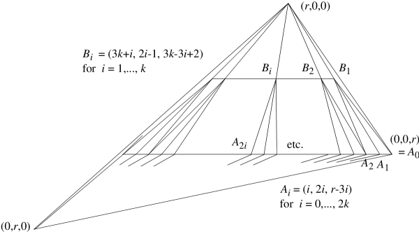
Figure 7: $\operatorname{{\mbox{$G$}}-Hilb}$ for $\frac{1}{r}(1,2,-3)$. $B_{i}$ is joined to $A_{2i-2},A_{2i-1},A_{2i}$

Sketch proof

Because ${\cal O}_{Z}=k[G]$ for $Z\in\operatorname{{\mbox{$G$}}-Hilb}$, for every character $a$ of $G$, the generators of $L(a)$ map surjectively to the 1-dimensional character space $k_{a}$, so there is a well defined ratio between the generators of ${\cal I}_{Z}(a)$. This means that for fixed $Z$ and every $L(a)$, we mark one monomial $s_{a}=x^{m(Z,a)}\in L(a)$ as the minimum of all the valuations $A_{1},\dots,A_{k}$ spanning a cone, and, using it as a generator, we get the invariant ratios $x^{m^{\prime}}/s_{a}$ as regular functions on $\operatorname{{\mbox{$G$}}-Hilb}$ near $Z$.

Example 6.2

Consider $\frac{1}{r}(1,2,-3)$ where $r=6k+1$. The quotient $X={\mathbb{C}}^{3}/({\mathbb{Z}}/r)$ is toric, and the $G$-Hilbert scheme is given by the triangulation of the first quadrant of Figure 7.

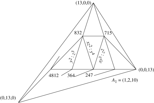
Figure 8: $\operatorname{{\mbox{$G$}}-Hilb}$ for $\frac{1}{13}(1,2,10)$: why join $(8,3,2)$—$(2,4,7)$?

This can be proved by carrying out the above proof explicitly. I omit the laborious details, concentrating on one point: how does the Hilbert scheme construction choose one triangulation in preference to another? For simplicity, consider only $r=13$, so the triangulation simplifies to Figure 8. How do I know to join $(8,3,2)$—$(2,4,7)$ by a cone $\sigma$, rather than $(7,1,5)$—$(3,6,4)$? By calculating $2\times 2$ minors of $\left(\begin{smallmatrix}8&3&2\\ 2&4&7\end{smallmatrix}\right)$, we see that the parameter on the corresponding line $E_{\sigma}\in Y$ should be the ratio $xz^{2}:y^{4}$, where $xz^{2},y^{4}\in L(8)$. The Newton polygon of $L(8)$ is

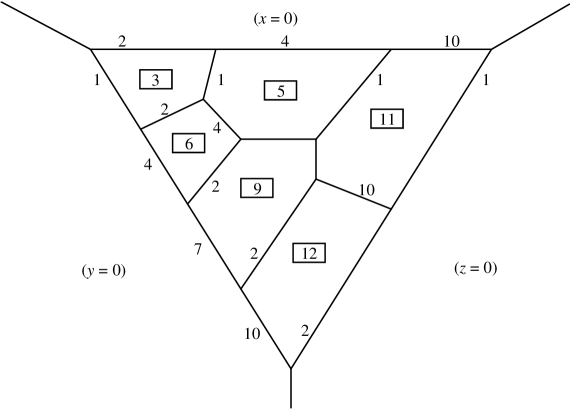
Figure 9: The McKay correspondence for $\frac{1}{13}(1,2,10)$

$$\begin{matrix}x^{8}&x^{6}y&x^{4}y^{2}&x^{2}y^{3}&y^{4}\\ &&\kern-28.45274pt(2,4,7)\kern-17.07182pt\\ &&xz^{2}&&y^{2}z^{3}\\ &&&\kern-28.45274pt(8,3,2)\kern-17.07182pt\\ &&&&z^{6}\end{matrix}$$

(The figure is not planar: $xz^{2}$ and $y^{4}$ are “lower”.) Here $(2,4,7)$ and $(8,3,2)$ have minima on the two planes as indicated, with common minima on $xz^{2}$ and $y^{4}$, so that the linear system $|xz^{2}:y^{4}|$ can be free on $L_{\sigma}$. But $(7,1,5)$ and $(3,6,4)$ don’t have a common minimimum here: $(7,1,5)$ prefers $y^{4}$ only, and $(3,6,4)$ prefers $xz^{2}$ only. If I join $(7,1,5)$—$(3,6,4)$, the linear system $|xz^{2}:y^{4}|$ would have that line as base locus.

The resolution is as in Figure 9. The McKay correspondence marks each exceptional stratum: a line $L$ parametrised by a ratio $x^{m_{1}}:x^{m_{2}}$ is marked by the common character space of $x^{m_{1}},x^{m_{2}}$. In other words, a linear system such as $xz^{2}:y^{4}$ corresponds to a tautological line bundle ${\cal L}(xz^{2}:y^{4})={\cal L}(8)$ with $c_{1}({\cal L}(8))\cdot L=1$.

The surfaces are marked by relations between the $c_{1}({\cal L}(i))$. In this case, because there are no hexagons, these all arise from surjective maps ${\cal O}_{X}(i)\otimes{\cal O}_{X}(j)\onto{\cal O}_{X}(i+j)$. For example, generators of the character spaces $1,2,3$ are given by monomials (written out as Newton polygons)

$$L(1):\enspace\begin{array}[]{lll}x&&y^{7}\\ &y^{2}z\\ z^{4}\end{array},\quad L(2):\enspace\begin{array}[]{llll}x^{2}&&y\\ xz^{4}\\ z^{8}\end{array}\quad\text{and}\quad L(3):\enspace\begin{array}[]{llll}x^{3}&xy&y^{8}\\ x^{2}z^{4}&y^{3}z\\ xz^{8}\\ z^{12}\end{array}\quad$$

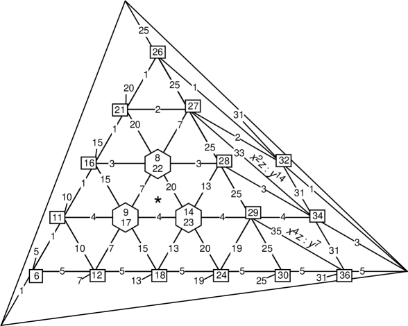
Figure 10: The McKay correspondence for $\frac{1}{37}(1,5,31)$

Clearly, $L(1)\otimes L(2)\onto L(3)$. (Thus this guy ${\cal L}(3)$ is not active in the resolution; in fact he’s completely useless, so deserves to be senior.) This means that on the resolution

$$c_{1}({\cal L}(3)-{\cal L}(1)-{\cal L}(2))=0,$$

and $c_{2}({\cal L}(3)-{\cal L}(1)-{\cal L}(2))$ is the dual class to the top left surface in Figure 9.

Example 6.3

The $G$-Hilbert scheme for $\frac{1}{37}(1,5,31)$ is given by the triangulation in Figure 10, which also indicates the labelling by characters of the McKay correspondence. I confine myself to a few comments: on the right-hand side,

$$(1,5,31)\text{--}(9,8,20)\quad \text{are joined by the ratio}\quad x^{4}z:y^{7}$$

$$(8,3,26)\text{--}(23,4,10)\quad \text{are joined by the ratio}\quad x^{2}z:y^{14}$$

for reasons similar to those explained in Example 6.2. The resolution has 3 regular hexagons (del Pezzo surfaces $S_{6}$), coming from the regular triangular pattern on the left-hand side of Figure 10. Tilings by regular hexagons appear quite often among the exceptional surfaces of the Hilbert scheme resolution $Y$, as we saw in Figure 3. The reason for this is taken up again at the end of §7, see Figure 13. The cohomology classes dual to these 3 surfaces are given as in (7) by taking $c_{2}$ of the relation $e_{1}+e_{2}+e_{3}-f_{1}-f_{2}$, where the $f_{1},f_{2}$ are the characters written in each little hexagonal box of Figure 10, and $e_{1},e_{2},e_{3}$ are the characters marking the 3 lines through the box. The relation $e_{1}+e_{2}+e_{3}=f_{1}+f_{2}$ can also be expressed as equality between two products of monomial ideals.

7 Nakamura’s proof that $\operatorname{{\mbox{$G$}}-Hilb}$ is a crepant resolution

Theorem 7.1 (Nakamura, very recent)

For $G$ a finite diagonal subgroup of $\operatorname{SL}(3,{\mathbb{C}})$, $Y=\operatorname{{\mbox{$G$}}-Hilb}\to X={\mathbb{C}}^{3}/G$ is a crepant resolution.

Proof

I start from the McKay quiver of $G$ with the 3 given characters $a,b,c$, corresponding to the eigencoordinates $x,y,z$, satisfying $a+b+c=0$; to get the full symmetry, draw this as a doubly periodic tesselation of the plane by regular hexagons, labelled by characters in $\widehat{G}$:

$$\setcounter{MaxMatrixCols}{15}\begin{matrix}&&&&&&&&&&&&&&\\[-18.0pt] &&&\kern-28.45274pt\cdots\kern-28.45274pt\\ &&&&\kern-28.45274pt2b\kern-28.45274pt\\ &&&&&\kern-28.45274ptb\kern-28.45274pt&&\kern-28.45274pta+b\kern-28.45274pt&&\kern-28.45274pt2a+b\kern-28.45274pt\\ \kern-28.45274pt\cdots\kern-28.45274pt&&\kern-28.45274pt2b+2c\kern-28.45274pt&&\kern-28.45274ptb+c\kern-28.45274pt&&\kern-28.45274pt0\kern-28.45274pt&&\kern-28.45274pta\kern-28.45274pt&&\kern-28.45274pt2a\kern-28.45274pt&&\kern-28.45274pt3a\kern-28.45274pt&&\kern-28.45274pt\cdots\kern-28.45274pt\\ &&&&&\kern-28.45274ptc\kern-28.45274pt&&\kern-28.45274pta+c\kern-28.45274pt\\ &&&&\kern-28.45274pt\cdots\kern-28.45274pt\end{matrix}$$ (11)

corresponding to the monomials

$$\setcounter{MaxMatrixCols}{13}\begin{matrix}&&&&&&&&&&&&\\[-18.0pt] &\kern-28.45274pt\cdots\kern-28.45274pt\\ &&\kern-28.45274pty^{2}\kern-28.45274pt\\ &&&\kern-28.45274pty\kern-28.45274pt&&\kern-28.45274ptxy\kern-28.45274pt&&\kern-28.45274ptx^{2}y\kern-28.45274pt\\ \kern-28.45274pty^{2}z^{2}\kern-28.45274pt&&\kern-28.45274ptyz\kern-28.45274pt&&\kern-28.45274pt1\kern-28.45274pt&&\kern-28.45274ptx\kern-28.45274pt&&\kern-28.45274ptx^{2}\kern-28.45274pt&&\kern-28.45274ptx^{3}\kern-28.45274pt&&\kern-28.45274pt\cdots\kern-28.45274pt\\ &&&\kern-28.45274ptz\kern-28.45274pt&&\kern-28.45274ptxz\kern-28.45274pt\\ &&\kern-28.45274pt\cdots\kern-28.45274pt\end{matrix}$$

For $\frac{1}{37}(1,5,31)$, we get Figure 11; it is a quiver, with arrows in the 3 principal directions “add 1, 5 or 31”. Or you can view it as the lattice of monomials modulo $xyz$, labelled with their characters in the $\frac{1}{37}(1,5,31)$ action; then the arrows are multiplication by $x,y,z$.

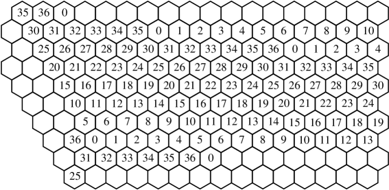
Figure 11: The McKay quiver for $\frac{1}{37}(1,5,31)$.

The whole of this business is contained one way or another in the hexagonal figure (11), together with its period lattice $\Pi$, and the many different possible ways of choosing nice fundamental domains for the periodicities; that is, we are doing Escher periodic jigsaw patterns on a fixed honeycomb background. First of all, note that the periodicity of (11) is exactly the lattice of invariant Laurent monomials modulo $xyz$. Call this $\Pi$.

The proof of Nakamura’s theorem follows from the following proposition:

Proposition 7.2

For every $G$-cluster $Z$, the defining equations (that is, the generators of ${\cal I}_{Z}$) can be written as 7 equations in one of the two following forms: either

$$\begin{matrix}x^{a+d+1}&=&\lambda y^{b}z^{f}\\ y^{b+e+1}&=&\mu z^{c}x^{d}\\ z^{c+f+1}&=&\nu x^{a}y^{e}\end{matrix}\qquad\begin{matrix}y^{b+1}z^{f+1}&=&\mu\nu x^{a+d}\\ z^{c+1}x^{d+1}&=&\lambda\nu y^{b+e}\\ x^{a+1}y^{e+1}&=&\lambda\mu z^{c+f}\end{matrix}\quad\text{and}\quad xyz=\lambda\mu\nu,$$

for some $a,b,c,d,e,f\geq 0$; or

$$\begin{matrix}x^{a+d}&=&\beta\gamma y^{b-1}z^{f-1}\\ y^{b+e}&=&\alpha\gamma z^{c-1}x^{d-1}\\ z^{c+f}&=&\alpha\beta x^{a-1}y^{e-1}\end{matrix}\qquad\begin{matrix}y^{b}z^{f}&=&\alpha x^{a+d-1}\\ z^{c}x^{d}&=&\beta y^{b+e-1}\\ x^{a}y^{e}&=&\gamma z^{c+f-1}\end{matrix}\quad\text{and}\quad xyz=\alpha\beta\gamma,$$

for some $a,b,c,d,e,f\geq 1$.

Proof of Theorem 7.1, assuming the proposition

Nakamura’s theorem follows easily, because $\operatorname{{\mbox{$G$}}-Hilb}$ is a union of copies of ${\mathbb{C}}^{3}$ with coordinates $\lambda,\mu,\nu$ (or $\alpha,\beta,\gamma$), therefore nonsingular. Every affine chart is birational to $X$, because it contains points with none of $\lambda,\mu,\nu=0$ (or none of $\alpha,\beta,\gamma=0$). Moreover, an easy linear algebra calculation shows that the equations ($\uparrow$) or ($\downarrow$) correspond to basic triangles of the junior simplex, so that each affine chart of $\operatorname{{\mbox{$G$}}-Hilb}$ is crepant over $X$. In more detail:

Case ($\uparrow$)

Write out the 3 x 3 matrix of exponents of the first three equations of ($\uparrow$):

$$\begin{matrix}a+d+1&-b&-f\\ -d&b+e+1&-c\\ -a&-e&c+f+1\end{matrix}$$

(note that each of the 3 columns add to 1, more less equivalent to the junior condition). The 2 x 2 minors of this give the 3 vertexes

$$P =(bc+bf+ef+b+c+e+f+1,\quad ac+cd+df+d,\quad ab+ae+de+a),$$

$$Q =(bc+bf+ef+b,\quad ac+cd+df+a+d+c+f+1,\quad ab+ae+de+e),$$

$$R =(bc+bf+ef+f,\quad ac+cd+df+b,\quad ab+ae+de+a+b+d+e+1).$$

The triangle PQR “points upwards”, in the sense that

$$P (1,0,0)$$ is closest to ,

$$Q (0,1,0)$$ is closest to ,

$$R (0,0,1)$$ is closest to .

The 3 given ratios $x^{a+d+1}:y^{b}z^{f}$, etc. correspond to the 3 sides of triangle $PQR$. In any case, all the vertexes belong to the junior simplex, so that this piece of $\operatorname{{\mbox{$G$}}-Hilb}$ is crepant over $X$.

Case ($\downarrow$)

Write out the exponents of the second set of three equations:

$$\begin{matrix}-(a+d)+1&b&f\\ d&-(b+e)+1&c\\ a&e&-(c+f)+1\end{matrix}$$

again, each of the 3 columns add to 1, and the $2\times 2$ minors of this give the 3 vertexes

$$P =(bc+bf+ef-b-c-e-f+1,ac+cd+df-d,ab+ae+de-a),$$

$$Q =(bc+bf+ef-b,ac+cd+df-a-d-c-f+1,ab+ae+de-e),$$

$$R =(bc+bf+ef-f,ac+cd+df-b,ab+ae+de-a-b-d-e+1),$$

all of which again belong to the junior simplex, so this affine chart is also crepant over $X$. This time the triangle $PQR$ “points downwards”, in the sense that

$$P (1,0,0)$$ is furthest from ,

$$Q (0,1,0)$$ is furthest from ,

$$R (0,0,1)$$ is furthest from .

The 3 given ratios $x^{a+d-1}:y^{b}z^{f}$, etc. again correspond to the 3 sides. Q.E.D. for the theorem, assuming the proposition.

Proof of Proposition 7.2

Most of this is very geometric: any reasonable choice of monomials in $x,y,z$ whose classes in ${\cal O}_{Z}$ form a basis is given by a polygonal region $M$ of the honeycomb figure (11) satisfying 2 conditions:

1. in each of the 3 triants (triangular sector) it is concave, that is, a downwards staircase: because it is a Newton polygon for an ideal;

2. it is a fundamental domain of the periodicity lattice $\Pi$: because we assume that ${\cal O}_{Z}=k[G]$, therefore every character appears exactly once.

The condition (ii) means that $M$ and its translates by $\Pi$ tesselate the plane, so they form a kind of jigsaw pattern like the Escher periodic patterns. However, in each of the 3 principal directions corresponding to the $a$, $b$, and $c$-axes, there is only one acute angle, namely the summit at the end of the $a$-axis (etc.). Therefore $M$ can only have one valley (concave angle) in the $b,c$ triant. As a result, there is only one geometric shape for the polygon $M$, the tripod or mitsuya (3 valleys, or 3 arrows) of Figure I.

I introduce some terminology: the tripod $M$ has 3 summits at the end of the axis of monomials $x^{i}$, and 3 triants or sectors of $120^{\circ}$ containing monomials $x^{i}y^{j}$. Each triant has one valley and two shoulders (incidentally, the 6 shoulders give the socle of ${\cal O}_{Z}$).

Remark 7.3

There are degenerate cases when some of the valleys or summits are trivial (for example, $a=0$ in $\uparrow$). The most degenerate case is a straight lines, when ${\cal O}_{Z}$ is based by powers of $x$ (say), and the equations boil down to $y=x^{i},z=x^{j}$ (the $x$-corner of the resolution). I omit discussion of these cases, since the equations of the cluster $Z$ are always a lot simpler.

      I o o o
     o I o o o
    o o I o o o
     o o I o o o o o o
      o o I o o o o o o
     o o o I I I I I I I     (Figure I)
    o o o I o o o o o o
     o o I o o
      o I o o
       I o o

Thus there is only one “geometric” solution to the Escher jigsaw puzzle, namely

               ...  I I I I I I I I I I
              u u u I u u u u u u u u u u u
               u u I u u
      I o o o   u I u u
     o I o o o   I u u    I v v v
    o o I o o o          v I v v v
     o o I o o o o o o  v v I v v v
      o o I o o o o o o  v v I v v v v v v ...   (Figure II)
     o o o I I I I I I I  v v I v
    o o o I o o o o o o  v v ...
     o o I o o          v v
      o I o o
       I o o

In particular, the external sides (going out to the 3 summits) are equal plus-or-minus 1 to the opposite internal sides (going in to the 3 valleys).

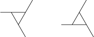
Figure 12: Two different cocked hats

However, the geometric statement of Figure II is only exact for closed polygons, whereas our tripods are Newton polygons spanned by integer points, and are separated by a thin “demilitarised zone” between the integer points. When you consider the tripods together with the integer lattices, there are two completely different ways in which the three shoulders of neighbouring tripods can fit together (corresponding to the two cyclic orders, or the two cocked hats of Figure 12), namely either ($\uparrow$)

        y y y y z
         y y y z
        x x x z z
         x x x z z

where the last $\tt y$ is just after the last $\tt x$, and the shoulder of the $\tt z$ is level with the top row of $\tt x$

or ($\downarrow$)

        y y y z z
         y y z z
        x x x z z
         x x x z z

where the last $\tt y$ is just before the last $\tt x$ and the top row of $\tt x$ is just below the shoulder of the $\tt z$.

The two different forms ($\uparrow$) and ($\downarrow$) come from this patching.

Remark 7.4 (Algorithm for $\operatorname{{\mbox{$G$}}-Hilb}$)

Nakamura [N3] gives an algorithm to compute $\operatorname{{\mbox{$G$}}-Hilb}$ in this case as a toric variety. This can be viewed as a way of classifying all the possible tripods in terms of elementary operations, which correspond to the 0-strata and the 1-strata of the toric variety $\operatorname{{\mbox{$G$}}-Hilb}$. You pass from an $\uparrow$ tripod to a $\downarrow$ one by shaving off a layer of integer points one thick around one valley (assumed to have thickness $\geq 1$), and glueing it back around the opposite summit. And vice versa to go from $\downarrow$ to $\uparrow$. You can start from anywhere you like, for example from the $x$-corner (see Remark 7.3).

Nakamura’s algorithm applied to the statement in Proposition 7.2 expressed in terms of the fan triangulating the junior simplex, gives that if $\uparrow$ and $a,b,c,d,\allowbreak e,f\geq k\geq 2$ (say) then you can cross any wall of the “upwards” triangle of the fan to get a new $\downarrow$ coordinate patch with $a^{\prime},b^{\prime},c^{\prime},d^{\prime},e^{\prime},f^{\prime}\geq k-1$, which corresponds to a “downwards” triangle, and vice-versa. It follows that the first triangle is surrounded by a patch of width $k-1$ which is triangulated by the regular triangular lattice, so that the resolution has a corresponding patch of regular hexagons (that is, del Pezzo surfaces of degree 6). Figure 11 shows the McKay quiver of $\frac{1}{37}(1,5,31)$ and Figure 13 its fundamental domain giving the equations of $G$-clusters

$$x^{4}=\lambda y^{2}z,\quad y^{4}=\mu xz^{3},\quad z^{5}=\nu x^{2}y,\quad\text{etc.}$$

on the coordinate chart of the resolution of $\frac{1}{37}(1,5,31)$, corresponding to the starred triangle of Figure 10.

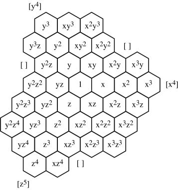
Figure 13: A fundamental domain of the McKay quiver for $\frac{1}{37}(1,5,31)$

References

- [B] Jean-Luc Brylinski, A correspondence dual to McKay’s, preprint, alg-geom/9612003
- [C] P. Candelas, X.C. de la Ossa, P.S. Green and L. Parkes, A pair of Calabi–Yau manifolds as an exactly soluble superconformal theory, Nuclear Phys. B 357 (1991), 21–74
- [DHZ] D. Dais, M. Henk and G. Ziegler, All Abelian quotient c.i. singularities admit projective crepant resolutions in all dimensions, Max Planck Inst. preprint MPI 97–4.
- [GK] V. Ginzburg and M. Kapranov, Hilbert schemes and Nakajima’s quiver varieties, unpublished notes, May 1995
- [GSp-V] G. Gonzales-Sprinberg and J.-L. Verdier, Construction géométrique de la correspondance de McKay, Ann. sci. ENS 16 (1983), 409–449
- [HH] F. Hirzebruch and H. Höfer, On the Euler number of an orbifold, Math. Ann. 286 (1990), 255–260
- [I1] Y. Ito, Crepant resolutions of trihedral singularities and the orbifold Euler characteristic, Intern. J. Math. 6 (1995), 33–43
- [I2] Y. Ito, Gorenstein quotient singularities of monomial type in dimension three, J. Math. Sci. Univ. of Tokyo 2, (1995), 419–440
- [IN1] Y. Ito and I. Nakamura, McKay correspondence and Hilbert schemes, Proc. Japan Acad. 72 (1996), 135–138
- [IN2] Y. Ito and I. Nakamura, Hilbert schemes and simple singularities and , Hokkaido Univ. preprint #348, 1996, 22 pp.
- [IN3] Y. Ito and I. Nakamura, The coinvariant algebra and quivers of a simple singularity (in preparation)
- [IR] Y. Ito and M. Reid, The McKay correspondence for finite subgroups of , in Higher Dimensional Complex Varieties (Trento, Jun 1994), M. Andreatta and others Eds., de Gruyter, Mar 1996, 221–240
- [McK] J. McKay, Graphs, singularities and finite groups (Proc. Symp. in Pure Math, 37, 1980, 183–186
- [N] H. Nakajima, Lectures on Hilbert schemes of points on surfaces, Univ. of Tokyo preprint, Preliminary version, Oct 1996, available from http://www.math.tohoku.ac.jp/tohokumath/nakajima/TeX.html
- [N1] I. Nakamura, Simple singularities, McKay correspondence and Hilbert schemes of -orbits, preprint
- [N2] I. Nakamura, Hilbert schemes and simple singularities , and , Hokkaido Univ. preprint #362, 1996, 21 pp.
- [N3] I. Nakamura, Hilbert schemes of -orbits for Abelian (in preparation)
- [YPG] M. Reid, Young person’s guide to canonical singularities, in Algebraic Geometry, Bowdoin 1985, ed. S. Bloch, Proc. of Symposia in Pure Math. 46, A.M.S. (1987), vol. 1, 345–414
- [R] O. Riemenschneider, Deformationen von Quotientensingularitäten (nach zyklischen Gruppen), Math. Ann. 209 (1974) 211–248
- [Roan] S-S. Roan, On resolution of quotient singularity, Intern. J. Math. 5 (1994), 523–536