[adap-org/9907010] 1 An example of the time evolution of a single species (inset) from a population of 𝑁=5000 individuals and 𝑆=300 species in the pool. Here 𝐶=0.5 and 𝜇=5×10⁻³. We can see a wide spectrum of fluctuations in 𝑛⁢(𝑡). Main figure: the number of species present in the simulated ecosystem increases up to an average value <𝑆>≈125 imposed by the matrix connectivity.

Scaling in a Multispecies

Network Model Ecosystem

Ricard V. Solé^1,2, David Alonso^1,3 and Alan McKane⁴

(1) Complex Systems Research Group

Department of Physics, FEN, Universitat Politècnica de Catalunya

Campus Nord B4, 08034 Barcelona, Spain

(2) Santa Fe Institute, 1399 Hyde Park Road, New Mexico 87501, USA

(3) Department of Ecology, Facultat de Biologia, Universitat de Barcelona

Diagonal 645, 08045 Barcelona, Spain

(4) Department of Theoretical Physics, University of Manchester

Manchester M13 9PL, UK

Abstract

A new model ecosystem consisting of many interacting species is introduced. The species are connected through a random matrix with a given connectivity $C_{\pi}$ . It is shown that the system is organized close to a boundary of marginal stability in such a way that fluctuations follow power law distributions both in species abundance and their lifetimes for some slow-driving (immigration) regime. The connectivity and the number of species are linked through a scaling relation which is the one observed in real ecosystems. These results suggest that the basic macroscopic features of real, species-rich ecologies might be linked with a critical state. A natural link between lognormal and power law distributions of species abundances is suggested.

Submitted to Physical Review Letters

PACS number(s): 87.10.+e, 05.40.+j, 05.45.+b

The universal properties of complex biosystems have attracted the attention of physicists over the last decade or so. The standard approach to complex ecosystems is based on the classical Lotka-Volterra (LV) $S$ -species model [1]:

{dN_{i}\over dt}=N_{i}\Biggl{(}\epsilon_{i}-\sum_{j=1}^{S}\alpha_{ij}N_{j}(t)\Biggl{)}\ ,

(1)

where $\{N_{i}\};(i=1,...,S)$ is the population size of each species. Here $\epsilon_{i}$ and $\alpha_{ij}$ are constants that introduce feedback loops and interactions among different species. The matrix ${\bf A}=(\alpha_{ij})$ describes the interaction graph [1] and even a small degree of asymmetry leads to very complicated dynamics, although several generic properties have been identified. In this respect, recent studies on a related class of replicator equations, where an initial random graph evolves towards a highly non-random network, revealed remarkable self-organized features [2].

A classical result on randomly wired ecosystems [3] shows that a critical limit to the number of species $S$ exists for a given connectivity $C$ . Here $C$ is the fraction of non-zero matrix elements. This limit is sharp (a phase transition): below the critical value the system is stable but it becomes unstable otherwise. The basic inequality is that the community will be stable if $C\leq\sigma/S$ , where $\sigma$ is a given constant. Here the equality defines the boundaries between the stable and the unstable domains. Field studies show that, in general, $C=\sigma S^{-1+\epsilon}$ with $\epsilon\in[0,1/2]$ [4].

More recently some authors have suggested that complex biosystems could be self-organized into a critical state [5,6]. Most of these approaches based on self-organized criticality (SOC), such as the Bak-Sneppen model [5], involve a time scale that is assumed to be very large. But the species properties of a given ecosystem do not change appreciably on a smaller time scale [7] and several field observations suggest that real ecosystems display some features characteristic of SOC states. In particular: (i) the analysis of time series [8] shows that the largest Lyapunov exponent is typically close to zero; (ii) studies on colonization in islands show that after a critical number of species is reached, extinction events are triggered, following a power law distribution [9]; (iii) the lifetime distribution of species (defined in terms of local extinction in given areas) is also a power law $N(T)\approx T^{-\theta}$ with $\theta=1.12$ [9] to $\theta=1.6$ [10] and (iv) in species-rich ecosystems, the number of species $N_{s}(n)$ with $n$ individuals is also a power law $N_{s}(n)\approx n^{-\gamma}$ , where $\gamma$ is close to one, although log-normal distributions with long tails are also well known [11]. But none of these observations (together with the $C-S$ law) have been explained within a single theoretical framework.

Refer to caption — Figure 1: An example of the time evolution of a single species (inset) from a population of $N=5000$ individuals and $S=300$ species in the pool. Here $C=0.5$ and $\mu=5\times 10^{-3}$ . We can see a wide spectrum of fluctuations in $n(t)$ . Main figure: the number of species present in the simulated ecosystem increases up to an average value $<S>\approx 125$ imposed by the matrix connectivity.

In this letter we present a new model which can be used as a simple alternative to the LV formulation and follows the simple (but somewhat different) approach of other studies on random graphs [2]. The model involves a set $\Theta_{s}$ of $S$ (possible) species and a population size $N$ . Individuals of different species interact through a matrix $\bf\Omega$ , with a pre-defined connectivity $C_{\pi}\in[0,1]$ . The $\Omega_{ij}$ are randomly chosen from a uniform distribution $\rho(x)$ . Each time step two individuals are taken at random belonging, say, to species $i$ and $j$ respectively. Then if $\Omega_{ij}>\Omega_{ji}$ the individual belonging to $j$ is replaced, with probability $1-\mu$ , by a new individual of species $i$ . If $\Omega_{ij}=\Omega_{ji}=0$ then nothing happens. This rule is repeated $N$ times and these $N$ updates define our time step. Additionally, with probability $\mu$ , any individual can be replaced by another individual of any of the species from $\Theta_{s}$ . These rules makes our model close to equation (1) when $\alpha_{ij}>0$ ( $S$ -species competition model [1]). So two basic reactions are allowed: (i) interaction through $\bf\Omega$ and (ii) random replacement by a new species from the $\Theta_{s}$ pool. The second rule introduces immigration (at a rate $\mu$ ): our driving force [12,13].

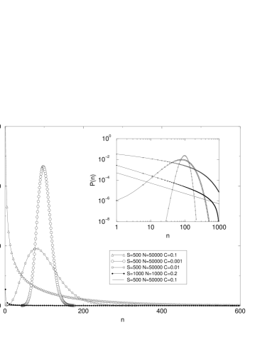
An example of the temporal dynamics of this model is shown in figure 1, where we can see a wide spectrum of fluctuation sizes, not very different from those observed in some natural communities [1,8]. Starting from any given initial number of species, this model self-organizes towards a subset of species (with average $<S>$ ). The specific subset itself changes in time. Let $C^{*}$ be the probability of having two species connected. Then $C^{*}$ and $<S>$ are linked by a power law $<S>=k(C^{*})^{-1+\epsilon(\mu)}$ . Once this $<S>$ is reached, complex fluctuations can arise and under some conditions (see below) power laws are observable. The analysis of the population fluctuations typically shows, for small driving $\mu$ and large enough $C_{\pi}$ , a power law $P(n)\approx n^{-\gamma}f_{\mu}(n)$ . Here $\gamma=1$ when $N\gg S\gg 1$ and $f_{\mu}(n)$ an exponential cut-off. The lifetime distribution of species is also a power law: $N(T)\approx T^{-\theta}$ and for $N\gg S$ , $\theta\in(1,3/2)$ . The $\theta=3/2$ limit corresponds to low-level connectivities (i.e. random-walk-like behavior) and $\theta=1$ to the situation were interactions dominate over immigration. It is remarkable that these limits in the lifetimes correspond to those reported from field studies [9,10].

The limiting case for $\mu\rightarrow 0$ shows the exact hyperbolic relation and can be derived from a mean-field approach. It is not difficult to see that the number of species will change in time following:

{dS\over dt}=\mu N-C^{*}S\ ,

(2)

where the first term on the right-hand side stands for the continuous introduction of new species at a rate $\mu$ and the second for the instability derived from interactions. The previous equation gives an exponential approach to criticality $S(t)=[\mu N-(\mu N-C^{*}S(0))e^{-C^{*}t}]/C^{*}$ which leads at the steady state to

S^{*}={\mu N\over C^{*}}\propto{1\over C^{*}}\ .

(3)

A mean field theory of species abundance can be derived. Let us start with the master equation for this model. If $P(n,t)$ is the probability (for any species) of having $n$ individuals at time t, the one-step process is described by [14]:

{dP(n,t)\over dt}=r_{n+1}P(n+1,t)+g_{n-1}P(n-1,t)-(r_{n}+g_{n})P(n,t)\ ,

(4)

where the one-step transition rates are:

r_{n}\equiv W(n-1|n)=C^{*}(1-\mu){n\over N}{N-n\over N-1}+{\mu\over S}(S-1){n\over N}\ ,

(5)

g_{n}\equiv W(n+1|n)=C^{*}(1-\mu){n\over N}{N-n\over N-1}+{\mu\over S}(1-{n\over N})\ .

(6)

From (5) and (6) we see that $r_{0}=0$ and $g_{N}=0$ and we define $g_{-1}=0$ and $r_{N+1}=0$ . The stationary distribution $P_{s}(n)$ is obtained from $dP(n)/dt=0$ using standard methods [14] namely by writing

P_{s}(n)={g_{n-1}\,g_{n-2}...\,g_{0}\over r_{n}\,r_{n-1}...\,r_{1}}P_{s}(0)\ ,

(7)

and using the normalization condition $\sum_{n=0}^{N}P_{s}(n)=P_{s}(0)+\sum_{n>0}P_{s}(n)=1$ , to show that

(P_{s}(0))^{-1}=\sum_{n=0}^{N}{N\choose n}(-1)^{n}{\Gamma(n+\lambda^{*})\over\Gamma(\lambda^{*})}{\Gamma(1-\nu^{*})\over\Gamma(n+1-\nu^{*})}\ .

(8)

Here $\lambda^{*}=\mu^{*}(N-1)$ and $\nu^{*}=N+\mu^{*}(N-1)(S-1)$ , where $\mu^{*}=\mu/[(1-\mu)SC^{*}]$ . This sum takes the form of a Jacobi polynomial $P_{N}^{(\alpha,\beta)}(x)$ [15], with $\alpha=-\nu^{*}$ , $\beta=\lambda^{*}+\nu^{*}-(N+1)$ and $x=-1$ , which can itself be expressed in terms of gamma functions for this value of $x$ . Therefore using $\beta(p,q)=\Gamma(p)\Gamma(q)/\Gamma(p+q)$ , the stationary, normalized solution can be written in the form [16]

P_{s}(n)={N\choose n}{\beta(n+\lambda^{*},\nu^{*}-n)\over\beta(\lambda^{*},\nu^{*}-N)}\ .

(9)

As the connectivity (or the immigration rate) increases, the distributions changes from Gaussian to lognormal and to power laws (fig. 2). This is expected since very small connectivities will make interactions irrelevant, with fluctuations dominated by random events. We can simplify (9) in the region of interest: $N$ and $S$ large, and $N\gg n_{max}$ where $n=1,...,n_{max}$ . If in addition $\lambda\ll 1$ , which corresponds to $\mu$ small: $\mu\ll SC^{*}/N$ , we get a scaling relation:

P_{s}(n)={\cal K}n^{-1}\exp(-n\mu^{*}S)\ ,

(10)

where ${\cal K}=(\mu^{*}S)^{\lambda^{*}}/\Gamma(\lambda^{*})$ in agreement with simulations and field data. These results suggest a simple link between a range of statistical distributions from those generated by multiplicative events to those related with SOC dynamics.

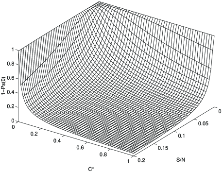
From this solution we can compute the stationary number of species $<S>=(1-P(0))S$ and find the relation between this quantity and the probability of having two species connected, $C^{*}$ . Under the same conditions that led to (10), we find that $P_{s}(0)=(\mu^{*}S)^{\lambda^{*}}$ [17] which in this parameter range gives $<S>=S\mu^{*}N\ln(1/(\mu^{*}S)$ . Substituting in the expression for $\mu^{*}$ gives

<S>={\mu N\over(1-\mu)C^{*}}\Bigl{[}\ln\Bigl{(}{1-\mu\over\mu}\Bigr{)}+\ln C^{*}\Bigr{]}\approx{\cal A}(C^{*})^{-1+\epsilon(\mu)}\ ,

(12)

where $\epsilon$ is given by $\epsilon^{-1}=\ln((1-\mu)/\mu)\approx\ln\mu^{-1}$ and ${\cal A}$ is a constant equal to $N\epsilon^{-1}\exp(-\epsilon^{-1})$ . The additional conditions under which (12) hold are $\lambda^{*}\ll\epsilon$ and $|\ln(C^{*})|\ll|\ln(\epsilon)|$ . The latter means that $C^{*}$ may not be taken too small, for example, if $\mu\approx 10^{-5}$ then $C^{*}\geq 0.1$ . With these values the former condition is satisfied if $N/S$ is not too large. Thus (12) holds for a wide range of parameter values. The relation between $<S>$ and $C^{*}$ is shown in figure 3 for different $S/N$ values and a quite large immigration rate ( $\mu=10^{-3}$ ). In this case, the hyperbolic relation is only reached for large $S/N$ and for smaller $S/N$ values, slower decays (i. e. $<S>\approx C^{-1+\epsilon}$ ) are obtained [18].

In summary, a simple $S$ -species network model that shows both lognormal (even Gaussian) distributions as well as SOC dynamics has been introduced. Starting from random initial conditions, the system evolves towards a state characterized by some well-defined scaling laws and statistical features. High immigration, small $S/N$ relations or low connectivities lead to lognormal distributions. These are replaced by well-defined power laws as the interactions become more relevant. In the last case, a multiplicity of metastable states, the presence of a threshold in the number of species $S_{c}=<S>$ , the scale separation between the driving when $\mu$ is small and the system response fully describe our system as SOC. As a consequence of critical dynamics several well-known field observations are recovered. The interpretation of this model provides a new framework for understanding how complex dynamics emerge in multispecies ecosystems and suggest that some well-known time series from natural communities would be the result of criticality instead of deterministic chaotic behavior.

Acknowledgments

The authors thank H. Jensen, R. Engelhardt, S. Pimm, S. Jain, S. Kauffman and K. Sneppen for useful comments. Special thanks to Per Bak for encouraging comments. This work has been supported by a grant PB97-0693 and by the Santa Fe Institute (RVS), CIRIT 99 (DA) and EPSRC grant GR/K79307 (AM).

1 References

1.

R. M. May, Stability and complexity in model ecosystems. Princeton U. Press, Princeton (1973); N. S. Goel, S. C. Maitra and E. W. Montroll. Rev Mod. Phys 65, 231 (1971)
2.

S. Jain and S. Krishna, preprint adap-org/9810005, to appear in Phys. Rev. Lett.; see also: adap-org/9809003.
3.

R. M. May, Nature 238, 413 (1972); see also T. Hogg, B. Huberman and J. M. McGlade, Proc. R. Soc. London B237, 43 (1989). Specifically, if $P(S,C,\sigma)$ is the probability that the system is stable for a given $(S,C,\sigma)$ set, where $\sigma$ is the matrix variance, we have (for large $S$ ) $P(S,C,\sigma)\rightarrow 1$ if $CS\leq\sigma$ and $P(S,C,\sigma)\rightarrow 0$ otherwise.
4.

S. Pimm, The Balance of Nature, Chicago U. Press, 1994
5.

P. Bak, and K. Sneppen, Phys. Rev. Lett. 71, 4083 (1993)
6.

R. V. Solé and S. C. Manrubia, Phys. Rev. E54, R42-R45 (1996); R. Engelhardt, Emergent Percolating Nets in Evolution, Ph.D. Thesis, University of Copenhagen, Denmark, 1998
7.

J. Maynard Smith and N. C. Stenseth, Evolution 38, 870 (1984). The ecological time scale involves changes in population sizes and local extinction and immigration, but a conserved number of species. The evolutionary time scale deals with extinction and speciation events.
8.

S. Ellner and P. Turchin, Am. Nat. 145, 343 (1995)
9.

T. H. Keitt, and P. S. Marquet, J. Theor. Biol. 182, 161 (1996)
10.

T. H. Keitt and H. E. Stanley, Nature 393, 257 (1998)
11.

E. C. Pielou, An Introduction to Mathematical Ecology. Wiley, 1969; Some recent, extensive field data analysis from marine ecosystems has shown that this communities follow very well-defined power law in species abundances with $N_{s}(n)\approx n^{-\gamma}$ with $\gamma\in(1,1.25)$ spanning three to four decades (S. Pueyo, unpublished data)
12.

R. V. Solé and D. Alonso, Adv. Complex Systems 1, 203 (1998)
13.

Immigration is the main external source of perturbation in ecosystems not influenced by strong climate fluctuations.
14.

N. G. Van Kampen, Stochastic Processes in Physics and Chemistry, Elsevier, 1981; C. W. Gardiner, Handbook of Stochastic Methods (2nd edition). Springer, Berlin (1990)
15.

M. Abramowitz and A. Stegun (eds), Handbook of Mathematical Functions, Dover, New York 1965.
16.

In various intermediate expressions we have assumed that $\nu^{*}$ is not an integer, but this final result is well defined for all meaningful ranges of the parameters.
17.

Since $P_{s}(0)=(S-1)/S$ , for $\lambda^{*}$ approaching zero, (12) should be approximated by $P_{s}(0)=((S-1)/S)(\mu^{*}S)^{\lambda^{*}}$ . Then, instead of (12), a correction is needed when $\lambda^{*}$ is tending to zero: $<S>-1={\cal A}[C^{*}]^{-1+\epsilon(\mu)}$ . As $\mu$ is tending to zero, $<S>=1$ , for high connectivities.
18.

In (12), $C^{*}$ appears instead of the fraction of non-zero elements of the connectivity matrix, $C_{\pi}$ . Both connectivities have exactly the same meaning, i.e. the probability of having two species connected, as long as completely asymmetrical interaction between species is forbidden. If $\Omega_{ij}$ (the effect of $j$ on $i$ species) is non-zero, then $\Omega_{ji}$ may be extremely low but different from zero. The former assumption is very realistic in natural communities.