Metastable Evolutionary Dynamics:
Crossing Fitness Barriers or
Escaping via Neutral Paths?

Abstract

We analytically study the dynamics of evolving populations that exhibit metastability on the level of phenotype or fitness. In constant selective environments, such metastable behavior is caused by two qualitatively different mechanisms. One the one hand, populations may become pinned at a local fitness optimum, being separated from higher-fitness genotypes by a fitness barrier of low-fitness genotypes. On the other hand, the population may only be metastable on the level of phenotype or fitness while, at the same time, diffusing over neutral networks of selectively neutral genotypes. Metastability occurs in this case because the population is separated from higher-fitness genotypes by an entropy barrier: The population must explore large portions of these neutral networks before it discovers a rare connection to fitter phenotypes.

We derive analytical expressions for the barrier crossing times in both the fitness barrier and entropy barrier regime. In contrast with “landscape” evolutionary models, we show that the waiting times to reach higher fitness depend strongly on the width of a fitness barrier and much less on its height. The analysis further shows that crossing entropy barriers is faster by orders of magnitude than fitness barrier crossing. Thus, when populations are trapped in a metastable phenotypic state, they are most likely to escape by crossing an entropy barrier, along a neutral path in genotype space. If no such escape route along a neutral path exists, a population is most likely to cross a fitness barrier where the barrier is narrowest, rather than where the barrier is shallowest.

Santa Fe Institute Working Paper 99-07-041

Keywords: Populations dynamics, neutral networks,

fitness barrier, entropy barrier, metastability.

Running Head: Metastable Evolutionary Dynamics

Contents

toc

I Introduction

For populations evolving under selection, mutation, and a static fitness function, there are two main mechanisms thought to be responsible for the occurrence of dynamical metastability—a behavior commonly observed in natural and artificial evolutionary processes [1, 2, 3, 8, 10, 23] and called punctuated equilibria in paleobiology [13]. First, a population may become trapped around a local optimum in the fitness “landscape” until a rare mutant crosses a fitness barrier to a higher nearby peak. Second, more recently it has been proposed [10, 15, 29] that populations may evolve neutrally, drifting randomly over neutral networks of isofitness genotypes in genotype space, until a rare single-point mutant connection is found to another neutral network of higher fitness. In this case, the population must cross an entropy barrier by visiting a large volume of the neutral network before it discovers a path to higher fitness.

To understand the relative roles of these two mechanisms in evolutionary metastability, in the following we study the dynamics of a population evolving under simple fitness functions that contain a single fitness barrier of tunable height and width. In order for the population to escape its current metastable state and so reach higher fitness, it must create a genotype that is separated from the current fittest genotypes in the population by a valley of lower-fitness genotypes. The height of the fitness barrier measures the relative selective difference between the current fittest genotypes and the lower-fitness genotypes in the intervening valley. Its width denotes the number of point mutations the current fittest genotypes must undergo to cross the valley of low fitness genotypes. We derive explicit analytical predictions for the barrier crossing times as a function of population size, mutation rate, and barrier height and width. The scaling of the fitness-barrier crossing time as a function of these parameters shows that the waiting time to reach higher fitness depends crucially on the width of the barrier and much less on the barrier height.

This contrasts with the scaling of the barrier crossing time for a particle diffusing in a double-well potential—a model proposed previously for populations crossing a fitness barrier [20, 22]. For such stochastic processes, it is well known that the waiting time scales exponentially with the barrier height [12]. In the population dynamics that we analyze here, we find that the waiting time scales approximately exponential with barrier width and only as a power law of the logarithm of barrier height. In addition, the waiting time scales roughly as a power law in both population size and mutation rate.

When the barrier height is lowered below a critical height, the fitness barrier turns into an entropy barrier. We show that, in general, neutral evolution via crossing entropy barriers is faster by orders of magnitude than fitness barrier crossing. Additionally, we show that the waiting time for crossing entropy barriers exhibits anomalous scaling with population size and mutation rate.

Finally, we extend our analysis to a class of more complicated fitness functions that contain a network of tunable fitness and entropy barriers. We show that the theory still accurately predicts fitness- and entropy-barrier crossing times in these more complicated cases.

The general conclusion drawn from our analysis is that, when populations are trapped in a metastable phenotypic state, they are most likely to escape this metastability by crossing an entropy barrier. That is, the escape to a new phenotype occurs along a neutral path in genotype space. If no such neutral path exists, then the population is most likely to cross a fitness barrier at the place where the barrier is narrowest.

A Evolutionary Pathways and Metastability

The notion of an adaptive landscape, first introduced by Wright [32], has had a large impact on our appreciation of the mechanisms that control how populations evolve in static environments. The intuitive idea is that a population moves up the slopes of its fitness “landscape” just as a physical system moves down the slope of its potential-energy surface. Once this analogy has been accepted, it is natural to borrow many of the qualitative results on the dynamics of physical systems to account for the dynamics of evolving populations. For instance, it has become common to assume that an evolving population can be modeled by a single uphill walker in a “rugged” fitness landscape [16, 21].

There are, however, seemingly different kinds of evolutionary behavior than incremental adaptation via “landscape” crawling. For example, metastability or punctuated equilibrium of phenotypic traits in an evolving population appears to be a common occurrence in biological evolution [8, 13] as well as in models of natural and artificial evolution [1, 3, 10]. As just pointed out, for simple cases where populations evolve in a relatively constant environment, there are two main mechanisms that have been proposed to account for this type of metastable behavior.

The first and most commonly accepted explanation was already implicit in Wright’s shifting balance theory [33]. A population moves up the slope of its fitness “landscape” until it reaches a local optimum, where it stabilizes. The population is pictured as a cloud in genotype space focused around this local optimum. The population remains in this state until a rare sequence of mutants crosses a valley of low fitness towards a higher fitness peak. In this view, metastability is the result of fitness barriers that separate local optima in genotype space.

This mechanism for metastability is very reminiscent of that found in physical systems. Metastability occurs there because local energy minima in state space are separated by potential energy barriers, which impede the immediate transition between the minima. A physical system generally moves through its state space along trajectories that lower its energy. Once it reaches a local minimum it tends to stay there. However, when such a system is subject to thermal fluctuations, through a sequence of chance events it can eventually be pushed over a barrier that separates the current local minimum from another. When this transition occurs, it turns out that the system moves quickly to the new local minimum.

Mathematically, barrier crossing processes in physical systems are most often described as diffusion in a potential field, where the potential represents the energy “landscape”. These processes have been extensively studied and the basic quantitative results are widely known [11, 12, 26]. For example, barrier crossing times increase exponentially with the height of the barrier and inverse exponentially with the fluctuation amplitude, as measured by temperature.

In light of the physical metaphor for evolving populations, it is not surprising that the dynamics of populations crossing fitness barriers has been modeled using a class of diffusion equations analogous to those used to describe thermally driven systems in a potential [20, 22]. In this approach, the dynamics of the average fitness of the population is modeled as diffusion over the “fitness landscape”, thermal fluctuations are replaced by random genetic mutations and drift, and the population size, which controls sampling stochasticity, plays the role of inverse temperature. As a direct consequence, it was found that fitness-barrier crossing times scale exponentially with population size in these models. Note that it is assumed in this approach that the population as a whole must cross the fitness barrier.

In the following, we show that the analogy with the physical situation and, in particular, the translation of results from there are misleading for the understanding of the evolutionary dynamics. For example, a direct analysis of the population dynamics reveals that for most parameter ranges, the time to cross a fitness barrier scales very differently for populations evolving under selection and mutation. For example, the waiting time is determined by how long it takes to generate a rare sequence of mutants that crosses the fitness barrier, as opposed to how long it takes the population as a whole to cross the fitness barrier.

This brings us to the second main mechanism for metastability—one that has been put forward more recently [2, 10, 15, 23, 29]. The second mechanism derives from the observation that large sets of mutually fitness-neutral genotypes are interconnected along single-point mutation paths. That is, sets of isofitness genotypes form extended neutral networks under single-point mutations in genotype space.

In this alternative scenario, a population displays a constant distribution of phenotypes for some period while, at the same time, individuals in the population diffuse over a neutral network in genotype space. That is, despite phenotypic metastability, there is no genotypic stasis during this period. The phenotype distribution remains metastable until, via diffusion over the neutral network, a member of the population discovers a genotypic connection to a higher-fitness neutral network.

When this mechanism operates, metastability is the result of an entropy barrier, as we call it. The population must spread over or search large parts of the neutral network before it finds a connection to a higher-fitness network. One envisages the population moving randomly through a genotypic labyrinth of common phenotypes with only a single or relatively few exits to fitter phenotypes.

B Overview

In the following, we analyze and compare the population dynamics of crossing such fitness and entropy barriers with the goals of elucidating the basic mechanisms responsible for each, calculating the scaling forms for the evolutionary times scales associated with each, and understanding their relative importance when both can operate simultaneously.

Section II defines the basic evolutionary model.

Section III introduces a tunable fitness function that models the simplest case in which to study both types of barrier crossing. It consists of a single local optimum, with a valley, and a single portal (target genotype) in genotype space. By tuning the height of the local optimum one can change the fitness barrier into an entropy barrier. We analyze this basic model as a branching process, calculating the statistics of lineages of individuals in the fitness valley. Comparison of the theoretical predictions for the fitness-barrier crossing times with data obtained from simulations shows that the theory accurately predicts these fitness-barrier crossing times for a wide range of parameters. We also derive several simple scaling relations for the fitness-barrier crossing times appropriate to different parameter regimes.

Section IV first determines the barrier heights at which the fitness-barrier regime shifts over into an entropic one. After this, we discuss the population dynamics of crossing entropy barriers, providing rough scaling relations for the barrier crossing times in this regime. Comparison of these results with the scaling relations for fitness-barrier crossing shows that entropy-barrier crossing proceeds markedly faster than crossing fitness barriers.

Section V extends our analysis to a set of much more complicated fitness functions—a class called the Royal Staircase with Ditches. These fitness functions are closely related to the Royal Road [29, 30] and Royal Staircase [27, 28] fitness functions that we studied earlier, which consist of a sequence or a network of entropy barriers only. The Royal Staircase with Ditches generalizes this class of fitness functions to one that possesses multiple fitness and entropy barriers of variable width, height, and volume. We adapt the theoretical analysis using our statistical dynamics approach [30] to deal with these more complicated, but more realistic cases. Comparison of the theoretically predicted and experimentally obtained barrier crossing times again shows that the theory accurately predicts the barrier crossing times in these more complicated situations as well.

Finally, Sec. VI presents our conclusions and discusses the general picture of metastable population dynamics that emerges from our analyses.

II Evolutionary Dynamics

We consider a simple evolutionary dynamics of selection and mutation with a constant population size $M$. An individual’s genotype consists of a binary sequence of on-or-off genes. We consider the simple case in which the fitness of an individual is determined by its genotype only. The genotype-to-phenotype and phenotype-to-fitness maps are collapsed into a direct determination of a genotype’s fitness. Selection and reproduction are assumed to take place in discrete generations, with mutation occurring at reproduction. The exact evolutionary dynamics is defined as follows.

• A population consists of $M$ binary sequences of a fixed size $L$.

• A fitness $f_{s}$ is associated with each of the $2^{L}$ possible genotypes $s\in{\cal A}^{L}$, where ${\cal A}=\{0,1\}$.

• Every generation $M$ individuals in the current population are sampled with replacement and with a probability proportional to their fitness. Thus, the expected number of offspring for an individual with genotype $s$ is $f_{s}/{\langle f\rangle}$, where ${\langle f\rangle}$ is the current average fitness of the population.

• Once the $M$ individuals have been selected, each bit in each individual is mutated (flipped) with probability $\mu$, the mutation rate.

In this basic model there are effectively two evolutionary parameters: the mutation rate $\mu$ and the population size $M$.

Several aspects of the basic model—such as, discrete generations and fixed population size—were mainly chosen for analytical convenience. The discrete-generation assumption can be lifted, leading to a continuous-time model, without affecting the results presented below. As for the assumption of fixed population size, the analysis can be adapted in a straightforward manner to address (say) fluctuating or exponentially growing populations.

Models including genetic recombination are notoriously more difficult to analyze mathematically. Despite our interest in the effects of recombination, it is not included here largely for this reason. Moreover, for wide parameter ranges in the neutral and piecewise-neutral evolutionary processes we consider, it appears that recombination need not be a dominant mechanism. For example, Refs. [30, sec. 6.5] and [28, sec. VIII] show that recombination often does not significantly affect population dynamics in these cases.

III Crossing a Single Barrier

We first consider the simple case of a single barrier for the population to cross. Of the $2^{L}$ genotypes, there is one with fitness $\sigma>1$ that we refer to as the peak genotype $\Pi$. Then there are $2^{L}-2$ genotypes with fitness $1$ that we refer to as valley genotypes. Finally, there is a single portal genotype $\Omega$ at a Hamming distance $w$ from the fitness-$\sigma$ peak genotype $\Pi$. We view the portal genotype as giving access to higher-fitness genotypes—genotypes whose details are unimportant, since in this section we only analyze the dynamics up to the portal’s first discovery.

The variable $w$ tunes the fitness barrier’s width and the variable $\sigma$ its height. The height $\sigma$ also indicates a peak individual’s selective advantage over those in the valley, as measured by the relative difference $\sigma-1$ of their expected number of offspring. Figure 1 illustrates the basic setup.

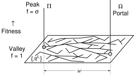
FIG. 1.: Evolution from the peak genotype $\Pi$ to the higher-fitness portal genotype $\Omega$ via low-fitness valley genotypes. The selective advantage of the peak individuals over those in the valley is controlled by the peak height $\sigma$. The portal and peak genotypes are a Hamming (mutational) distance $w$ apart. The domain is the hypercube ${\cal A}^{L}$ of all length-$L$ genotypes.

At time $t=0$ the population starts with all $M$ genotypes located at the peak $\Pi$. We then evolve the population under selection and mutation, as described in the previous section, until the portal genotype $\Omega$ occurs in the population for the first time. (Hence, the portal’s fitness is not relevant.) This defines one evolutionary run. We record the time $t$ at which the portal is discovered. We are interested in the average discovery time $\langle t\rangle$, averaged over an ensemble of such runs. We are particularly interested in the scaling of this barrier crossing time $\langle t\rangle$ as a function of the evolutionary parameters $M$ and $\mu$, as well as the barrier parameters $\sigma$ and $w$.

Let’s briefly review in simple language the evolutionary dynamics before launching into the mathematical analysis. In the parameter regime with $\sigma\gg 1$, where the peak fitness is considerably larger than the valley fitness, and with the mutation rate $\mu$ not too high, the bulk of the population remains at the peak. That is, the population is a quasispecies cloud, centered around the peak genotype $\Pi$ [7]. For such parameter regimes, the barrier is clearly a fitness barrier: the waiting time $\langle t\rangle$ is determined by the time it takes to create a rare sequence of mutant genotypes that crosses the valley between the peak and the portal.

However, as $\sigma\rightarrow 1^{+}$, the fitness barrier transforms into an entropy barrier. For $\sigma=1$ there is no fitness difference between peak and valley genotypes and the entire population simply diffuses through genotype space until the portal is discovered. As we will see below, the entropic regime sets in rather suddenly at a value of $\sigma_{c}$ somewhat above $\sigma=1$. As we show, this transition is the well known error threshold of molecular evolution theory [6]. At $\sigma=\sigma_{c}$, the value of which depends on the population size $M$ and mutation rate $\mu$, the subpopulation on the peak becomes unstable in the sense that all individuals on the peak may be lost through a fluctuation. More precisely, the waiting time for such a fluctuation to occur becomes short in comparison to the fitness-barrier crossing time. When this fluctuation has occurred, there is no longer a restoring “force” that keeps the population concentrated around the peak genotype. The population as a whole diffuses randomly through the valley as if the genotypes were all fitness neutral. While our analysis accurately predicts the barrier crossing times in the fitness-barrier regime, it is notable that beyond the error threshold, in the entropic regime, only order-of-magnitude predictions can be obtained using the current analytical tools.

Calculating the barrier crossing time proceeds in three stages. First, in Sec. III A we determine the population’s quasispecies distribution, defined as the average proportions of individuals located on the peak and in the valley during the metastable state. From this, one directly calculates the average fitness in the population. Second, in Sec. III B we consider the genealogy statistics of individuals in the valley. In the fitness-barrier regime, genealogies in the valley are generally short-lived and are all seeded by mutants of the peak genotype. We approximate the evolution of valley genealogies as a branching process and use this representation to calculate the average barrier crossing time. Third, with this analysis complete, Sec. V E then addresses the transition from the fitness-barrier regime to the entropic one.

A Metastable Quasispecies

Each evolutionary run, the population starts out concentrated at the peak genotype $\Pi$. After a relaxation phase, assumed to be short compared to the barrier crossing time, there will be roughly constant proportions of the population on the peak and in the valley. We now calculate the equilibrium proportion ${P_{\Pi}}$ of peak individuals and the population’s average fitness ${\langle f\rangle}$, after this relaxation phase.

To first approximation, one can neglect back mutations from valley individuals back into the peak genotype. First of all, if $\sigma\gg 1$, selection keeps the bulk of the population on the peak. Additionally, valley individuals produce fewer offspring than peak individuals and they are unlikely—with a probability $1/L$ at most—to move back onto the peak when they mutate. In this regime, the quasispecies distribution is largely the result of a balance between selection expanding the peak population by a factor of $\sigma/{\langle f\rangle}$ and deleterious mutations moving them into the valley with probability $1-(1-\mu)^{L}$. The result is that we have a balance equation for the proportion ${P_{\Pi}}$ of peak individuals given by

$${P_{\Pi}}=\frac{\sigma}{{\langle f\rangle}}(1-\mu)^{L}{P_{\Pi}}~{}.$$ (1)

From this we immediately have that

$${\langle f\rangle}=\sigma(1-\mu)^{L}~{}.$$ (2)

Since we also have that $\langle f\rangle=\sigma P_{\Pi}+1\cdot(1-P_{\Pi})$, we can determine the proportion of peak individuals to be:

$${P_{\Pi}}=\frac{{\langle f\rangle}-1}{\sigma-1}~{}.$$ (3)

For parameters where ${\langle f\rangle}=\sigma(1-\mu)^{L}\gg 1$, Eqs. (2) and (3) give quite accurate predictions for the average fitness and the proportion of individuals on the peak.

In cases where ${\langle f\rangle}$ is close to $1$, a substantial proportion of the population is located in the valley and back mutations from the valley onto the peak must be taken into account. To do this, we introduce the quasispecies Hamming distance distribution $\vec{P}=(P_{0},\ldots,P_{i},\ldots,P_{L})$, where $P_{i}$ is the proportion of individuals located at Hamming distance $i$ from $\Pi$. Thus, $P_{0}={P_{\Pi}}$ indicates the proportion on the peak. Under selection, the distribution $\vec{P}$ changes according to:

$$P^{{\rm sel}}_{i}=\frac{(\sigma-1)\delta_{i0}+1}{{\langle f\rangle}}P_{i}~{},$$ (4)

where $\delta_{ij}=1$, if $i=j$, and $\delta_{ij}=0$, otherwise. We can write this formally as the result of an operator acting on $\vec{P}$:

$$\vec{P}^{{\rm sel}}=\frac{\left({\bf S}\cdot\vec{P}\right)_{i}}{{\langle f\rangle}}~{},$$ (5)

where

$$S_{ij}=\left[(\sigma-1)\delta_{i0}+1\right]\delta_{ij}~{},$$ (6)

defines the selection operator $\bf S$.

Next, we consider the transition probabilities ${\rm M}_{ij}$ that under mutation a genotype at Hamming distance $j$ from the peak moves to a genotype at Hamming distance $i$ from the peak. We have that:

$${\rm M}_{ij} = \sum_{u=0}^{L-j}\sum_{d=0}^{j}\delta_{j+u-d,i}{L-j\choose u}{j\choose d}$$ (8)

$$\times\mu^{u+d}(1-\mu)^{L-u-d}~{}.$$

That is, ${\rm M}_{ij}$ is the sum of the probabilities of all possible ways to mutate $u$ of the $L-j$ bits shared with $\Pi$ and $d$ of the $j$ bits that differ, such that $j+u-d=i$. Equation (8) defines the mutation operator $\bf M$.

We can now introduce the generation operator ${\bf G}={\bf M}\cdot{\bf S}$. The equilibrium quasispecies distribution $\vec{P}$ is a solution of the equation

$$\vec{P}=\frac{{\bf G}\cdot\vec{P}}{{\langle f\rangle}}~{}.$$ (9)

In this way, the quasispecies distribution is given by the principal eigenvector, normalized in probability, of the matrix ${\bf G}$; while the average fitness ${\langle f\rangle}$ is given by ${\bf G}$’s principal eigenvalue. Note that this is conventional quasispecies theory [7], apart from the facts that we have grouped the quasispecies members into Hamming-distance classes and that we consider discrete generations, rather than continuous time.

B Valley Lineages

Under the approximation that back mutations from the valley onto the peak can be neglected, a roughly constant proportion $1-{P_{\Pi}}$ of valley individuals is maintained by a roughly constant influx of mutants from the peak. Every generation, some peak individuals leave mutant offspring in the valley. Additionally, each valley individual leaves on average a fraction $1/{\langle f\rangle}$ offspring in the next generation, as can be seen from Eq. (4). This means that the fraction of valley individuals, for which all of its $t$ ancestors in the previous $t$ generations were valley individuals as well, is only $1/{\langle f\rangle}^{t}$. For ${\langle f\rangle}\gg 1$, this implies in turn that whenever a peak individual seeds a new lineage of valley individuals by leaving a mutant offspring in the valley, this lineage is unlikely to persist for a large number of generations. In other words, lineages composed of valley individuals are short lived.

Intuitively, the idea is that the preferred selection of peak individuals leads to a “surplus” of peak offspring that spills into the valley through mutations. Each mutant offspring of a peak individual forms the root of a relatively small, i.e., short-lived, genealogical tree of valley individuals. The barrier crossing time is determined essentially by the waiting time until one of these genealogical bushes produces a descendant that discovers the portal. These processes are illustrated in Fig. 2.

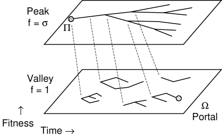
FIG. 2.: Genealogies during fitness-barrier crossing. An example genealogical tree is sketched for peak individuals (above); they have fitness $\sigma$ and are copies of the peak genotype $\Pi$. The valley individuals (below) at lower fitness occur in genealogies that are seeded (dashed lines) from peak individuals. These genealogies are relatively short-lived bushes. Evolution continues until the time at which one of the valley bushes discovers the portal genotype $\Omega$.

We will analyze the evolution of a valley lineage as a branching process [14]. The probability $O_{n}$ that one particular valley individual leaves $n$ offspring in the next generation is given by a binomial distribution. This is well approximated by a Poisson distribution as follows:

$$O_{n} = {M\choose n}\left(\frac{1}{M{\langle f\rangle}}\right)^{n}\left(1-\frac{1}{M{\langle f\rangle}}\right)^{M-n}$$ (10)

$$\approx \frac{1}{n!}\left(\frac{1}{{\langle f\rangle}}\right)^{n}e^{-1/{\langle f\rangle}}~{}.$$ (11)

To a good approximation, we may treat the evolution of each valley lineage as independent of the other valley lineages. Under this approximation, each valley individual independently has a distribution of offspring given by Eq. (10). Of course, under fixed population size, the independence assumption may break down when valley lineages dominate the population.

We now calculate the probability that a valley lineage produces a descendant that discovers the portal $\Omega$ before the lineage goes extinct. Let a valley lineage be founded by an ancestor in the valley that is located at Hamming distance $j$ from $\Omega$. We denote by $\bar{p}_{j}(t)$ the probability that $t$ generations from now, none of this ancestor’s descendants will have discovered the portal. This probability can be determined recursively, in terms of the probabilities $\bar{p}_{i}(t-1)$ as follows,

$$\bar{p}_{j}(t) = O_{0}+O_{1}\sum_{i=1}^{L}\bar{p}_{i}(t-1){\rm M}_{ij}$$ (12)

$$+ O_{2}\sum_{i,k=1}^{L}\bar{p}_{i}(t-1){\rm M}_{ij}\bar{p}_{k}(t-1){\rm M}_{kj}+\ldots~{}.$$ (13)

The first term in the above equation corresponds to the ancestor having no offspring. This, of course, ensures that the portal will not be discovered $t$ generations from now, since leaving zero offspring implies that the genealogy goes extinct immediately. The second term corresponds to the ancestor having one offspring, at Hamming distance $i$ from the portal, that will not give rise to discovery of the portal. That is, since this offspring itself forms the ancestor of a new valley lineage, $\bar{p}_{i}(t-1)$ gives the probability that none of its descendants discovers the portal within the next $t-1$ generations. The third term corresponds to the ancestor having two offspring, one at distance $i$ from the portal and one at distance $k$, neither of which give rise to the discovery of $\Omega$. The higher-order terms in Eq. (12) correspond to the ancestor having $3$, $4$, and more offspring.

Recall that the mutation operator ${\rm M}_{ij}$, as defined in Eq. (8), gave the probability to go from Hamming distance $j$ to distance $i$ from the peak under mutation. ${\rm M}_{ij}$ appears above in Eq. (12) with a different, but equivalent, meaning: ${\rm M}_{ij}$ there gives the probability to go from a Hamming distance $j$ to a distance $i$ from the portal under mutation. This use of ${\rm M}_{ij}$ appears repeatedly in the following.

Using Eq. (10) we can sum the series in Eq. (12), obtaining:

$$\bar{p}_{j}(t)=e^{\left(\left[\bar{\bf p}(t-1)\cdot{\bf M}\right]_{j}-1\right)/{\langle f\rangle}}~{},$$ (14)

where $\bar{p}(t)=(\bar{p}_{1}(t),\bar{p}_{2}(t),\ldots,\bar{p}_{L}(t))$ and the vector notation denotes the sum

$$\left[\bar{p}(t-1)\cdot{\bf M}\right]_{j}=\sum_{i=1}^{L}\bar{p}_{i}(t-1){\rm M}_{ij}~{}.$$ (15)

For ${\langle f\rangle}\geq 1$, a valley genealogy eventually either discovers $\Omega$ or goes extinct; see, for instance, Ref. [14]. Letting $t\rightarrow\infty$ in Eq. (14), we obtain a set of nonlinear equations for the asymptotic probabilities $\bar{p}_{j}$ that a genealogical bush, whose founder started at Hamming distance $j$ from $\Omega$, goes extinct before any of its descendants discovers the portal. These are given by

$$\bar{p}_{j}=e^{\left(\left[\bar{p}\cdot{\bf M}\right]_{j}-1\right)/{\langle f\rangle}}~{}.$$ (16)

Equations (16) appear to be unsolvable in closed analytical form. Their solutions may be numerically approximated in a straightforward manner; for instance, by simply iterating Eq. (14). However, in the regime where $\mu$ is small and ${\langle f\rangle}$ is not too close to $1$, the probabilities $\bar{p}_{i}$ are generally very close to $1$. In this regime, one may expand Eq. (16) to first order around $\bar{p}_{i}=1$. To do this, we introduce the probabilities $\epsilon_{i}=1-\bar{p}_{i}$ that the portal does get discovered by the lineage before it goes extinct. To first order in $\epsilon_{i}$ we obtain from Eq. (16) the equations given by

$$\epsilon_{j}=1-e^{-{\rm M}_{0j}/{\langle f\rangle}}\left(1-\frac{\left[{\bf\epsilon}\cdot{\bf M}\right]_{j}}{{\langle f\rangle}}\right)~{},$$ (17)

where ${\bf\epsilon}=(\epsilon_{1},\ldots,\epsilon_{L})$. These equations can be easily inverted, yielding:

$$\epsilon_{j}=\sum_{i=1}^{L}\left(1-e^{-{\rm M}_{0i}/{\langle f\rangle}}\right)\left({\bf I}-{\bf R}\right)^{-1}_{ij}~{},$$ (18)

where ${\bf I}$ is the identity matrix and the matrix ${\bf R}$ has components

$${\rm R}_{ij}=\frac{{\rm M}_{ij}}{{\langle f\rangle}}e^{-{\rm M}_{0j}/{\langle f\rangle}}~{}.$$ (19)

Note that the indices $i$ and $j$ in the matrices run from $1$ to $L$, corresponding to ancestors at Hamming distances between $1$ and $L$ from the portal. Note also that, by definition, $\epsilon_{0}=1$.

To first order, Eqs. (18) give the probabilities $\epsilon_{j}$ that a valley lineage, founded by an ancestor at a Hamming distance $j$ from $\Omega$, discovers the portal before the lineage goes extinct. Now to calculate the barrier crossing time we just have to determine the number of new valley lineages that are founded per generation.

C Crossing the Fitness Barrier

Every generation, $M$ individuals are selected in proportion to their fitness. Each such selection may lead to the seeding of a new lineage in the valley. The probability $P^{\rm not}$ that a selection will not lead to the founding of a new valley lineage is given by:

$$P^{\rm not}=\frac{1-{P_{\Pi}}}{{\langle f\rangle}}+\frac{\sigma}{{\langle f\rangle}}{P_{\Pi}}(1-\mu)^{L}~{}.$$ (20)

The first term corresponds to selecting a valley individual, that by definition is already on a lineage. The second term corresponds to a peak individual being selected and reproducing without mutation, leaving an offspring on the peak.

The probability $P^{\rm seed}_{j}$ that a new lineage will be seeded in the valley and at a Hamming distance $j$ from $\Omega$ is given by

$$P^{\rm seed}_{j}=\frac{\sigma}{{\langle f\rangle}}{P_{\Pi}}\left[{\rm M}_{jw}-(1-\mu)^{L}\delta_{jw}\right]~{},$$ (21)

where $w$ is the Hamming distance between the peak and the portal. The first factor, $\sigma P_{\Pi}/{\langle f\rangle}$, gives the probability that a peak individual will be selected. The term ${\rm M}_{jw}$ is the probability that under mutation this peak individual moves from Hamming distance $w$ to distance $j$ from the portal. For $j\neq w$ this always corresponds to a new lineage in the valley. For $j=w$, we must discount for the probability that the peak individual did not undergo any mutations at all. This is given by the term $(1-\mu)^{L}\delta_{jw}$.

Putting these together, we find the probability $\bar{P}^{\rm sel}$, that a selection does not seed a lineage leading to the portal, is given by

$$\bar{P}^{\rm sel}=P^{\rm not}+\sum_{j=1}^{L}(1-\epsilon_{j})P^{\rm seed}_{j}.$$ (22)

Using Eqs. (16), (20), and (21) and the identity ${\langle f\rangle}=1+(\sigma-1){P_{\Pi}}$, Eq. (22) can be rewritten as

$$\bar{P}^{\rm sel}=1 + \frac{\sigma({\langle f\rangle}-1)}{(\sigma-1){\langle f\rangle}}$$ (23)

$$\times \left[(1-\mu)^{L}\epsilon_{w}+{\langle f\rangle}\log(1-\epsilon_{w})\right]~{}.$$ (24)

Expanding the logarithm to first order in $\epsilon_{w}$, and using the approximation in Eq. (2) for ${\langle f\rangle}$, we obtain the simple expression

$$\bar{P}^{\rm sel}=1-\epsilon_{w}({\langle f\rangle}-1).$$ (25)

The probability that none of the $M$ selections from the current generation seeds a lineage that discovers the portal is simply $\left(\bar{P}^{\rm sel}\right)^{M}$. By our assumption of a roughly constant quasispecies distribution, this probability is constant. Thus, the expected number $\langle t\rangle$ of generations until a lineage will be seeded that discovers the portal is given by

$$\langle t\rangle=\frac{1}{1-\left(\bar{P}^{\rm sel}\right)^{M}}\approx\frac{1}{M({\langle f\rangle}-1)\epsilon_{w}}~{}.$$ (26)

where $\epsilon_{w}$ is given by Eqs. (18) and (19).

Equation (26) constitutes our theoretical prediction for the average barrier crossing time $\langle t\rangle$ as a function of the population size $M$, the fitness differential $\sigma$ between the peak and the valley, the mutation rate $\mu$, the string length $L$, and the width $w$ of the fitness barrier. To obtain it, we made several approximations. We assumed that $\sigma$ was large enough and $\mu$ small enough such that ${\langle f\rangle}$ was substantially larger than $1$. Under those assumptions, lineages in the valley are short lived, the total number of individuals in the valley will be small with respect to $M$, and the probabilities $\epsilon_{i}$ will be small. This justifies our leading-order expansion for $\langle t\rangle$.

D Additional Time in Valley Bushes

Equation (26) gives the average number $\langle t\rangle$ of generations until a lineage is founded that discovers the portal. The actual average time until the portal is discovered is somewhat longer, since the lineage that finds the portal itself takes a certain average number of generations to discover the portal. Specifically, there is an additional average time, that we denote by $\langle dt\rangle$, between the founding of the first lineage that discovers the portal and the actual discovery of $\Omega$.

We can directly approximate this correction term $\langle dt\rangle$ when the $\epsilon_{i}$ are small. As we will see below, generally $\langle dt\rangle\ll\langle t\rangle$ in the parameter regime where our approximations are valid. This makes the effect of including the correction term $\langle dt\rangle$ rather small in these parameter regimes. However, as we approach the parameter regime where the $\epsilon_{i}$ become large, the average number of generations $\langle t\rangle$ until the founding of the lineage that discovers the portal becomes comparable to the average number of generations $\langle dt\rangle$ that it takes this lineage to actually discover the portal. In this (limited) parameter regime, including the correction term $\langle dt\rangle$ leads to a significant improvement of our theoretical predictions.

Paralleling the development of the Eq. (16), we start by expanding Eq. (14) to first order in $\epsilon_{j}(t)$; the probability that the lineage starting at distance $j$ has discovered the portal by time $t$. We find that

$$\epsilon_{j}(t)=1-e^{-{\rm M}_{0j}/{\langle f\rangle}}\left(1-\frac{\left[{\bf\epsilon}(t-1)\cdot{\bf M}\right]_{j}}{{\langle f\rangle}}\right)~{}.$$ (27)

The expected additional time $\langle dt_{j}\rangle$, given that the lineage started at a Hamming distance $j$ from $\Omega$ and conditioned on the lineage discovering the portal, is formally given by

$$\langle dt_{j}\rangle = \sum_{t=1}^{\infty}t\;\frac{\epsilon_{j}(t)-\epsilon_{j}(t-1)}{\epsilon_{j}}$$ (28)

$$= \sum_{t=0}^{\infty}\frac{\epsilon_{j}-\epsilon_{j}(t)}{\epsilon_{j}}~{},$$ (29)

where the asymptotic $\epsilon_{j}$ is given by Eqs. (18) and (19). Using Eq. (27) and the boundary conditions $\epsilon_{j}(0)=0$, the above sum gives:

$$\langle dt_{j}\rangle=\frac{1}{\epsilon_{j}}\sum_{i=1}^{L}\left(1-e^{-{\rm M}_{0i}/{\langle f\rangle}}\right)\left({\bf I}-{\bf R}\right)^{-2}_{ij},$$ (30)

where the matrix ${\bf R}$ is again defined by Eq. (19).

In order to obtain $\langle dt\rangle$ we have to weigh each of the times $\langle dt_{j}\rangle$ with a factor $c_{j}$ corresponding to the relative proportion of times that a lineage starting at Hamming distance $j$ discovers the portal. That is, averaged over an ensemble of runs, $c_{j}$ is the proportion of times that the portal was discovered by a lineage that started at Hamming distance $j$. The weight $c_{j}$ should be proportional to both the probability $\epsilon_{j}$ and the rate of creating of lineages at Hamming distance $j$ from the portal. We have that

$$c_{j}=\frac{\epsilon_{j}\left({\rm M}_{jw}-(1-\mu)^{L}\delta_{jw}\right)}{\sum_{k}\epsilon_{k}\left({\rm M}_{kw}-(1-\mu)^{L}\delta_{kw}\right)}~{},$$ (31)

$$j=0,1,\ldots,L~{},$$ (32)

where the factors in parentheses are similar to that found in Eq. (21). It should be noted that here the indices run from $0$ to $L$ and not from $1$ to $L$, since the portal may also be discovered by a jump mutation directly from the peak.

Combining Eqs. (30) and (32) and using Eq. (18), we find that the average length of the valley bush that discovers the portal is

$$\langle dt\rangle=\frac{\left[{\bf\epsilon}\cdot\left({\bf I}-{\bf R}\right)\cdot\left({\bf M}-{\bf I}(1-\mu)^{L}\right)\right]_{w}}{\left[{\bf\epsilon}\cdot\left({\bf M}-{\bf I}(1-\mu)^{L}\right)\right]_{w}+{\rm M}_{0w}}~{},$$ (33)

where, again, $\bf\epsilon$ is given by its components in Eqs. (18) and (19). The indices in the vector notation now run from $1$ to $L$.

Adding the correction term $\langle dt\rangle$ to $\langle t\rangle$ as given by Eq. (26) improves our theoretical predictions especially in the regime where the $\epsilon_{i}$ become large. However, we still expect the approximations leading to the above equations for $\langle t\rangle$ and $\langle dt\rangle$ to break down when ${\langle f\rangle}\rightarrow 1^{+}$.

E Theory versus Simulation

We simulated an evolving population using a fitness function consisting of a single barrier, as described in Secs. II and III, for a wide range of parameter settings to quantitatively test our theoretical predictions. Results for several parameter regimes are shown in Fig. 3, where the simulation results are plotted using dashed lines and the theoretical predictions are plotted with solid lines. Each data point on the dashed lines was obtained by averaging over $250$ runs with equal parameter settings. The theoretical predictions are shown as pairs of solid lines, where the lower solid line in each pair shows the predictions from Eq. (26) and the upper solid line shows Eq. (26) plus the correction term of Eq. (33). Note that for most parameter ranges the difference between the two solid lines is so small as to be undetectable.

Figures 3(a) and 3(b) show the average barrier crossing time $\langle t\rangle$ as a function of the logarithm $\log(\sigma)$ of the barrier height. Additionally, both $\langle t\rangle$ and $\log(\sigma)$ are plotted using a logarithmic scale. The shapes of the curves correspond to the dependencies of $\log\langle t\rangle$ on $\log(\log\sigma)$. Portions of curves that are straight lines thus indicate a scaling of the form $\langle t\rangle\propto(\log\sigma)^{s}$, with $s$ the slope of the straight portion. Note that $\langle t\rangle$ ranges over $5$ orders of magnitude, from $10$ to $10^{6}$, in both Figs. 3(a) and 3(b). We see that the theory accurately predicts the simulation results for barrier heights that are not too small.

FIG. 3.: Barrier-crossing times ${\langle t\rangle}$ as a function of barrier height $\sigma$, mutation rate $\mu$, and barrier width $w$, for a variety of parameter settings. The simulation results are plotted using dashed lines. Each point on each dashed line is an estimate of $\langle t\rangle$ averaged over $250$ simulation runs. The theoretical predictions are shown as pairs of solid lines: The lower of each pair gives the theoretical predictions of Eq. (26), while the higher has the additional correction term of Eq. (33) added. Note that, except for the horizontal axis in Fig. (d), all axes use a logarithmic scale. General parameter settings are indicated at the top of each plot, while parameters specific to the different runs are indicated next to the their lines.

In Fig. 3(a) the theory starts deviating from the experimental data around $\log(\sigma)\approx 0.06$ for the upper two curves and around $\log(\sigma)\approx 0.15$ for the lowest. These values of $\sigma$ correspond to selective advantages $\sigma-1$ of the peak of a little over $6$ and $16$ percent, respectively. Notice that the upper two experimental curves are almost horizontal for small values of $\sigma$ up to $\log(\sigma)\approx 0.06$, after which they trend upwards becoming almost linear. As we will show below, it turns out that the location of this crossover is found at the finite-population error threshold that separates the entropy-barrier regime from the fitness-barrier regime. That is, for the parameters $M=250$, $\mu=0.005$, and $L=10$, the critical value $\sigma_{c}$ below which the population dynamics acts effectively as if there were no fitness peak at all occurs around $\log(\sigma_{c})\approx 0.06$. The same phenomenon is observed in the two upper curves of Fig. 3(b): the crossover occurs around $\log(\sigma_{c})\approx 0.05$. Note that the correction terms $\langle dt\rangle$ extend the parameter region over which the theory provides accurate predictions approximately up to the finite-population error threshold.

Above the error threshold, for values of $\sigma$ in the fitness-barrier regime, the curves appear nearly linear. This indicates that the barrier crossing times scale with powers of the logarithm of the barrier height $\sigma$: $\langle t\rangle\propto(\log\sigma)^{s}$, where $s$ is the line’s slope. Thus, the barrier crossing time increases relatively slowly as a function of the barrier height. One further observes that the barrier crossing times are not only longer for wider barriers (larger values of $w$), but that the slopes of the curves are larger as well. That is, for large widths $w$ the barrier crossing time increases faster as a function of $\sigma$ than for low values of $w$.

Figure 3(c) shows the barrier crossing time $\langle t\rangle$ as a function of the mutation rate $\mu$, for three different values of the barrier width $w$ and two different values of the barrier height $\sigma$. The population size is $M=250$ and the genotypes length $L=7$ for all three curves. On the logarithmic scales, the curves again look approximately linear, indicating that the barrier crossing time scales as a power law in the mutation rate $\mu$: $\langle t\rangle\propto\mu^{s}$, where $s$ is the slope. We again see that for wider barriers, the waiting times are both larger and vary more rapidly with $\mu$. The theory predicts the simulation results quite accurately over the entire range. Only for large mutation rates ($\mu\approx 0.01$) do the theoretical predictions with and without the correction term of Eq. (33) differ significantly. In this regime the theoretical and experimental values start to differ slightly as well, although the predictions are still accurate. It is notable in the two lower curve families, with barrier widths $w=2$ and $w=3$, that the correction term $\langle dt\rangle$ improves the theoretical predictions for high mutation rates.

Finally, Fig. 3(d) shows the barrier crossing time ${\langle t\rangle}$ as a function of the barrier width $w$. Only the barrier crossing time ${\langle t\rangle}$ is shown on a logarithmic scale, so that any linear dependence indicates an exponential scaling: ${\langle t\rangle}\propto 10^{sw}$, where $s$ is the slope. Again, the theory accurately predicts the barrier crossing time. The fact that the curves are not linear and bend downwards shows that ${\langle t\rangle}$ grows more slowly than exponential with barrier width; although it still increases rapidly as a function of $w$. In fact, we chose large values of the mutation rate $\mu$ in these plots ($\mu=0.01$ and $\mu=0.015$) to ensure that the barrier crossing time is still in a reasonably bounded range up to large barrier widths. For smaller mutation rates, the barrier crossing times become so large as to make it impossible to perform an adequate number of simulation runs. For the case $w=1$, the correction term $\langle dt\rangle$ leads to an overestimation of ${\langle t\rangle}$. Note, however, that for $w=1$ there is effectively no fitness barrier; the portal is a mutant neighbor of the peak genotype and so valley bushes are essentially nonexistent.

In summary, Figs. 3(a)-(d) show that the theoretical predictions of Eq. (26), possibly including the correction term of Eq. (33), accurately predict the average barrier crossing times estimated over a wide range of parameters from simulations of an evolving population. The theory breaks down, as expected, when the barrier height $\sigma$ becomes small ($\sigma\approx 1$) and this is illustrated on the left-hand sides of Figs. 3(a) and 3(b). In this low-$\sigma$ regime, which sets in suddenly as a function of $\sigma$, ${\langle t\rangle}$ becomes almost independent of $\sigma$. Roughly speaking, the selection pressure is too small to keep the population concentrated around the peak, and the population randomly diffuses through the valley until it discovers the portal. In this regime, the barrier is in effect not a fitness barrier, but an entropy barrier.

In Sec. IV we will analyze the location of the finite-population error threshold that separates the fitness and entropy barrier regimes and discuss the entropy-barrier crossing population dynamics. In the next subsection, though, we first discuss the scaling of the fitness-barrier crossing time ${\langle t\rangle}$ with the different parameters $\sigma$, $w$, $\mu$, and $M$.

F Scaling of the Barrier Crossing Time

In Fig. 3 we saw, by varying one parameter at a time, that the barrier crossing time scaled as a power law in the logarithm of the barrier height $\log(\sigma)$, as a power law in mutation rate $\mu$, and somewhat slower than exponential in the barrier width $w$. Analytically extracting these scalings from Eq. (26) is quite challenging and incomplete at this time. Empirically, though, we found that the barrier crossing time can be fit quite accurately, in the regime where $\sigma$ is not too small (above the error threshold), to a scaling function with the following form

$$\langle t\rangle\propto\frac{1}{w!M\mu} \left(\frac{\log(\sigma)}{\mu}\right)^{w-1}$$ (34)

$$\times \left[\log(\sigma)\right]^{-\gamma-\delta\log(\mu)}~{},$$ (35)

where $\gamma$ and $\delta$ are (constant) scaling exponents. For both the genotype lengths ($L=7$ and $L=10$) for which we have detailed data, we found that $\gamma\approx 0.75$ and $\delta\approx 0.1$.

This empirical scaling law confirms that, in fact, the barrier crossing time ${\langle t\rangle}$ scales as a power law in both $\log(\sigma)$ and $\mu$. We see, in particular, that the dependence on the mutation rate $\mu$ scales roughly inversely with $\mu^{w}$ and the dependence on $\log(\sigma)$ scales roughly as $\left[\log(\sigma)\right]^{w-2}$. Furthermore, we see that ${\langle t\rangle}$ scales as $e^{cw}/w!$, with $c$ a constant, when only the barrier width $w$ is varied. The scaling with $w$ is thus by far the most rapid and therefore dominant scaling. That is, widening the barrier increases the waiting time ${\langle t\rangle}$ much more than increasing the height of the barrier or decreasing the mutation rate.

These empirically observed scaling behaviors can be elucidated using a simple analytical argument. To this end we employ several simplifications. First, we assume that the major contributions to the probability of barrier crossing come from terms with the minimal number of mutations. That is, for barriers of width $w$, at least $w$ mutations must occur in a peak individual in order to discover the portal. Thus, we assume that contributions from “paths” between peak and portal that involve more than $w$ mutations are negligible. This for instance implies that we neglect the contributions from lineages founded at Hamming distances $w$ through $L$ from $\Omega$. Furthermore, we assume that valley lineages are unlikely to be founded more than $1$ mutation away from the peak. Putting these together, the dominant contribution to the barrier crossing probability comes from lineages that are founded at a Hamming distance $w-1$ from the portal. Note that if we set $P_{\Pi}=1$ for simplicity, each generation approximately

$$\frac{w\mu M}{1-\mu}$$ (36)

such lineages are founded.

We will now estimate the probability that a lineage, starting at Hamming distance $w-1$ from the portal, discovers the portal exactly $t$ generations after its founding. We approximate the valley genealogies by assuming that each valley individual can only have zero or one offspring each generation. This implies that a valley lineage consists of a single line of individuals; i.e., lineages do not branch. The probability that such a lineage persists for at least $t$ time steps is $1/{\langle f\rangle}^{t}$. At $t=0$, the lineage has $w-1$ bits set incorrectly, and $L-w+1$ bits set correctly. In order for the lineage to discover the portal exactly at time $t$, it will have to mutate its bits such that, at time $t$ and for the first time, the $w-1$ “incorrect” bits will all have been flipped to the correct state and all the $L-w+1$ correct bits are left undisturbed. Thus, between time $0$ and $t$, the $w-1$ incorrect bits have to be mutated exactly once, while the correct bits have been undisturbed. Since we are calculating the probability for the portal to be discovered exactly at time $t$, one of the $w-1$ bits has to flip at time $t$, while the other $w-2$ might flip at any prior time. This gives $(w-1)\>t^{w-2}$ possibilities for contributing flips. All other bits have to remain unflipped for all time steps.

Thus, the probability $P^{{\rm find}}_{t}$ that a lineage finds the portal exactly at time $t$ is approximately given by:

$$P^{{\rm find}}_{t} = (w-1)\>t^{w-2}$$ (37)

$$\times \mu^{w-1}(1-\mu)^{Lt-w+1}\left(\frac{1}{{\langle f\rangle}}\right)^{t}~{},$$ (38)

where the last factor gives the probability that the lineage survives until time $t$. Using Eq. (2) and summing Eq. (38) over $t$ we find:

$$P^{{\rm find}} = \sum_{t=0}^{\infty}P^{\rm find}_{t}$$ (39)

$$= (w-1)\left(\frac{\mu}{1-\mu}\right)^{w-1}\sum_{t=0}^{\infty}t^{w-2}\left(\frac{1}{\sigma}\right)^{t}$$ (40)

$$= (w-1)\left(\frac{\mu}{1-\mu}\right)^{w-1}{\rm Li}_{2-w}\left(\frac{1}{\sigma}\right)~{},$$ (41)

where ${\rm Li}_{n}(x)$ is the poly-logarithm function: essentially defined by the sum in the second line above. It is more insightful to approximate the sum with an integral. We then obtain

$$P^{{\rm find}} = \left(\frac{\mu}{1-\mu}\right)^{w-1}\int_{0}^{\infty}(w-1)\>t^{w-2}e^{-\log(\sigma)t}dt$$ (42)

$$= (w-1)!\left(\frac{\mu}{\log(\sigma)(1-\mu)}\right)^{w-1}~{}.$$ (43)

Recall that the rate at which lineages at Hamming distance $w-1$ are being created is $w\mu M/(1-\mu)$. Using this and noting that the barrier crossing time is inversely proportional to $P^{\rm find}$, we obtain a scaling of the form

$$\langle t\rangle\propto\frac{1}{w!M\mu}\left(\frac{\log(\sigma)}{\mu}\right)^{w-1}~{},$$ (44)

where we have neglected the factor $(1-\mu)^{w}\approx 1$. The scaling relation of Eq. (44) recovers most of the empirically determined scaling behavior in Eq. (34).

The dominant scaling with $\mu$ and $\log(\sigma)$ can be understood as follows. The average time that a lineage spends in the valley before going extinct is roughly $1/\log(\sigma)$. Thus, $\mu/\log(\sigma)$ gives the average number of mutations that a lineage in the valley undergoes before it goes extinct. Since this number is generally much smaller than $1$, it can be interpreted as the probability of having a single mutation in a valley lineage. The probability of having $w-1$ mutations is then of course $(\mu/\log(\sigma))^{w-1}$. There is an additional factor $1/\mu$ from the rate at which valley lineages are being created at Hamming distance $w-1$. Ref. [31] also argues, along somewhat different lines, that the barrier crossing time should have a power-law dependence on mutation rate: $\langle t\rangle\propto\mu^{-w}$.

The correction factors—those with scaling exponents $\gamma$ and $\delta$ in Eq. (34)— probably arise from the fact that lineages are not simple unbranching lines of descendants, as we have assumed, but are more complicated tree-like genealogies.

The factor $w!$ in Eq. (44) counts the number of distinct paths of minimal length between the peak and the portal. Curiously, it appears from the scaling formulas that when $w$ gets very large, the barrier crossing time starts to decrease again. Applying Stirling’s approximation to the factorial function in Eq. (44) indicates that ${\langle t\rangle}$ has a maximum around $w\mu=\log(\sigma)$. Although this may initially seem strange, it does make sense, since as we will now argue, fitness barriers for which $w\mu>\log(\sigma)$ do not exist.

If there are $w!$ independent paths between peak and portal, this implies that there are $w$ independent directions from the peak into the valley. In other words, at least $w$ bits of the peak genotype can undergo deleterious mutations. As we will see in Sec. IV below, the error threshold at which peak individuals becomes unstable in the population occurs near

$$\sigma(1-\mu)^{L}=1~{}.$$ (45)

To first order in $\mu$, this is equivalent to $\log(\sigma)=L\mu$. That is, if $L\mu>\log(\sigma)$, peak individuals will be lost from the population, and the population will start diffusing randomly through genotype space. Obviously, the genotype length has to be longer than the barrier width $L>w$. Therefore, $w\mu>\log(\sigma)$ implies that the genotype length $L$ is so large that it is impossible to stabilize the peak individuals. In other words, fitness barriers with $w\mu>\log(\sigma)$ simply do not exist.

Finally, it should be noted that as $\log(\sigma)\rightarrow\infty$, the barrier crossing time goes to a finite asymptote and not to infinity. Since valley lineages have probability zero to reproduce in this limit, the asymptotic barrier crossing time is given by the (finite) waiting time for a “long jump” in which a peak individual undergoes $w$ mutations at once.

The main consequence of the scaling relations just derived, is that if the population is located on a fitness “plateau” in genotype space, surrounded by different valleys on all sides, then it will most likely escape from the plateau via the valley with the smallest width and not via the valley path with the smallest depth. One concludes that high barriers can be passed relatively easily, as long as they are narrow; while wide barriers take a very long time to cross, even if they are shallow.

We should emphasize that this situation is very different from the scaling of barrier crossing times generally encountered in physics or, for that matter, in evolutionary models that literally interpret the “landscape” metaphor as leading to stochastic gradient dynamics on a fitness “potential”. In these settings, the system’s state space has an energy function defined on it that acts as a potential field. In the absence of any noise, the system is assumed to follow the gradient (downward) of the energy “landscape”. In the presence of noise, the system can deviate from its gradient path, but movement against the gradient is unlikely in proportion to its deviation from the local gradient. The barrier crossing times then depend mainly on the barrier height, and they scale exponentially with this barrier height [12].

For example, imagine an energy barrier that consists of a steep slope upwards, followed by a long plateau and then a steep slope leading downward on the other side. The initial steep ascent from the valley onto the plateau is very unlikely since it involves moving against a steep gradient. However, after this unlikely step has been established, the system can cross the long plateau to the other side relatively easily, since it does not involve moving against an energy gradient. Thus, the width of the energy barrier is almost immaterial, while the barrier height is the defining impediment, since it determines the extent to which movement against the gradient must occur.

The situation is entirely different for fitness “landscapes” in which an evolving population moves. For an evolving population, making a large jump in fitness is not unlikely at all. One mutation in one individual can do the trick. However, since some individuals remain at the peak, the individuals in the valley are continuously in competition with these higher-fitness peak individuals. An absolute fitness scale is set by these peak individuals. It is therefore survival at low fitness—compared to the most-fit individuals in the population—for an extended period of time that is unlikely. And this is why the time it takes to move across the plateau is the key parameter—which, of course, is controlled by the barrier width.

The preceding discussion should make it clear, once again, that this analogy—between a population evolving over a fitness “landscape” and a physical system moving over its energy “landscape” in state space—is problematic: at best it may lead one to the wrong intuitions; at worst the basic physical results simply do not describe evolutionary behavior.

IV The Entropy Barrier Regime

Figures 3(a) and 3(b) showed that below a critical barrier height $\sigma_{c}$, where the dashed lines began to run horizontally, the barrier crossing time became effectively independent of $\sigma$. We also saw that the theory breaks down for $\sigma<\sigma_{c}$. In this regime, all peak individuals are quickly lost and the population diffuses through the valley until the portal is discovered. The theoretical calculations, in contrast, assumed the population was located at the peak and that short lineages were continuously spawned in the valley. It is no surprise then that the predictions break down in this regime. Since the population dynamics is dominated by diffusing through the valley’s fitness-neutral volume, we refer to this as the entropy-barrier regime. Before discussing the barrier crossing times in this entropic regime, we first estimate the error threshold’s location $\sigma_{c}$ as a function of $\mu$, $M$, and $L$.

A Error Thresholds

As a first, population-size independent approximation one might guess that the error threshold occurs when the average number of peak-offspring produced by a single peak individual in a population of valley individuals is $1$. From Eq. (2) this leads to an estimated critical barrier height $\sigma_{c}$ of

$$\sigma_{c}=(1-\mu)^{-L}~{}.$$ (46)

This equation is the standard error-threshold result in molecular quasispecies theory [6, 7]. For the parameters $L=10$ and $\mu=0.005$ of Fig. 3(a), this leads to $\log(\sigma_{c})\approx 0.05$, or $\sigma_{c}\approx 1.05$. As seen from the figure, though, the entropic regime extends to somewhat higher peak fitness; as far as $\log(\sigma)\approx 0.06$. This deviation is due to finite-population sampling effects and to neglecting back mutations, which become important as the error threshold is approached.

For finite populations, the error threshold can be defined most naturally as those parameter values for which the mean proportion ${P_{\Pi}}$ of peak individuals equals the variance, due to finite population fluctuations, in ${P_{\Pi}}$. That is, the criterion for reaching the error threshold is

$$({P_{\Pi}})^{2}={\rm Var}({P_{\Pi}})~{}.$$ (47)

The intuition behind this definition is as follows: Since the proportion of peak individuals fluctuates, eventually a large fluctuation will occur that leads to the loss of all peak individuals. As was shown in Ref. [30], however, the waiting time for such a destabilization to occur increases exponentially with the ratio $({P_{\Pi}})^{2}/{\rm Var}({P_{\Pi}})$. Only when $({P_{\Pi}})^{2}<{\rm Var}({P_{\Pi}})$ do such destabilizations occur relatively frequently. For $({P_{\Pi}})^{2}>{\rm Var}({P_{\Pi}})$ the fluctuations are small enough so that the proportion of peak individuals typically does not vanish. Therefore, it is natural to use Eq. (47) to delineate the regimes with “unstable” and “stable” peak populations and so to distinguish between the fitness-barrier and entropy-barrier regimes in the population dynamics.

Finite-population error thresholds may also be defined in alternative ways; cf. Ref. [24]. Typically, one finds that, although the conceptual motivations differ, the quantitative parameter values for which the different error thresholds occur are quite similar.

The variance ${\rm Var}({P_{\Pi}})$ can be most easily calculated using diffusion-equation methods. For an introduction to these techniques in the context of mathematical population genetics, see for instance Ref. [18]. To begin, we assume that, due to sampling fluctuations, at some particular time $t$ the actual proportion of peak individuals is not ${P_{\Pi}}$ but instead is $P(t)={P_{\Pi}}+x(t)$. That is, the proportion $P(t)$ of individuals on the peak deviates $x(t)$ from its equilibrium value ${P_{\Pi}}$. We focus on the dynamics of the deviation $x(t)$. At the next generation, the expected deviation $\langle x(t+1)\rangle$ is

$$\langle x(t+1)\rangle=\frac{x(t)}{{\langle f\rangle}}~{}.$$ (48)

Thus, the expected change $\langle\delta x\rangle$ in the deviation is given by

$$\langle\delta x\rangle=\frac{1-{\langle f\rangle}}{{\langle f\rangle}}\>x\equiv-\gamma\>x~{},$$ (49)

where we have defined $\gamma$ by the last equality. $\gamma$ measures the average rate at which fluctuations around the quasispecies equilibrium distribution are damped. The second moment $\langle\left(\delta x\right)^{2}\rangle$ of the change $\delta x$ is approximately given by the variance of the binomial-sampling distribution. One finds that

$$\langle\left(\delta x\right)^{2}\rangle=\frac{1}{M}\left({P_{\Pi}}+\frac{x}{{\langle f\rangle}}\right)\left(1-{P_{\Pi}}-\frac{x}{{\langle f\rangle}}\right).$$ (50)

A Fokker-Planck diffusion equation approximation determines the temporal evolution of distribution ${\rm Pr}(x,t)$ of $x(t)$ via

$$\frac{\partial}{\partial t}{\rm Pr}(x,t)= - \frac{\partial}{\partial x}\langle\delta x\rangle{\rm Pr}(x,t)$$ (51)

$$+ \frac{1}{2}\frac{\partial^{2}}{\partial x^{2}}\langle(\delta x)^{2}\rangle{\rm Pr}(x,t)~{},$$ (52)

where $\langle\delta x\rangle$ from Eq. (49) gives the drift term and $\langle(\delta x)^{2}\rangle$ from Eq. (50) the diffusion term. Solving for the limit distribution ${\rm Pr}(x)$ for $x$ yields

$${\rm Pr}(x) = C\left({P_{\Pi}}+\frac{x}{{\langle f\rangle}}\right)^{2M{\langle f\rangle}({\langle f\rangle}-1){P_{\Pi}}}$$ (53)

$$\times \left(1-{P_{\Pi}}-\frac{x}{{\langle f\rangle}}\right)^{2M{\langle f\rangle}({\langle f\rangle}-1)(1-{P_{\Pi}})}~{}.$$ (54)

Here $C$ is a normalization constant that ensures ${\rm Pr}(x)$ is normalized on the interval $x\in[-{P_{\Pi}},1-{P_{\Pi}}]$. If we expand the fluctuations to second-order around $x=0$, the distribution becomes a Gaussian given by

$${\rm Pr}(x)=\tilde{C}e^{-\frac{M\gamma}{{P_{\Pi}}(1-{P_{\Pi}})}x^{2}},$$ (55)

where $\tilde{C}$ is again a normalization constant. From this distribution of fluctuations one directly reads off the variance ${\rm Var}({P_{\Pi}})$, finding that

$${\rm Var}({P_{\Pi}}) = \frac{{P_{\Pi}}(1-{P_{\Pi}})}{2M\gamma}$$ (56)

$$= \frac{{\langle f\rangle}\left(\sigma-{\langle f\rangle}\right)}{2M(\sigma-1)^{2}}~{},$$ (57)

where we used Eqs. (3) and (49) to arrive at the last line.

As noted before, we define the finite-population error threshold by those parameter values for which $({P_{\Pi}})^{2}={\rm Var}({P_{\Pi}})$. Using Eq. (57) leads to the error-threshold parameter constraints given by

$$\frac{2M({\langle f\rangle}-1)^{2}}{{\langle f\rangle}(\sigma-{\langle f\rangle})}=1.$$ (58)

If we substitute the parameter values $\mu=0.005$, $M=250$, and $L=10$ of Fig. 3(a) and use Eq. (2) for ${\langle f\rangle}$, we find the error threshold at $\log(\sigma_{c})\approx 0.059$. This agrees quite well with the location at which the experimental curves start bending upwards with increasing peak height.

B The “Landscape” Regime

As we have pointed out previously, the scaling relations derived in Sec. III F contrast strongly with those based on “landscape” models in which the population as a whole diffuses through the fitness landscape [20, 22]. For those models, the barrier crossing time scales exponentially with population size and barrier height. It turns out that this scaling behavior—appropriate to the “landscape” regime—can be reconciled with the scaling formulas derived in Sec. III F by closer inspection of Eq. (58).

As noted above, the average destabilization time for a fluctuation to occur that makes all peak individuals disappear from the population scales exponentially in the ratio ${\rm Var}(P_{\Pi})/(P_{\Pi})^{2}$ given by Eq. (58). Thus, Eq. (58) shows that this destabilization time increases exponentially with population size. For cases where $\langle f\rangle\gg 1$ and for reasonable population sizes, the destabilization time is so large that the barrier crossing time is determined by how long it takes a rare mutant to cross the fitness valley.

Close to the finite-population error-threshold ($\langle f\rangle\approx 1$), however, it might be the case that the time to create such a rare sequence of mutants is long in comparison to the destabilization time. In this situation, the barrier crossing time is essentially given by the destabilization time: As soon as all peak individuals are lost, the population diffuses through the valley and quickly discovers the portal. Thus, in the very restricted “landscape” parameter regime just around the error-threshold, the barrier crossing time is determined by the destabilization time and does scale exponentially with population size and barrier height.

Beyond the error threshold—that is, for smaller populations, larger mutation rates, smaller barrier heights, or longer genotypes—the peak readily becomes unoccupied. In this regime, the barrier crossing time becomes almost independent of barrier height $\sigma$. The barrier to be crossed is then no longer a fitness barrier. Instead, it has become an entropy barrier. The population must search through almost all of the valley until the portal is discovered. Thus, only for parameters near the boundary between the fitness and entropic regime does the barrier crossing time scale in accordance with the “landscape” models.

C Time Scales in the Entropic Regime

The population dynamics in the entropic regime beyond the error threshold is modeled most directly by considering an entirely flat (constant) fitness function; in particular, one in which all genotypes have fitness $1$ and containing a single portal $\Omega$. The population starts out concentrated on a genotype at Hamming distance $w$ from $\Omega$ and evolves under selection and mutation until the portal genotype is discovered for the first time. Denote this average entropy-barrier crossing time by $\tau$.

The calculation of the entropy-barrier crossing time appears less analytically tractable than the calculation of the fitness-barrier crossing time. The main difficulty arises from the sampling of individuals at each generation, combined with the global constraint of a fixed population size. Due to this sampling dynamics, subtle genetic correlations emerge between the individuals. Although some of the aspects of the correlation statistics have been derived analytically [5], the entropy-barrier crossing time $\tau$ depends in a complicated, and not yet well understood, way on these correlations. We will discuss the difficulties with calculating entropic barrier crossing time by deriving several simple approximations and discussing why they fail to provide accurate quantitative predictions.

First, one can approximate the neutral evolution just defined by assuming that each individual in the population has exactly one offspring. In this case, the population effectively consists of $M$ independent random walkers that diffuse through genotype space. Since each individual has only one offspring one can identify its genealogy with a single evolving genotype that mutates each bit with probability $\mu$ at each generation. Since $\mu L\ll 1$ in general, this genotype effectively performs a random walk in the hypercube, where random walk steps are made at a rate of one step per $1/(L\mu)$ generations on average.

The average time $\tau_{1}$ a single random walker takes to discover $\Omega$ is given by:

$$\tau_{1}=\sum_{i=1}^{L}\left({\bf I}-{\bf M}\right)^{-1}_{iw}~{},$$ (59)

where the matrix indices run from Hamming distance $1$ through $L$. $\tau_{1}$ determines an upper bound for the entire population’s barrier crossing time. For parameter settings in the fixation regime, where $ML\mu\ll 1$, sampling fluctuations cause the population to converge onto $M$ copies of a single genotype. As is well known from the theory of neutral evolution [19], this set of identical genotypes performs a random walk through the genotype space at the same rate as a single individual. Thus, in this limit, $\tau_{1}$ gives a reasonable prediction for the entropy-barrier crossing time. However, for Fig. 3(a)’s parameter settings ($M=250$, $\mu=0.005$, and $L=10$) that give $ML\mu=12.5$, we find that $\tau_{1}\approx 23000$, almost independent of valley width $w$. Of course, this grossly overestimates the observed barrier crossing times, which vary from ${\langle t\rangle}\approx 25$ for $w=2$ to ${\langle t\rangle}\approx 227$ for $w=4$.

For $M$ independent random walkers, one might simply assume that the waiting time would be roughly a factor $M$ slower, i.e. $\tau_{M}=\tau_{1}/M$. Unfortunately, this leads to $\tau_{M}\approx 93$ which overestimates the observed time for $w=2$ and underestimates ${\langle t\rangle}$ for $w=4$.

The precise probability $\bar{p}_{w}(t)$, that none of $M$ independent random walkers starting at a Hamming distance $w$ have found the portal by time $t$, is given by:

$$\bar{p}_{w}(t)=\left(\sum_{i=1}^{L}{\rm M}^{t}_{iw}\right)^{M}~{}.$$ (60)

From this, one estimates the average entropy-barrier crossing time $\tau$ to be:

$$\tau_{M} = \sum_{t=1}^{\infty}t\left[\bar{p}_{w}(t-1)-\bar{p}_{w}(t)\right]$$ (61)

$$= \sum_{t=0}^{\infty}\bar{p}_{w}(t)~{}.$$ (62)

For Fig. 3(a)’s parameters, Eq. (62) gives $\tau\approx 15$, $58$, and $117$ for barrier widths $w=2$, $3$, and $4$, respectively. These values underestimate each observed waiting time by almost a factor of $2$. Apparently, sampling fluctuations cause the population to explore the genotype space less rapidly than independent random walkers do. As already noted above, the reason for this is that sampling convergence leads different individuals to evolve genetic correlations to some degree.

One way to think about this is to investigate genealogies. Ref. [5] showed that the probability ${\rm Pr}(t)$ for two randomly chosen individuals in the current population to have had a common ancestor less than $t$ generations ago is approximately given by

$${\rm Pr}(t)\approx 1-e^{-t/M}~{}.$$ (63)

This means that, on average, a pair of individuals has only undergone $ML\mu$ mutations each since the time $t\approx M$ they descended from a common ancestor. When $M\mu$ is not much larger than $1$, this implies that two individuals are more strongly correlated genetically than random genotypes. Due to this, it is easy to see, at least qualitatively, that the entropy-barrier crossing time is longer than that predicted for independent random walkers. The correlation, or clustering, of individuals in genotype space leads the population to explore the valley’s neutral volume at a slower rate. Thus, the predictions obtained by assuming $M$ random walkers, as given by Eqs. (60) and (62), are lower bounds to the actual waiting times.

It turns out that the upper (Eq. (59)) and lower (Eq. (62)) estimates do not tightly bound the actual waiting times ${\langle t\rangle}$. They may differ by several orders of magnitude. Fortunately, the lower bound obtained from Eqs. (60) and (62) typically produces reasonable order-of-magnitude estimates for parameter regimes in which $ML\mu>1$. This order-of-magnitude estimate gives the following scaling relation for the entropy-barrier crossing time

$$\tau\approx\frac{2^{L}}{ML\mu}~{}.$$ (64)

D Anomalous Scaling

The order-of-magnitude estimate given by Eq. (64) predicts that the the entropy-barrier crossing time $\tau$ scales inversely with both $\mu$ and $M$. This scaling is, of course, exactly one’s intuitive expectation: the rate at which the genotype space is explored is proportional to both mutation rate $\mu$ and population size $M$. $M$ individuals cover $M$ times as much genotypic “ground” as one individual. Individuals that “move” twice as fast, cover twice as much ground as well. And so, the waiting time should be inversely proportional to both $M$ and $\mu$, which set the exploration rate.

In light of this, it is interesting that data from simulations shows that the entropy-barrier crossing time $\tau$ scales as a power law in both $\mu$ and $M$, but not with exponents equal to $-1$, as the preceding simple argument suggests. To be clearer on this point, Fig. 4 illustrates the observed scaling behavior of the entropy-barrier crossing time as a function of $M$ and $\mu$.

The solid lines plot the data obtained from simulations while the dashed lines show scaling (power-law) functions that were fitted to the experimental data. All axes use logarithmic scales. All simulations were performed with genotypes of length $L=10$ bits. In all of the runs, at time $t=0$ all individuals start at Hamming distance $w=5$ from the portal. Figure 4(a) shows $\tau$’s dependence on $M$ for three different values of $\mu$. The approximately straight lines show that the entropy-barrier crossing time depends roughly as a power law on the population size $M$:

$$\tau\propto\frac{1}{M^{\alpha}}~{}.$$ (65)

Of course, the scaling exponent $\alpha$ may itself depend on $\mu$.

Similarly, Fig. 4(b) shows the dependence of $\tau$ on $\mu$ for two different values of $M$. In this case too, the curves appear well approximated by a straight line, indicating that for fixed $M$ the dependence on $\mu$ is roughly given by

$$\tau\propto\frac{1}{\mu^{\beta}}~{},$$ (66)

where $\beta$ may again depend on the population size $M$. In Table I the exponents of the estimated dashed lines in Figs. 4(a) and 4(b) are given, along with their estimated errors.

$\mu$	$0.002$	$0.005$	$0.008$
$\alpha$	$0.740\pm 0.01$	$0.744\pm 0.02$	$0.761\pm 0.03$
M	$50$	$250$
$\beta$	$1.292\pm 0.008$	$1.365\pm 0.014$

TABLE I.: Estimated exponents $\alpha$ and $\beta$ as defined by Eqs. (65) and (66).

FIG. 4.: Entropy-barrier crossing time $\tau$ as a function of population size $M$ and mutation rate $\mu$. The solid lines are data obtained from simulations, while the dashed lines show the estimated scaling functions. All experiments were done with genotypes of length $L=10$ and a barrier width of $w=5$. All axes are shown on logarithmic scales. In Fig. (a) $\tau$ is shown as a function of population size $M$ for three values of the mutation rate $\mu$. In Fig. (b) $\tau$ is shown as a function of the mutation rate $\mu$ for two values of population size $M$. The approximately straight lines show that $\tau$ scales as a power law in $M$ when $\mu$ is kept constant and, vice versa, as a power law in $\mu$ when $M$ is kept constant. Table I lists the estimated exponents for the power laws. These were used to plot the dashed lines.

The values of the exponents $\alpha$ for different $\mu$ and $\beta$ for different $M$ are very close to each other; $\alpha\approx 3/4$ and $\beta\approx 4/3$. It is clear, however, that they are not constants: $\alpha$ does depend on $\mu$ and $\beta$ on $M$. Note that the estimates for $\alpha$ are all below $1$, while those for $\beta$ are above $1$. Thus, doubling the population size decreases $\tau$ by less than a factor of two, while doubling the mutation rate decreases $\tau$ with more than a factor of two. Intuitively, what is happening is that, due to the clustering in the population, doubling the population size does not lead to a doubling of the exploration rate. That is, some of the “added” members in the larger population will simply occur at genotypes where other members of the population are already located. Thus, they do not contribute to additional novel exploration. In contrast, doubling the mutation rate not only doubles the rate of movement (diffusion) of individuals in the population, it additionally decreases the clustering and so reduces genetic correlations. Due to the combination of these two effects, the entropy-barrier crossing time decreases more than a factor two.

Of course, one would like to predict these anomalous exponents. In principle, they should be calculable from knowledge of the clustering structure of the population at different values of $M$ and $\mu$. For example, if we view the population as a blob or collection of blobs in genotype space, one would like to know how many distinct genotypes, on average, are neighboring one or more individuals of the population. Roughly speaking, we would like to know the average “surface area” of the population in genotype space. Knowledge of this statistic would then supply us with the average probability that a mutation leads to a genotype not currently present in the population. This, in turn, quantifies the population’s rate of exploring novel genotypes, while taking into account genetic correlations. Although several statistics of these genotype blobs were calculated in Ref. [5], we have at present not been able to adapt these results to infer the necessary type of statistics just outlined. The analytical prediction of the scaling exponents $\alpha$ and $\beta$ thus awaits further progress. For the present, we will use our order-of-magnitude estimate in Eq. (64) to compare the entropy-barrier crossing time with the fitness-barrier crossing times.

In summary, we analyzed the fitness- and entropy-barrier crossing times for the simplest (single peak) landscapes in which both types of barrier occur. Our results are summarized by the scaling relations of Eqs. (34) and (64). In the following sections, we apply the preceding analysis to more complicated fitness functions that contain multiple fitness and entropy barriers.

V Traversing Complex Fitness Functions

Up to this point, to make analytical progress we focused on fitness functions that were intentionally simple: a single portal and a single peak in genotype space. Despite this, the analysis of barrier crossing times just developed can be extended with relative ease to more complicated evolutionary processes. To illustrate this extension of the theory, we now introduce a class of more complicated fitness functions that contain multiple fitness and entropy barriers of tunable width and height. That is, in this class of fitness functions, the population may have to cross both a fitness and entropy barrier to escape from its metastable state. Since the relative sizes of both these types of barriers can be tuned, we can explicitly compare the time scales for crossing fitness and entropy barriers within the same evolutionary process.

A The Royal Staircase with Ditches

The class of fitness functions which we call the Royal Staircase with Ditches is closely related to the Royal Staircase and Royal Road fitness functions that we have analyzed previously [4, 27, 28, 29, 30]. Those fitness functions did not contain fitness barriers but instead consisted of a series of entropy barriers. The function class of Royal Staircases with Ditches generalizes these fitness functions and is defined as follows:

• Genotypes consist of bit sequences of length $L$, interpreted as $N$ blocks of $K$ bits each: $L=NK$.

• The blocks are ordered, not in the sense that they correspond to particular positions in the genotype, but only in the sense that they are indexed $1$ through $N$. Note that since our evolutionary process does not include recombination, the population dynamics is invariant under arbitrary permutations of a genotype’s bits. For convenience, we order the blocks from left to right in the genotypes. That is, bits $1$ through $K$ belong to the first block, bits $K+1$ through $2K$ belong to the second block, and so on.

• The $2^{K}$ possible configurations of the $K$-bit blocks each are divided into three classes.

  1. Type-$A$ blocks consist of a configuration with $K$ ones:

     $$A=\underbrace{111\cdots 111}_{K}~{}.$$ (67)

  2. Type-$B$ blocks consist of a configuration with $K-w$ ones and $w$ zeros:

     $$B=\underbrace{111\cdots 111}_{K-w}\overbrace{000\cdots 000}^{w}~{}.$$ (68)

     As will become clear, the parameter $w$ controls the width of the barriers.

  3. All other $2^{K}-2$ configurations are denoted as Type-$*$ blocks.

• A genotype $s$ with blocks $1$ through $n-2$ of type $B$ and block $n-1$ of type $A$ receives fitness $f(s)=n$. These genotypes have the structure:

  $$\underbrace{BB\cdots BB}_{n-2}A\overbrace{**\cdots**}^{N-n+1}~{}.$$ (69)

  Note that the configurations of blocks $n$ through $N$ are immaterial (denoted $*$) when the first $n-1$ blocks occur in the above genotype configuration.

• Genotypes $s$ with blocks $1$ through $n-2$ of type $B$ , block $n-1$ of type $*$, and block $n$ of type $A$ receive fitness $f(s)=n-h$. These genotypes have the structure:

  $$\underbrace{BB\cdots BB}_{n-2}*A\overbrace{**\cdots**}^{N-n}~{},$$ (70)

  Again, the configurations of blocks $n+1$ through $N$ are immaterial. The parameter $h$ controls the height of the fitness barrier.

The Royal Staircase fitness functions that we studied in Refs. [28] and [27] are a special case ($w=0$) of the Royal Staircase with Ditches class of fitness functions. For the special case $w=0$ there are no fitness barriers and a genotype has fitness $n$ when the first $n-1$ blocks are $A=B$ (all $1$s) types and the $n$th block is set to any of the $2^{K}-1$ other configurations.

Setting $w=1$ produces a somewhat degenerate case that we will not consider.

For values of $w\geq 2$, there is a genuine fitness barrier of width $w$ bits. For instance, consider the case where, at some point in time, the highest fitness in the population is $f=4$. This corresponds to genotypes that have first and second blocks of type $B$ and a third block of type $A$. In this case, a portal genotype $\Omega_{n}$, corresponding to a fitness of $5$, is obtained when the fourth block is set to type $A$ and the third block is changed from type $A$ to type $B$. Genotypes with fitness $4$ can mutate their fourth block, until it becomes type $A$, without changing their fitness. That is, the fourth block may be changed into type $A$ along a neutral path and setting the $4$th block correctly corresponds to crossing an entropy barrier. However, after that, the third block needs to be changed from type $A$ to type $B$. All intermediate type $*$ blocks give genotypes a reduced fitness of $f=4-h$. We call these ditch genotypes, since they are located in a lower-fitness region in genotype space that separates genotypes with fitness $4$ from genotypes with fitness $5$.

B Evolutionary Dynamics

We evolve populations on the Royal Staircase with Ditches under a simple selection and mutation dynamics similar to the one outlined in Sec. II. This consists of the following steps.

1. At time $t=0$ a population of $M$ random binary-allele genotypes (bit sequences) of length $L$ is created. These $M$ individuals constitute the initial population.

2. The fitness of all $M$ individuals is determined, using the function defined in the previous section.

3. $M$ individuals are sampled from the population, with replacement, and with probability proportional to their fitness. That is, the population undergoes fitness-proportional selection in discrete generations.

4. Each bit in each of the $M$ selected individuals is mutated with a probability $\mu$. The $M$ individuals thus obtained form the new generation.

5. The procedure is repeated from Step 2.

We evolve the population according to the above dynamics until genotypes of optimal fitness have been discovered and the population appears to have reached a stable average fitness. During each run, we estimate a number of statistics—such as, the average time until individuals of a certain fitness appear for the first time.

C Observed Population Dynamics

The population dynamics under Royal Staircase with Ditches functions is qualitatively very similar to that under the Royal Road and Royal Staircase fitness functions. Samples of this typical behavior are shown in Figs. 5(a)-(d). The plots there show the average ${\langle f\rangle}$ (lower, solid lines) and best (upper, dashed lines) fitnesses in the population over time for four single runs with four different parameter settings. The parameter settings for each run are indicated above each figure, except for the barrier widths $w$ and barrier heights $h$ that were used. All runs used barriers of widths $w=2$ and heights $h=1$.

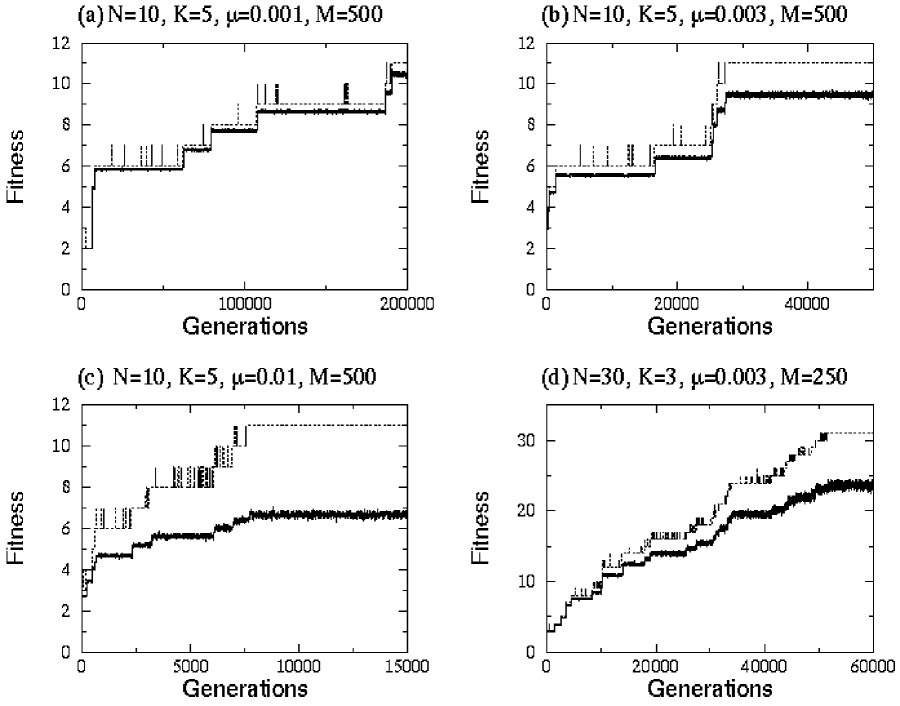
FIG. 5.: Four runs of the Royal Road with Ditches population dynamics with four different parameter settings. The upper dashed lines plot best fitness and the lower solid lines, average fitness ${\langle f\rangle}$ in the population as a function of time, measured in generations. The parameter settings for each run are indicated above each figure. All fitness functions have barriers with a width of $w=2$ and a height of $h=1$. The values of the average fitnesses were obtained by taking a running average over $10$ generations. This reduces the relatively large fluctuations in average fitness between successive generations.

The qualitative dynamics follows the typical alternation of long periods of stasis (epochs) in the average population fitness and short bursts of innovation to higher average fitness; a class of evolutionary dynamics that we call epochal evolution [29]. At the beginning of a run the average and best fitness are low. This simply reflects the fact that high-fitness genotypes are very rare in genotype space and therefore do not occur in an initial random population. A balance is quickly established between selection and mutation that leads to a roughly constant average fitness in the population. This period of stasis we call an epoch. After some time, a mutant may cross the fitness barrier and discover a portal, i.e., a higher-fitness genotype. Relatively frequently, this high-fitness mutant is lost through sampling fluctuations or deleterious mutations. Such events are seen as isolated spikes in the best fitness in Fig. 5. Eventually, one of these beneficial mutants spreads through the population—an innovation occurs. At this point the average fitness increases, until a new equilibrium between selection and mutation is established.

Although many properties of epochal evolution can be treated analytically [30], here we will focus solely on the epoch times. These are the average times between the start of a given epoch and the start of the next. Average epoch times can be obtained from simulation data by tracing backward in time the behavior of the population’s best fitness. The population dynamics runs until genotypes of the highest possible fitness $N+1$ have established themselves in the population for an extended period of time. (For certain parameter settings—specifically, those beyond the error threshold—genotypes with the highest fitness may not stabilize in the population at all. For such parameter settings, an epoch time can be effectively infinite. We will not consider such parameter settings explicitly here.) From there we trace backwards the last time $t_{n}$ that fitness $n$ was the highest in the population, for all values of $n$. The differences $t_{n}-t_{n-1}$ give the epoch times $\tau_{n}$. Some fitness levels may not occur during a run. For instance, in Fig. 5(a) fitness $f=1$ never occurs, since the population starts out with genotypes of fitness $2$. The epoch time $\tau_{1}$ is therefore $0$ for this particular run. Average epoch times are then estimated by averaging the epoch time $\tau_{n}$ over an ensemble of runs. In the following we calculate analytical approximations to these epoch times $\tau_{n}$, using the results from the preceding development.

D Epoch Quasispecies and The Statistical Dynamics Approach

In order to approximate epoch times analytically, we need to determine the average proportion of the population at highest fitness during each epoch. This is the equivalent of $P_{\Pi}$ in Sec. III. From this we can estimate the rate of creation of genealogies in the ditch between the neutral networks of two successive epochs. Then we need to calculate the average population fitness during each epoch to determine the average life time of these ditch genealogies. For the fitness functions studied in the Sec. III these quantities were relatively straightforward to calculate. There, individuals were either on the peak or in the valley, at a certain distance from the portal. For the Royal Staircase with Ditches fitness functions the situation is more complicated.

In principle, one can calculate the current equivalent of $P_{\Pi}$ by representing the population as a distribution of genotypes and calculating metastable genotype distributions for each epoch. This is typically done in population genetics models [9] and in the standard quasispecies models of molecular evolution [7]. However, since genotype spaces are typically very large, an analytical treatment that explicitly takes into account finite-population effects is generally infeasible within this genotypic representation. To address this problem, we introduced an alternative approach that we call statistical dynamics [4, 29, 30]. There one chooses a relatively small number of macroscopic variables with which to describe the population at any given time. Other degrees of freedom are then averaged out using a maximum entropy method similar to the Gibbs method from statistical mechanics. We will use this approach below and simply refer the reader to Refs. [4] and [30] for more extensive treatment of statistical dynamics and a discussion of the relation of this approach to standard quasispecies theory, mathematical population genetics, and other theories from the field of evolutionary computation [25].

We represent the population state at any point in time by a fitness distribution. That is, instead of describing the population by the relative frequencies of all genotypes in the population, we describe it by the relative frequencies of different fitness values. Of course, a given fitness distribution does not uniquely specify a population of genotypes. In order to construct the dynamics on the level of fitness distributions, we must “average out” the additional genotypic degrees of freedom somehow. We do this by assuming, at each generation, a maximum entropy distribution of genotypes given the distribution of fitness. In the Royal Staircase with Ditches fitness functions, this translates into assuming that each string with a given fitness $f$ is equally likely to be any of the genotypes with fitness $f$. That is, a genotype with fitness $n$ will have its first $n-1$ blocks each in a specific state. Blocks $n$ through $N$ are assumed to occur in any of their $2^{K}$ possible states with equal probability. Similarly, for a “ditch” genotype with fitness $n-h$, there are $n-1$ blocks in fixed genotypic states and one block of type $*$. We assume this $*$-block occurs in any of its $2^{K}-2$ possible bit configurations with equal probability. Similarly, we assume that blocks $n+1$ through $N$ are equally likely to be in any of their $2^{K}$ configurations. That is, we assign equal probability to all genotype distributions that are consistent with the given fitness distribution. Since we know the dynamics on the genotype level, we can construct the expected dynamics on the level of fitness distributions under these assumptions.

Formally, we represent the population at time $t$ as a vector $\vec{P}(t)$ with components $P_{n}(t),n=1,2,\ldots,N+1$ that denote the proportion of fitness-$n$ individuals in the population and with components $P_{n,*}(t)$ that denote the proportion of fitness $n-h$ individuals in the ditch between fitness $n$ and fitness $n+1$ genotypes. (Note that in the cases where $h$ is an integer the distribution $\vec{P}(t)$ is not simply a fitness distribution, since it distinguishes ditch individuals from nonditch individuals at the same fitness.)

We then construct a generation operator ${\bf G}$, similar to the one in section III A, that acts on a fitness distribution $\vec{P}(t)$ and returns the expected fitness distribution $\langle\vec{P}(t+1)\rangle$ at the next generation. That is, the dynamics at the level of fitness is to be given by

$$\langle\vec{P}(t+1)\rangle=\frac{{\bf G}\cdot\vec{P}(t)}{{\langle f\rangle}}~{},$$ (71)

where ${\langle f\rangle}$ is the average fitness in the population.

During epoch $n$, in which the best fitness occurring in the population is $n$, there will be a roughly constant fitness distribution $\vec{P}^{n}$. These vectors $\vec{P}^{n}$ are the solutions of the fixed point equations $\langle\vec{P}(t+1)\rangle=\vec{P}(t)$ determined by Eq. (71). Once the operator ${\bf G}$ is constructed, the epoch distribution can be calculated quite easily. More specifically, in Refs. [29] and [30] we showed that the metastable fitness distribution that occurs during epoch $n$ is determined by projecting the operator ${\bf G}$ onto all dimensions with fitness smaller than or equal to $n$ and calculating the principal eigenvector of this projected operator. Determining the epoch-$n$ quasispecies reduces, in this way, to finding the principal eigenvectors of the matrix ${\bf G}$ restricted to components with fitness lower than or equal to $n$. In App. A the generation operator ${\bf G}$ for the Royal Staircase with Ditches is constructed explicitly, and analytical approximations to the epoch quasispecies distributions $\vec{P}^{n}$ are calculated as well. Since the expressions we find for the fitness distributions $\vec{P}^{n}$ are rather cumbersome and we will not give them here.

E Crossing the Fitness Barrier

With the analytical expressions for the epoch fitness distributions $\vec{P}^{n}$ in hand, we can calculate the expected epoch times $\tau_{n}$. An epoch ends via an innovation—a process that proceeds in two stages. First, a portal genotype of fitness $n+1$ is created. And second, this beneficial mutant spreads through the population, rather than being lost.

In order to calculate the average time until a portal genotype is discovered we calculate the probability $P^{\rm seed}$ that a single selection plus mutation from the current population seeds a new lineage that discovers the portal. That is, either by creating a new lineage in the ditch that discovers the portal or else by producing a jump mutation that becomes a portal genotype at once.

This calculation is very similar to that in Sec. III. First of all, the portal is unlikely to be discovered by anything other than either a jump mutation from a fitness-$n$ individual or by a mutation from a ditch genotype. Moreover, ditch lineages are very unlikely to be seeded by anything other than mutants of fitness-$n$ genotypes. Therefore, we can write $P^{\rm seed}$ as

$$P^{\rm seed} = \frac{nP^{n}_{n}(1-\mu)^{(n-2)K}}{f_{n}2^{K}}$$ (72)

$$\times \sum_{i=0}^{K}\epsilon_{i}\left({\rm M}_{iw}-(1-\mu)^{K}\delta_{iw}\right)~{}.$$ (73)

The first factor $nP^{n}_{n}/f_{n}$ gives the probability that a fitness $n$ individual is selected. For the offspring of this individual to end up in the ditch, its $n$th block should be type $A$ (thereby contributing the factor $2^{-K}$) and its first $n-2$ blocks should be left undisturbed by mutation (corresponding to the factor $(1-\mu)^{(n-2)K}$). The terms within the sum give the probability that a valley lineage is seeded by mutation of the $(n-1)$st block at Hamming distance $i$ from the portal. Finally, the factors $\epsilon_{i}$ give the probabilities that a lineage, starting at Hamming distance $i$ from the portal, discovers the portal. They are analogous to the $\epsilon_{i}$ of Sec. III B. Note that the term $\epsilon_{0}{\rm M}_{0w}=1\cdot\mu^{w}(1-\mu)^{K-w}$ corresponds to a jump mutation from a fitness-$n$ genotype directly to a portal configuration. Again, changes to blocks $n+1$ through $N$ are immaterial.

The $\epsilon_{i}$ are calculated paralleling the development in Sec. III B. The only differences are that the genotype length $L$ is now the block length $K$ here, since we are only interested in mutations in the $(n-1)$st block, and that the average number of offspring is slightly modified. The average number of ditch offspring $r$ that an individual in the ditch produces on average is given by

$$r=\frac{(n-d)(1-\mu)^{(n-1)K}}{f_{n}}=\frac{n-d}{n}~{}.$$ (74)

The expressions for the $\epsilon_{i}$ in this case can be obtained by replacing the factor $1/{\langle f\rangle}$ in the equations in Sec. III B by $r$.

Eq. (73) can be further simplified and we eventually obtain the result that

$$P^{\rm seed} =$$ (75)

$$- \frac{P^{n}_{n}}{2^{K}}\left[\epsilon_{w}+\frac{n}{(1-\mu)^{K}(n-d)}\log(1-\epsilon_{w})\right]~{},$$ (76)

where $\epsilon_{w}$ is given by Eqs. (18) and (19) and $P^{n}_{n}$ is determined as outlined in App. A.

Thus, once we have calculated $\epsilon_{w}$ using the results of Sec. III B and calculated $P^{n}_{n}$ using the derivation described in App. A, we find that the average number $g_{n}$ of epoch-$n$ generations until a genotype of fitness $n+1$ is created is given by

$$g_{n}=\frac{1}{1-(1-P^{\rm seed})^{M}}.$$ (77)

In this, we have neglected the correction term $\langle dt\rangle$ of Sec. III D for the time between the seeding of the ditch lineage that leads to the discovery of the portal and the actual time at which the portal is discovered.

We now must calculate the second stage of epoch termination; namely, the probability $\pi_{n}$ that a newly discovered mutant of fitness $n+1$ spreads through the population. In Ref. [30] we showed how a diffusion equation approach [17, 18] can be used to estimate this probability. Applying this here, the probability $\pi_{n}$ that a mutant of fitness $n+1$ will spread through the population is given by:

$$\pi_{n}=1-\exp\left(-2\frac{(n+1)(1-\mu)^{K}}{n}+2\right)~{}.$$ (78)

A mutant must be discovered $1/\pi_{n}$ times on average before it stabilizes and spreads through the population. Thus, $g_{n}/\pi_{n}$ gives the average number of generations until a portal genotype is discovered that spreads through the population—an innovation.

Finally, we have to account for the possibility that epoch $n$ does not occur at all during a run. Only a fraction $P_{e}(n)$ of the runs contain epoch $n$, since, if a higher-fitness genotype occurs in the initial random population, epoch $n$ will be skipped. The proportion $P_{e}(n)$ is simply the probability that no genotypes of fitness greater than $n$ occur in the initial population. This is given by

$$P_{e}(n)=\left[\sum_{i=0}^{n-1}\frac{1}{2^{Ki}}\left(1-\frac{1}{2^{K}}\right)\right]^{M}~{}.$$ (79)

Putting Eqs. (77), (78), and (79) together, the theoretical predictions for the epoch times $\tau_{n}$ become

$$\tau_{n}=P_{e}(n)\frac{g_{n}}{\pi_{n}}~{}.$$ (80)

F Theoretical and Experimental Epoch Times

We tested the predictions of Eq. (80) against experimentally obtained average epoch times for the same parameter settings used in Fig. 5. The results are shown in Fig. 6. Epoch times $\tau_{n}$ are shown as a function of epoch number $n$. The dashed lines give the theoretical predictions of Eq. (80) and the solid lines, the experimentally estimated averages. The data in Fig. 6(a) is an average over $150$ evolutionary runs. All other plots are averages over $250$ runs. The fluctuations in the experimental lines indicate that there is a large variance of epoch times between runs and that, therefore, the raw data is rather noisy. Despite this, the figure demonstrates that the theory estimates epoch times quite accurately.

First, these results show that the analysis presented in Sec. III can be usefully applied to more complicated fitness functions that posses many fitness and entropy barriers. For simplicity in the present case, we restricted ourselves to fitness functions with barriers of equal height and width. However, since our statistical dynamics methods analyze epochs in a piecewise manner, the theoretical results easily extend to more general cases with barriers of variable width and height. The essential ingredient of the analysis is still the genealogy statistics of valley lineages in the ditch that connects to portal genotypes. The only additional ingredients required by the analysis for more complicated cases are (i) the rate of creation of new lineages in the ditch and (ii) the distribution of Hamming distances to the portal at which these lineages are seeded. In the case of the Royal Staircase with Ditches, this was largely determined by the proportion $P^{n}_{n}$ of fitness $n$ individuals during each epoch $n$. Apart from this determining factor, the actual crossing of fitness barriers is still governed by the scaling relations presented in Sec. III F. In particular, the qualitative remarks at the end of Sec. III F still hold in these more general settings. Epoch times grow very rapidly with barrier width and quite slowly with barrier height.

FIG. 6.: Experimentally estimated (solid lines) and theoretically predicted (dashed lines) epoch times $\tau_{n}$ for the four different parameter settings of Fig. 5 as a function of epoch number $n$. All fitness functions have ditches of width $w=2$ and height $h=1$. The experimental epoch times are an average over $150$ runs for Fig. (a) and over $250$ runs for Figs. (b), (c), and (d).

Second, and perhaps of more immediate interest, the general shape of the curves in Fig. 6 reveals several novel population dynamical phenomena. For the lower mutation-rate runs (Figs. 6(a), 6(b), and 6(d)), the epoch times show a distinct break between the relatively small $\tau_{1}$ and the much larger $\tau_{2}$. This jump simply reflects the fact that for these population sizes, it is very likely that individuals with fitness $2$ occur in the initial random population. Due to this, epoch $1$ is skipped most of the time. However, individuals of fitness $3$ are unlikely to occur in the initial population—the occurrence of a fitness $3$ individual is roughly one in $10^{3}$—so that the second epoch is not skipped. In Fig. 6(a) and 6(b), the epoch time curve reaches a maximum after this quick jump and then drops off slightly. In Fig. 6(a) with mutation rate $\mu=0.001$ the times seem to just reach a minimum around the last epoch, number $10$. The curves in Fig. 6(b) reach a minimum epoch time somewhere around epoch $5$ and then start increasing again. The behavior typically occurs for a range of parameter values with low mutation rates and with block sizes $K$ that are not too small. For instance, the theoretical analysis predicts that if there were more than $10$ blocks in the case of Fig. 6(a), then the curve would start to rise after epoch $10$.

Qualitatively, this behavior can be understood as follows. Since the barriers all have equal height $h$, the barriers at later epochs are relatively more shallow than those visited during early epochs. From the analysis in the last section recall that the average number of offspring that ditch individuals produce in the ditch is $r=(n-h)/n$. As $n$ increases, this number approaches $1$ from below. That is, ditch lineages survive longer for later epochs. This effect, of course, decreases epoch times, and this causes the initial decrease of epoch times in Figs. 6(a) and 6(b). However, the ditch lineages are seeded by mutants of fitness-$n$ individuals. For later epochs, fitness $n$ individuals have many more bits, $(n-1)K$, that need to be set to specific configurations. They are, therefore, more likely to undergo deleterious mutations. The proportion $P^{n}_{n}$ of fitness-$n$ individuals during epoch $n$ thus decreases as a function of $n$. This tends to increase the epoch times since smaller $P^{n}_{n}$ implies a lower rate of seeding of ditch lineages. Moreover, the probability $\pi_{n}$ that a genotype of fitness $n+1$, once found, spreads through the population decreases as $n$ increases as well. Eventually, these effects start to dominate, and epoch times start rising again. In fact, at a certain point, for large $n$, the probability $\pi_{n}$ may become so small that fitness-$n+1$ individuals cannot be stabilized in the population at all. In this regime, the dynamics again reaches the well known error threshold: the population dynamics cannot store the necessary $nK$ bits of information that define epoch $n+1$.

In Figs. 6(c) and 6(d), there is no initial decrease of epoch times: the epoch times increase monotonically as a function of $n$. In this case, from the start of the runs the decrease of $\pi_{n}$ and $P^{n}_{n}$ with $n$ dominates the effect of the relatively shallower ditches.

FIG. 7.: Comparison of the entropy- and fitness-barrier crossing times for the Royal Staircase with Ditches fitness function. The dashed line gives the epoch times for the case of minimal width ($w=2$) ditches of height $h=1$. This data is the same as that in Fig. 6(b). The solid lines plot the entropy-barrier epoch times for a fitness function without ditches ($w=0$) for several different block lengths: $K=5$, $9$, $11$, and $12$. All other parameters are identical to the ditch-case parameters: i.e., $N=10$ blocks, a mutation rate of $\mu=0.003$, and a population size of $M=500$. The vertical axis is shown on logarithmic scale.

Finally, we compare these epoch times, for ditches of height $h=1$ and width $w=2$, with the epoch times for the entropy-barrier case ($w=0$) at different block lengths $K$. This comparison is shown in Fig. 7. Epoch times $\tau$ are shown on a logarithmic scale. The dashed line shows the experimentally obtained data for the ditch case with $N=10$ blocks of length $K=5$, a (minimal) ditch width of $w=2$, and height of $h=1$, a population size of $M=500$, and a mutation rate of $\mu=0.003$; as used in Fig. 6(b). The solid lines show experimentally estimated epoch times for the neutral case ($w=0$), for several different block lengths. All other parameters are the same.

In comparing the solid line for $K=5$ with the dashed line we see that the introduction of this minimal ditch increases the epoch times by factors ranging from $50$ to $250$. In order to obtain roughly comparable epoch times for the neutral case $w=0$, one has to increase the block length to as high as $K=12$. This demonstrates how much more rapidly entropy barriers are crossed than fitness barriers. In the time that it takes the population to cross a fitness barrier of width $w=2$, the neutrally diffusing population will have crossed an entropy barrier of an additional $12-5=7$ bits. Thus, the neutrally diffusing population explores roughly $2^{7}=128$ times as many different neutral configurations in the time that it takes to cross the $2$-bit fitness barrier. As we will see below, the difference in time scale for crossing fitness and entropy barriers grows much larger for more realistic (lower) mutation rates and (longer) sequences.

VI Conclusions

We analyzed in detail the barrier crossing dynamics of a population evolving under selection and mutation in a constant selective environment. Barriers of two distinct types exist: fitness barriers and entropy barriers. Fitness barriers occur in a fitness “landscape” when genotypes of higher fitness than currently present in the population are separated from the current most-fit genotypes by valleys of lower fitness. In order for such barriers to be crossed, a rare sequence of mutants must cross the valley of low-fitness genotypes. The second type of barrier, entropy barriers, occurs when genotypes of current best-fitness form large neutral networks in genotype space that only have a small number of connections (portals) to genotypes of higher fitness. Evolving populations diffuse at random through these neutral subbasins under selection and mutation. Since connections to higher fitness genotypes are rare, the population must search and spread over large parts of the neutral network, before higher-fitness genotype portals are discovered.

We will now qualitatively and quantitatively summarize the general picture that has emerged from our analysis of barrier crossing dynamics. The first important observation to be made is that there is a large qualitative difference between the genealogies of individuals of current best fitness and those with suboptimal fitness. All suboptimal individuals in the population are relatively recent descendants of genotypes with the current highest fitness. In other words, individuals with suboptimal fitness only give rise to genealogical bushes—genealogies of finite, typically short, length. Individuals with the current highest fitness are the only ones that give rise to lineages of potentially infinite length.

More formally, let us denote by $\Lambda$ the neutral network of genotypes whose fitness equals that of the current highest-fitness individuals. The subpopulation of the current population that is on the neutral network $\Lambda$ then effectively acts as a source for the whole population’s descendants. Genealogies of lower-fitness individuals outside of $\Lambda$ go extinct relatively quickly and are replaced by new genealogies that are mutant descendants of individuals on the neutral network $\Lambda$. Therefore, only lineages of individuals on the network $\Lambda$ can “travel” long distances through genotype space. The subpopulation of genotypes in $\Lambda$ diffuses randomly through $\Lambda$, eventually visiting almost all genotypes in $\Lambda$ and all of their single mutant neighbors.

At the same time, the excess reproduction of individuals in $\Lambda$, combined with deleterious mutations, creates individuals in the lower-fitness valleys or ditches around $\Lambda$. These individuals then give rise to genealogies of valley individuals that, in turn, probe at random the genotype space surrounding $\Lambda$. However, since these valley genealogies typically go extinct quite rapidly, individuals in the valley never travel far from the neutral network $\Lambda$. That is, only those parts of the valleys that are in the immediate neighborhood of the neutral network $\Lambda$ will be quickly explored. Valley genealogies that cross a wide valley are very rare.

Therefore, on the shortest time scale, the population explores the neutral network $\Lambda$ and its neighborhood, as shown in Fig. 2. If there are any higher-fitness genotypes in the immediate neighborhood of the network $\Lambda$, the population is most likely to escape from the metastable state (epoch) by crossing this entropy barrier. If the neutral network $\Lambda$ is completely surrounded by valleys of lower fitness, the population will eventually escape from the metastable state when a mutant crosses one of the valleys that surrounds $\Lambda$, i.e., by crossing a fitness barrier. Since the waiting time for such a fitness barrier crossing increases very rapidly with the width of the barrier, it is most likely that the escape will occur along one of the narrowest valleys that connects $\Lambda$ to higher fitness genotypes. Although shallow valleys are more easily crossed than deep valleys, the effect of barrier height is relatively small compared to the effect of barrier width.

This basic picture of the metastable population dynamics is captured more quantitatively by the scaling relations of Eqs. (44) and (64) for the fitness-barrier and entropy-barrier crossing times, respectively. By equating these, we get a rough comparison of the trade offs in the crossing of entropy versus fitness barriers. To make the comparison for more general cases, we replace the factor $2^{L}$ in the entropy-barrier scaling form, Eq. (64), with $V_{\Lambda}$ to denote the volume of the neutral network $\Lambda$. We also replace $L$ by the average neutrality $\nu$—i.e., the average number of neutral neighbors—of genotypes in $\Lambda$. This extends the entropy-barrier scaling form to more general neutral network topologies than simple binary hypercubes. We then obtain

$$V_{\Lambda}=\frac{\nu}{w!}\left(\frac{\log(\sigma)}{\mu}\right)^{w-1}~{}.$$ (81)

This is an estimate of the volume $V_{\Lambda}$ of the network $\Lambda$ that is explored in the time it takes the population to cross a fitness barrier of height $\sigma$ and width $w$.

Recall that the factor $w!$ denotes the number of different paths leading across the fitness barrier and that $\mu/\log(\sigma)$ gives the average number of mutations valley lineages undergo before they go extinct. The relative size of $\mu$ and $\log(\sigma)$, together with the barrier width $w$, are the decisive quantities. Only when $\mu/\log(\sigma)$ approaches $1$ can fitness barriers be crossed relatively quickly. However, since $\mu$ is typically very small, even in cases where the highest-fitness genotypes have only a small fitness advantage over valley genotypes—i.e., $\sigma=1+\epsilon$—the determining ratio $\mu/\epsilon$ may still be small.

As an illustration, assume that each genotype in $\Lambda$ has an average of $\nu=60$ neutral neighbors, that the mutation rate is $\mu=10^{-6}$, and that genotypes in $\Lambda$ are on average $1$ percent more fit than genotypes in the valley. Substituting these values into Eq. (81) for a barrier of width $w=3$, we find $V_{\Lambda}\approx 10^{9}$. Thus, before this fitness barrier will be crossed, on the order of $10^{9}$ genotypes on the neutral network $\Lambda$ will have been explored. Of course, these numbers should not be taken as quantitative predictions, they are only rough order-of-magnitude estimates. However, they do indicate the difference in time scales at which entropy and fitness barriers are crossed.

In cases where the fitness advantage $\epsilon$ becomes so small as to be comparable in size to $\mu$, the fitness barrier will have effectively turned into an entropy barrier. That is, for such small fitness advantages, selection is not able to stabilize the population within $\Lambda$ and the population will freely diffuse through the valleys. In short, before $\epsilon$ becomes so small as to be comparable to $\mu$, the population will have already crossed the error threshold. This can be seen, for instance, by taking the logarithm on both sides in Eq. (46).

As we discussed earlier, the picture of the barrier crossing dynamics that has emerged from our analysis contrasts strongly with the common view that this process is analogous to the dynamics of energy-barrier crossing in physical systems. In those systems, the stochastic dynamics follows the local gradient of the energy landscape. This local character of the dynamics causes the barrier height to be the main determinant of the barrier crossing time. Generally, the evolutionary population dynamics cannot be described as following a local gradient. The current highest fitness of the individuals located on the neutral network $\Lambda$ sets an absolute fitness scale against which valley individuals must compete. Therefore, valley lineages are unlikely to survive for many generations and so cannot undergo many mutations before going extinct. This mechanism causes the barrier width to be the main determinant of the fitness-barrier crossing time in population dynamics.

The preceding results demonstrate the important role of neutral networks in genotype space for evolutionary dynamics: where a population goes in genotype space is largely determined by the available neutral paths.

A Analytical Approximation of the Epoch Quasispecies

In this appendix, we construct the generation operator ${\bf G}$ for the class of Royal Staircase with Ditches fitness functions, and analytically approximate the metastable quasispecies distributions $\vec{P}^{n}$.

As before, the operator ${\bf G}$ decomposes into a part ${\bf S}$ that encodes the expected effects of selection on the population fitness distribution and a mutation operator ${\bf M}$ that encodes the expected effects of mutation.

The selection operator $\bf S$ is easy to construct since selection depends only on the population’s fitness distribution. After selection, we have for the nonditch genotypes that:

$$P^{\rm sel}_{n}\equiv\frac{\left({\bf S}\cdot\vec{P}\right)_{n}}{{\langle f\rangle}}=\frac{n}{{\langle f\rangle}}P_{n}~{},$$ (A1)

and for the ditch genotypes that

$$P^{\rm sel}_{n,*}=\frac{n-h}{{\langle f\rangle}}P_{n,*}~{}.$$ (A2)

Construction of the mutation operator ${\bf M}$ is more involved, but straightforwardly follows Ref. [30]. Formally, the probability ${\rm M}_{ij}$ that a genotype of type $j$ turns into a genotype of type $i$ under mutation is given by a sum over all genotypes of type $i$ and $j$, weighted by the probability of mutating from one genotype to the other. When we refer to the “type” of a genotype we distinguish genotypes only based on their location in an epoch’s neutral network ($n$) or intervening ditch ($n,*$). We denote by $\Lambda_{i}$ the set of all genotypes of type $i$ and by $d(s,s^{\prime})$ the Hamming distance between the genotypes $s$ and $s^{\prime}$. Formally, we then have:

$${\rm M}_{ij}=\sum_{s\in\Lambda_{i}}\sum_{s^{\prime}\in\Lambda_{j}}\frac{\mu^{d(s,s^{\prime})}(1-\mu)^{L-d(s,s^{\prime})}}{|\Lambda_{j}|}~{},$$ (A3)

where $|\Lambda_{j}|$ is the size of the set $\Lambda_{j}$. That is, we assume that a type $j$ genotype is equally likely to be any of its possible $|\Lambda_{j}|$ genotypes. We then sum over all possible genotypes of type $i$ to which $j$ can mutate. The generation operator ${\bf G}$ is then, as before, the product of the selection operator, Eqs. (A1) and (A2), and the resulting mutation operator: ${\bf G}={\bf M}\cdot{\bf S}$.

We now list expressions for the different types of ${\bf G}$’s components. In order to simplify the formulas, we first define

$$\alpha=\left(\frac{\mu}{1-\mu}\right)^{w}~{},$$ (A4)

and the probability $\lambda$ to not mutate a block, which is given by

$$\lambda=(1-\mu)^{K}~{}.$$ (A5)

Using this notation, the probability to mutate a block from type $A$ to type $B$, for instance, becomes ${\rm Pr}(A\rightarrow B)=\alpha\lambda$. Components $G_{ij}$ with $i<j$ become

$$G_{ij}=\alpha\lambda^{i-1}j~{},$$ (A6)

for $i\neq 1$, and

$$G_{1j}=\left(1-\lambda^{j-1}-\alpha\frac{\lambda-\lambda^{j-1}}{1-\lambda}\right)j~{},$$ (A7)

for $i=1$. The diagonal components are given by

$$G_{jj}=\lambda^{j-1}j~{}.$$ (A8)

For the ditch genotypes, the diagonal components are:

$$G_{(j-h)(j-h)}=\lambda^{j-1}(j-h)~{}.$$ (A9)

Components describing the transitions from ditch genotypes to lower-fitness nonditch genotypes $i<j$ are given by:

$$G_{i(j-h)}=\alpha\lambda^{i-1}(j-h)~{}.$$ (A10)

Finally, mutations from nonditch genotypes to lower lying ditch genotype come in three varieties. First, for $i<j-2$ we have

$$G_{(i-h)j}=\alpha\lambda^{i-1}(1-\lambda-\lambda\alpha)j~{}.$$ (A11)

For $i=j-1$ we have

$$G_{(j-1-h)j}=\lambda^{j-2}(1-\lambda-\alpha\lambda)j~{}.$$ (A12)

And for the ditch lying immediately below, $i=j$, we have

$$G_{(j-h)j}=\frac{1}{2^{K}}\lambda^{j-2}(1-\lambda-\alpha\lambda)j~{}.$$ (A13)

The quasispecies fitness distribution during epoch $n$ is given by the principal eigenvector of the matrix ${\bf G}$ restricted to the components with fitness lower than or equal to $n$; see Refs. [29] and [30]. This eigenvector can be obtained numerically, using the above formulas for the components $G_{ij}$.

An analytic approximation to $\vec{P}^{n}$ can be obtained by considering mutations only from each fitness $j$ (or $j-h$) to equal or lower fitness. This approximation is justified by the fact that fitness-increasing mutations are very rare compared to fitness-decreasing mutations. Under that approximation, the matrix ${\bf G}$ becomes upper triangular. For upper triangular matrices, the components $\vec{P}^{n}_{i}$ of the principal eigenvector $\vec{P}^{n}$ obey the equations:

$$P^{n}_{i}=\frac{\sum_{j>i}^{n}G_{ij}P^{n}_{j}}{G_{nn}-G_{ii}}~{},$$ (A14)

and, since $\vec{P}^{n}$ is a distribution, we additionally have the normalization condition given by

$$\sum_{i=1}^{n}P^{n}_{i}=1~{}.$$ (A15)

Note that the sums in the above equations involve both ditch genotypes and nonditch genotypes. Their precise ordering with respect to fitness depends, of course, on the barrier height $h$. For instance, for $0<h<1$, the fitness $n-h$ genotypes in the ditch between fitness-$n$ and fitness-$(n+1)$ genotypes lie between fitness $n-1$ and $n$.

With the analytic expressions for the components of ${\bf G}$ in hand, and by using Eq. (A14), we can express all $P^{n}_{i}$ for $i<n$ as a function of $P^{n}_{n}$. For instance, assuming $h<1$, such that the genotypes of fitness $n-h$ are the second highest-fitness genotypes in the population, we have

$$P^{n}_{n,*}=\frac{n(1-\lambda-\alpha\lambda)}{2^{K}h\lambda}P^{n}_{n}~{}.$$ (A16)

Using this, we have for genotypes of fitness $n-1$ that

$$P^{n}_{n-1}=\frac{n\left(\alpha(n-h)(1-\lambda-\alpha\lambda)+2^{K}\lambda\right)}{\left(1-n(1-\lambda)\right)\lambda 2^{K}}P^{n}_{n}~{}.$$ (A17)

When all components $P^{n}_{i}$ with $i<n$ have been expressed in terms of $P^{n}_{n}$ in this way, one finally uses the normalization condition Eq. (A15) to determine $P^{n}_{n}$.

This procedure leads in a straightforward way to a relatively accurate analytical expression for the epoch fitness distributions. The expressions, however, are rather cumbersome and we will not list them all here. In general, they depend on the size of $h$ since the ordering of the fitness values of the different types of genotypes depends on $h$.

REFERENCES

- [1] C. Adami. Self-organized criticality in living systems. Phys. Lett. A, 203:29–32, 1995.
- [2] L. Barnett. Ruggedness and neutrality—the NKp family of fitness landscapes. In C. Adami, editor, ALIFE VI, 1998. Available at: http://www.cogs.susx.ac.uk/users/lionelb/.
- [3] J. P. Crutchfield and M. Mitchell. The evolution of emergent computation. Proc. Natl. Acad. Sci. U.S.A., 92:10742–10746, 1995.
- [4] J. P. Crutchfield and E. van Nimwegen. The evolutionary unfolding of complexity. In L. F. Landweber, E. Winfree, R. Lipton, and S. Freeland, editors, Evolution as Computation, Lecture Notes in Computer Science, page to appear, New York, 1999. Springer-Verlag. Santa Fe Institute Working Paper 99-02-015; adap-org/9903001.
- [5] B. Derrida and L. Peliti. Evolution in a flat fitness landscape. Bull. Math. Bio., 53(3):355–382, 1991.
- [6] M. Eigen. Self-organization of matter and the evolution of biological macromolecules. Naturwissen., 58:465–523, 1971.
- [7] M. Eigen, J. McCaskill, and P. Schuster. The molecular quasispecies. Adv. Chem. Phys., 75:149–263, 1989.
- [8] S. F. Elena, V. S. Cooper, and R. E. Lenski. Punctuated evolution caused by selection of rare beneficial mutations. Science, 272:1802–1804, 1996.
- [9] Warren J. Ewens. Mathematical population genetics, volume 9 of Biomathematics. Springer-Verlag, 1979.
- [10] W. Fontana and P. Schuster. Continuity in evolution: On the nature of transitions. Science, 280:1451–5, 1998.
- [11] H. Frauenfelder, editor. Landscape Paradigms in Physics and Biology. Concepts, Structures and Dynamics (Papers originating from the 16th Annual International Conference of the Center for Nonlinear Studies. Los Alamos, NM, USA, 13-17 May 1996), Amsterdam, 1997. Elsevier Science. Published as a special issue of Physica D 107 no. 2–4 (1997).
- [12] C. W. Gardiner. Handbook of Stochastic Methods. Springer-Verlag, 1985.
- [13] S. J. Gould and N. Eldredge. Punctuated equilibria: The tempo and mode of evolution reconsidered. Paleobiology, 3:115–251, 1977.
- [14] T. E. Harris. The theory of branching processes. Dover publications, New York, 1989.
- [15] M. Huynen, P. F. Stadler, and W. Fontana. Smoothness within ruggedness: The role of neutrality in adaptation. Proc. Natl. Acad. Sci. USA, 93:397–401, 1996.
- [16] S. A. Kauffman and S. Levin. Towards a general theory of adaptive walks in rugged fitness landscapes. J. Theo. Bio., 128:11–45, 1987.
- [17] M. Kimura. On the probability of fixation of mutant genes in a population. Genetics, 47:713–719, 1962.
- [18] M. Kimura. Diffusion models in population genetics. J. Appl. Prob., 1:177–232, 1964.
- [19] M. Kimura. The neutral theory of molecular evolution. Cambridge University Press, 1983.
- [20] R. Lande. Expected time for random genetic drift of a population between stable phenotype states. Proc. Natl. Acad. Sci. USA, 82:7641–7645, 1985.
- [21] C. A. Macken and A. S. Perelson. Protein evolution in rugged fitness landscapes. Proc. Nat. Acad. Sci. USA, 86:6191–6195, 1989.
- [22] C. M. Newman, J. E. Cohen, and C. Kipnis. Neo-darwinian evolution implies punctuated equilibrium. Nature, 315:400–401, 1985.
- [23] M. Newman and R. Engelhardt. Effect of neutral selection on the evolution of molecular species. Proc. R. Soc. London B., 256:1333–1338, 1998.
- [24] M. Nowak and P. Schuster. Error thresholds of replication in finite populations, mutation frequencies and the onset of Muller’s ratchet. J. Theo. Biol., 137:375–395, 1989.
- [25] A. Prügel-Bennett and J. L. Shapiro. Analysis of genetic algorithms using statistical mechanics. Phys. Rev. Lett., 72(9):1305–1309, 1994.
- [26] N. G. van Kampen. Stochastic Processes in Physics and Chemistry. North-Holland, 1992.
- [27] E. van Nimwegen and J. P. Crutchfield. Optimizing epochal evolutionary search: Population-size dependent theory. Machine Learning, submitted, 1998. Santa Fe Institute Working Paper 98-10-090. adap-org/9810004.
- [28] E. van Nimwegen and J. P. Crutchfield. Optimizing epochal evolutionary search: Population-size independent theory. Computer Methods in Applied Mechanics and Engineering, special issue on Evolutionary and Genetic Algorithms in Computational Mechanics and Engineering, D. Goldberg and K. Deb, editors, in press, 1998. Santa Fe Institute Working Paper 98-06-046. adap-org/9810003.
- [29] E. van Nimwegen, J. P. Crutchfield, and M. Mitchell. Finite populations induce metastability in evolutionary search. Phys. Lett. A, 229:144–150, 1997.
- [30] E. van Nimwegen, J. P. Crutchfield, and M. Mitchell. Statistical dynamics of the Royal Road genetic algorithm. Theoretical Computer Science, special issue on Evolutionary Computation, A. Eiben, G. Rudolph, editors, in press, 1998. SFI working paper 97-04-35.
- [31] G. Weisbuch. Complex Systems Synamics: An Introduction to Automata Networks, volume 2 of Santa Fe Institute Studies in the Sciences of Complexity, Lecture Notes. Addison-Wesley, Reading, Massachusetts, 1991.
- [32] S. Wright. The roles of mutation, inbreeding, crossbreeding and selection in evolution. In Proc. of the Sixth International Congress of Genetics, volume 1, pages 356–366, 1932.
- [33] S. Wright. Character change, speciation, and the higher taxa. Evolution, 36:427–43, 1982.