Noise-induced memory in extended excitable systems

Abstract

We describe a form of memory exhibited by extended excitable systems driven by stochastic fluctuations. Under such conditions, the system self-organizes into a state characterized by power-law correlations thus retaining long-term memory of previous states. The exponents are robust and model-independent. We discuss novel implications of these results for the functioning of cortical neurons as well as for networks of neurons.

Neurons receive thousands of perturbations affecting the transmembrane voltage at various points of the synaptic membrane. Recent experimental evidence has shown active nonlinearities [2] at the dendrites of cortical neurons, and thus implying that a model representing these neurons must have many nonlinear spatial degrees of freedom.

What are the dynamical consequences of these distributed nonlinearities for the neurons function? The answer is not inmediately certain. The prevailing view has been, since Lapicque in 1907 [1], that all input regions (i.e., dendrites) were linear, and thus neurons were represented as a single compartment. In this view incoming excitations are linearly integrated and whenever the resulting value exceeds a predefined threshold an output (action potential) is generated. Thus, the neuron is considered to has a single non-linear degree of freedom (i.e., the spatial region where the thresholding dynamics takes place).

This Letter describes a robust form of noise-induced memory which appears naturally as a direct consequence of including distributed nonlinearities in the formulation of a neuron’s input region. Besides having relevance at the neural level, its touches other areas of biology where excitable models have been used, as is the case for models of forest-fire propagation, spreading of epidemics and noise-induced waves.[3] From the outset, it needs to be noted that the phenomena to be described do not depend of the type of excitable model one uses.

To show the essence of the main point we adapt the Greenberg-Hastings cellular automata model[4] of excitable media[7]. For the purpose of this report let restrict ourselves to the case of a one-dimensional lattice of coupled identical compartments ($n=1,...,N$), with open boundary conditions. Thus, each spatial location is assigned a discrete state $S^{t}_{n}$ which can be one of three: Quiescent, Excited or Refractory, with the dynamics determined by the transition rules: E $\rightarrow$ R (always), R $\rightarrow$ Q (always), Q $\rightarrow$ E (with probability $\rho$, or if at least one neighbor is in the E state), Q $\rightarrow$ Q (otherwise). To introduce the so-called “refractory period” typical of all excitable systems during which no re-excitation is possible, the transition from the R state to the Q state is delayed for $r$ time steps. Thus, the only two parameters in the system are $\rho$, which determines the probability that an input to a given site $n$ result into an excitation (i.e., a transition Q $\rightarrow$ E); and $r$ determining the time scale of recovery from the excited state. It turns out that the precise value of $r$ is not crucial, but choosing a value of $r$ at least equal or larger than the value of $N$ eliminates a number of numerical complications [6]. A dendritic region bombarded by many weak synaptic inputs is simulated adopting a relatively small value for $\rho$ (here $10^{-2}$). The typical response of the model under such conditions is illustrated in Fig. 1. One can see that, starting from arbitrary initial conditions, eventually an element is first excited (left arrow in Fig. 1). This initiates a propagated wavefront which collides with others initiated in the same way somewhere else in the system. After the completion of the refractory period the process repeats originating another wavefront (right side of Fig. 1). An inmediately apparent feature is the overall similarity of any two consecutive fronts. The large-scale shape is preserved, despite of the fact that each element is being randomly perturbed.

We found that important information can be extracted from the analysis of the dynamics of the first element to be excited in each wavefront, denoted as $L(n)$. Figure 2 shows results of numerical simulations where $L(n)$ of each wavefront is plotted as a function of time. Note the tendency of $L(n)$ to remain near the previous leading site, which is specially apparent in the larger systems. To quantify this dynamics we estimated numerically $<|L^{t}(n)-L^{t+1}(n)|>$ which is how far (on average) from its current position the leader will be in the next wavefront. The resulting distributions $<P(\Delta n)>$ of these jumps are plotted in Figure 3A for all systems sizes. The largest probability corresponds to the case in which the wavefront is first triggered from the same element as in the previous event. The power-law $n^{\pi}$ tells us that there is always a non-zero probability for a very long jump, indeed as large as the entire system. Therefore, the cut-off of the power law is the only difference between the results obtained with small or large N (see Panel A in Figure 3) Another related measure is the estimation of the average distance the leader drifts from its current position as a function of time lag $\Delta t$ (t is always given in wavefront’s units). The results are plotted in panel B of Figure 3. The fact that the log-log plot of $|\Delta n|$ vs $\Delta t$ is linear implies a power law $\sim\Delta t^{H}$. The best-fit line of the results in Figure 3B gives an exponent $H=0.19$. For this case it is known that the power spectrum decays as $1/f^{\beta}$ and that $\beta$ relates with $H$ as $\beta=2H+1=1.4$. A random walk will have similar statistical behavior but with an exponent $H=1/2$. These power-laws, with cutoffs given only by the system size, imply a lack of characteristic scale (both in time and space), a situation which resembles some of the scenarios described in the context of self-organized criticality [8].

What causes this memory is trivially simple: the first site to be activated by the noise will necessarily be the first (exactly after $r$ time steps) to be recovered and consequently to be ready to be re-excited. The two adjacent sites which were excited by the leader will recover only after $r+1$ time steps, and so on for the other adjacent sites. Thus, excitation by the noise will always be biased by the previous sequence of excitation. Therefore, this “memory” can be preserved as long as the cycle of recovery (in this model the $r$ time steps) is not affected by the noise. Regarding the dependence with the noise intensity, for vanishingly small $\rho$ all sites will have enough time to cycle to the Q state and no memory will be kept (see below). - Exponents are robust - The phenomenology described as well as its characteristics power laws are not model-dependent. The fact that similar results were obtained with various numerical models motivated the search for the simplest numerical simulation scheme. It turns out that the dynamics and the statistical behaviour is preserved by the simple kinematic description of the motion of these noise-induced propagated excitable waves. The approach is described using the cartoon in Figure 4 as follows: Time and space are considered continuos variables. It is assumed that excitations can initiate a wavefront at any point in the 1D space with uniform probability. Therefore, after choosing the noise amplitude ($\rho$) the first step of the algorithm is to distribute all the potential excitation spots at random location and at random times. Larger values of $\rho$ imply more events to be distributed. Filled circles in Fig. 4 denoted “a” trough “e” correspond to few of these events. Then the space is scanned to locate the earliest excitation point (i.e., in the figure is the point “a” . Subsequently, two wavefronts are drawn from that point with uniform (arbitrary) speed. A front dies when either reaches the boundary as in the initial case or upon colliding with other front as the one initiated by event labeled “b”. (the dotted lines indicate two of these interrupted fronts). Thus the algorithm is the repetition of scanning follows by the identification of potential collisions. It needs to be noted that nothing is peculiar of these rules, simply they are the algorithmic description of what is known about excitable waves. The results of extensive simulations are plotted in Figure 3 side by side with those already described for the discrete model. The jump distributions are plotted for four noise levels in Panel C. The mean drifts as a function of time lag are plotted in Panel D. It can be seen that there is a remarkable agreement between the numerical values of both scaling exponents.

-How long does it remember?- For the sake of demonstration, the dissipation of memory can be estimated by first imposing an initial activation sequence in the system (i.e., writing) and then calculating the Hamming distance between the initial and subsequent wavefront separated by $\Delta t$. Using the discrete model we impose an arbitrary initial configuration of excitation, in this case the sinusoidal pattern plotted in the inset of panel A of Figure 5. As time passes, the pattern deforms as shown by the snapshots at times 2, 5, 10 and 50 in the figure, which can be estimated by the Hamming distance defined as:

$$<D(t)>=\frac{1}{N}\sum_{n=1}^{N}|S^{t}_{n}-S^{t+\Delta t}_{n}|$$ (1)

where $S$ are the initial and subsequent states, ranked by the excitation order of each element. Means and SEM $D(t)$ were calculated and the results are plotted in the main body of Figure 5A as a function of $\rho$. It can be seen that the Hamming distance follows a power-law up to times of about 50 events. It was already mentioned that for vanishingly small $\rho$ no memory of previous states can be maintained since this condition implies that all the element have enough time to go to the Q state preceding the excitation. Thus, rather paradoxically, more noise implies longer memory. This is illustrated by the results in Figure 5B, where $D(t)$ was calculated for increasing noise $\rho$. Thus, we can call this phenomena a form of noise-induced memory.

- Implications for learning and memory - The dynamics described here might have important consequences for neural “plasticity”. This is the name given, in neuroscience, to the process by which interconnected neurons can strengthen or weaken their synaptic contacts to modulate their communication. The dogma is that memory and learning in animal brains are based on long-term changes of the synaptic connectivity. An important point in contemporary thinking assumes that whatever the plastic process is, it must be able to modify the synaptic strength during the time window imposed by the longest time-scale in the neuron dynamics. This window is given by the relaxation kinetics of the membrane and is at most of the order of hundreds of milliseconds [10]. This length is considered too short for producing most of the necessary synaptic changes. The length of that window can be many orders of magnitude longer, if the results presented in this Letter survive the intricate complexity of the spatial structure in real neurons, as well as perhaps other caveats. This would imply that the correlated spatial activity along the dendrites established by the inputs will only decay after hundreds of firing events. This time scale is much longer than the fraction of a second currently considered as the longest time scale that a neuron could remember from its past history. This correlated sequence of activation can in turn influence the spatial distribution of the molecular machinery supposedly responsible for the long-term synaptic modifications.

The work reported here is restricted, for simplicity, to the one dimensional case and the use of the simplest conceivable excitable model. Nevertheless, the phenomena is robust and similar results can be obtained using more detailed models. If the dynamic described here exist as such in real neurons it would be very relevant to neural functioning.

Supported by the Mathers Foundation. R.U. Computer resources are supported by NSF ARI Grants. Discussions with P. Bak, R. Llinas and Mark Millonas are appreciated. Communicated in part by DRC at the First International Conference on Stochastic Resonance in Biological Systems. Arcidosso, Italy, May 5-9, 1998 where the hospitality of the colleagues of the Istituto di Biofisica of Pisa was cherished.

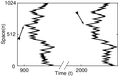
FIG. 1.: An example of two consecutive noise-induced wavefronts. Note the similarity in the overall shape of the two consecutives wavefronts, which is typical. The arrows indicate the earliest activated site (i.e., the leader $L(n)$) in each wavefront.

FIG. 2.: Plot of the consecutive positions of the leading element in each firing event (i.e., the ones identified by the arrows in Fig. 1). The tendency of the leader is to remain near the previous leading site, a fact that is visually more apparent in the large systems. (System size increases from N = 128 at the top to N = 4096 at the bottom panel. $\rho=10^{-2}$ for all panels.)

FIG. 3.: (A and C): Distribution of the differences between $L(n)$ of two consecutive wavefronts. Results in A correspond to the discrete model while results plotted in C are from the kinematic simulation. In both cases the exponent $\pi\sim 1.4$ (B and D): Mean drift of $L(n)$ as a function of time lag $\Delta$t. Results in B are from the discrete model, those plotted in D are from the kinematic simulation. The mean drift scales as $t^{H}$, the best-fit line gives $H=0.19$ in the case of the discrete model and $H=0.2$ for the results using the kinematic description. The system sizes for the discrete model are N = 128, 256, 512, 1024, 2048, 4096 from bottom to top plots, the noise $\rho=10^{-2}$. For the kinematic description system size is fix (unit interval) and noise density increases from bottom to top plots from $10^{-6}$; $10^{-5}$ ; $10^{-4}$;$10^{-3}$.

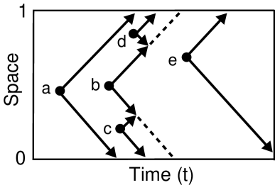
FIG. 4.: Cartoon of the kinematic algorithm (see text).

FIG. 5.: (A): The Hamming distance $<D(t)>$ from the original sinusoidal pattern as a function of time. The inset shows the initial wavefront and at time steps: 2, 5, 10 and 50. $N=256$, $\rho=10^{-2}$ means and SEM of 256 realizations. (B): The Hamming distance between two consecutives wavefront as a function of noise $\rho$. (Means and SEM of 256 realizations).

REFERENCES

- [1] H.C. Tuckwell, Stochastic Processes in the Neurosciences (SIAM, Philadelphia, 1989).
- [2] The reports on the experimental evidence of active channels is gargantuan, but a a recent survey can be found in Z.F.Mainen T.J. Sejnowski ”Modeling active dendritic processes in pyramidal neurons.” In Methods in Neuronal Modeling. Koch, C, and Segev, I. (eds) 2nd ed., pp.171-210. MIT Press: Cambridge, MA (1998).
- [3] S. Kadar, J. Wang, and K. Showalter. Noise Supported Traveling Waves in Subexcitable Media. Nature 391,770-772 (1998).
- [4] J. M. Greenberg and S. P. Hastings. Spatial patterns for discrete models of diffusion in excitable media. SIAM J. Appl. Math. 34(3),515-523,(1978).
- [5] C. Koch, Biophysics of computation, Oxford University Press, New York (1998).
- [6] By considering that in these systems the time to excite the whole system is smaller than the recovery time we could safely assume .
- [7] Other numerical formulations including a explicit integrate and fire scheme give similar results.
- [8] P. Bak, C. Tang, and K. Wiesenfeld, Phys. Rev. Lett. 59, 381 (1987); Phys. Rev. A38, 364 (1988); P. Bak, How nature works: the science of self-organised criticality. (Springer, New York, 1996; Oxford University Press, 1997); M. Paczuski, S. Maslov, and P. Bak, Phys. Rev. E53, 414 (1996).
- [9] B.W. Mel, J. Neurophys. 70,1086-1101 (1993)
- [10] Basically one have to consider the decay to equilibrium of the membrane potential after being perturbed by the synaptic current. A rough figure of hundreds of milliseconds is the current estimate.