[

Extremal Coupled Map Lattices

Abstract

We propose a model for co-evolving ecosystems that takes into account two levels of description of an organism, for instance genotype and phenotype. Performance at the macroscopic level forces mutations at the microscopic level. These, in turn, affect the dynamics of the macroscopic variables. In some regions of parameter space, the system self-organises into a state with localised activity and power law distributions.

PACS: 05.45.+b, 64.60.Lx, 87.10.+e

]

Complex extended systems showing a lack of scale in their features appear to be widespread in nature, being as diverse as earthquakes [3, 4], creep phenomena [5], material fracturing [6, 7, 8], fluid displacement in porous media [9, 10], interface growth [11, 12], river networks [13, 14, 15] and biological evolution [16, 17, 18, 19]. At variance with equilibrium statistical mechanics, these systems do not need any fine tuning of a parameter to be in a critical state. To explain this behaviour, Bak, Tang and Wiesenfeld introduced the concept of self-organised criticality (SOC) through the simple sand-pile model [20, 21]. In recent years, several models with extremal dynamics have been shown to exhibit SOC in the presence of a sufficiently decorrelated signal  [22].

Several years ago, Bak and Sneppen (BS) proposed a SOC model [23] for the co-evolution of species. In the BS model each species occupies a site on a lattice. Each site $j$ is assigned a fitness, namely a random number between $0$ and $1$. At each time step in the simulation the smallest fitness is found. Then the fitnesses of the minimum and of its nearest neighbours are updated according to the rule

$$f_{n+1}=F(f_{n})$$ (1)

that assigns a new fitness $f_{n+1}$ at time $n+1$ to the chosen lattice site. This corresponds to the extinction of the less fit and its impact on the ecosystem. Indeed, in the original BS model, the function $F$ is just a random function with a uniform distribution between 0 and 1. The system reaches a stationary critical state in which the distribution of fitnesses is zero below a certain threshold and uniform above it (the actual value of the threshold depends on the updating rule). It has been shown [24, 25] that the exact nature of the updating rule is not relevant. Indeed, the use of a chaotic map instead of a random update, preserves the universality class (even if the final distribution may be altered).

As a result of the dynamical rules, the BS system exhibits sequences of causally connected evolutionary events called avalanches [23]. The number of avalanches $N$ follows a power law distribution $N(s)\sim s^{-\tau}$ where $s$ is the size of the avalanche and $\tau\sim 1.07$ [22, 26, 27]. Other quantities also exhibit a power law behaviour with their own critical exponents. Prominent among them are the first and all return time distributions of activity (a site is defined as active when its fitness is the minimum one),

$$P_{f}(t)\sim t^{-\tau_{f}},\,\,\,\,P_{a}(t)\sim t^{-\tau_{a}}\,,$$ (2)

where $\tau_{f}\sim 1.58$ and $\tau_{a}\sim 0.42$ [22, 26, 27].

In the BS model, two basic ingredients are needed for SOC to occur [25]:
i) Order from extremal dynamics (minimum rule).
ii) Disorder from the updating rule (stochastic or otherwise).

An oversimplification in the BS model is apparent: each species is described by a single variable. The minimum rule is applied to this variable, and so is the effect of mutations. In natural evolving systems, however, at least two—interacting—levels of organisation are present, and both play a role in the evolution. Mutations occur at a microscopic level, namely at the molecular level of the genotype. This affects a macroscopic level, defining the phenotype. Natural selection acts on the phenotype, allowing the survival of some and the extinction of others, according to the observed power law distributions.

In this paper we propose a new model, namely an Extremal Coupled Map Lattice (ECML), that takes into account this two level structure. The ecosystem is represented as an ensemble of $N$ species arranged on a one-dimensional lattice. Each species is described by means of macroscopic variable $x_{i}$ subject to a nonlinear dynamics and coupled to its nearest neighbours. In general, $x_{i}$ can be identified with a population, or some other function of the phenotype. The control parameter $\lambda_{i}$ of the nonlinear dynamics is identified with the microscopic level (genotype). To find the exact function connecting these two levels of description is beyond the scope of this simplified model. For this reason, we chose a logistic map for the independent evolution of $x_{i}$ with $\lambda_{i}$ acting as the nonlinear parameter in the map [28]. With this in mind, the evolution of each species is given by:

$$x^{i}_{n+1}=(1-\epsilon)f(x^{i}_{n})+\frac{\epsilon}{2}\left[f(x^{i-1}_{n})+f(x^{i+1}_{n})\right]$$ (3)

where $f(x)$ is the logistic map $f(x)=\lambda x(1-x)$ (in general any chaotic function should do). Each site has its own $\lambda_{i}$, extracted from a fixed distribution $g(\lambda)$ [29]. The local coupling of strength $\epsilon_{i}$ emulates the ecological interaction between neighbouring species. A general description should include inhomogeneities in $\epsilon$. Here, for simplicity we limit our analysis to the homogeneous case, $\epsilon_{i}\equiv\epsilon$.

We consider this CML as the substrate on which evolution takes place. The parameter $\lambda_{i}$, that determines the behaviour of $x_{i}$, is regarded as the microscopic level, the genotype, and is subject to mutation. We suppose that, through mutation, a species is able to alter this strategy to adapt to the environment defined by the collective behaviour. For this we propose an extremal mechanism, akin to the BS model [23]. The species that, at each time step, has the minimum value of $x$, is considered the candidate to mutation. Its $\lambda$ is replaced by a new value drawn from the distribution $g(\lambda)$.

We can summarise these simple dynamical rules by

1. Evaluate expression (3).

2. Find the site with the absolute minimum fitness on the lattice (this site will be called the “active” site).

3. Change the value of $\lambda$ of the active site.

4. Go to step 1.

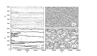
FIG. 1.: Space-time diagram of the active sites in a CML of $500$ sites. Each dot is an active site, i.e. the site with the minimum $x$ at a certain time. $\Delta\lambda=0.1$ in all four cases.(a)$\lambda_{0}=3.7$, $\epsilon=0.5$. (b)$\lambda_{0}=3.9$, $\epsilon=0.5$. (c) $\lambda_{0}=3.8$, $\epsilon=0.1$. (d)$\lambda_{0}=3.9$, $\epsilon=0.1$.

In Fig. 1 we show the space-time picture of the active sites for four different sets of parameters. In all cases we take $g(\lambda)$ uniform within the range $(\lambda_{0},\lambda_{0}+\Delta\lambda)$ and zero outside, with $\Delta\lambda=0.1$. This four cases can be considered paradigmatic of the behaviours observed in a wide region of parameter space. Fig. 1(a) and (b) correspond to a rather high value of the coupling, $\epsilon=0.5$. Fig. 1(c) and (d) have, instead, $\epsilon=0.1$. The value of $\lambda_{0}$ is $3.9$ in (b) and (d), $3.7$ in (a), and $3.8$ in (c). Depending on the value of the parameters, the behaviour of the successive minima can be classified in one of the following four categories.

• discontinuous lines at $i=\mbox{constant}$: The activity is concentrated in a few sites of the system, and in first approximation the same sites remain active as time goes by.

• uniform: The activity is spread all over the system without any apparent order.

• “worms”: The activity is mostly concentrated in a few sites of the system. The activity, however, wanders as time goes by following a random pattern.

• clusterized: The activity is spread all over the system, but in clusters. At variance with (b), at any given time, one sees regions in space where there is no activity.

Let us discuss in more detail Fig. 1(c). The worms are created during the transient. Once created, each worm wanders in space till it encounters a second worm. At that moment they annihilate each other. We have observed that the inactive regions correspond to a periodic pattern in space [30]. The worms, in turn, correspond to defects in the periodicity. Eventually, the last two surviving worms merge, and from there on the activity remains concentrated on a single “fat” worm.

For each one of these cases, we have computed the first return time distribution. This corresponds to the distribution of times between consecutive activity in the same site. We observe that when the successive minima are distributed uniformly in space, the first return time distribution is close to an exponential (see Fig. 2(b)). As soon as the activity is not uniformly distributed, be it lines or irregular clusters, the first return time distribution exhibits a power law decay (asymptotically in case (d)).

To make this picture more quantitative, we present in Fig. 3 a phase diagram, in $\lambda$-$\epsilon$ space ($\Delta\lambda$ is held constant). Phase I is characterised by the presence of power law behaviour in the first return time distribution, $P(\tau)\sim\tau^{-\alpha}$. The value of the exponent of this distribution is not constant within the region. Phase II, on the other hand, is characterised by a non power law behaviour (close to exponential) in the first return time distribution (see Fig. 2(b)). This is tantamount to saying that in phase I there is clusterization of the activity, that is absent in phase II. In Fig. 3 we indicate also a third phase (III), which corresponds to an asymptotic power law (see Fig. 2(d)), with an exponent that is different from that in region I. The border of this region (that we show only schematically) is not as well defined as the border between regions I and II.

FIG. 2.: Distribution of first return time. The parameters correspond to those in Fig. 1: $N=500$, $\Delta\lambda=0.1$, (a)$\lambda_{0}=3.7$, $\epsilon=0.5$. The dashed line corresponds to a power law with exponent $\alpha=1.80(3)$. (b)$\lambda_{0}=3.9$, $\epsilon=0.5$. The dashed line, shown as a reference, corresponds to an exponential decay. (c) $\lambda_{0}=3.8$, $\epsilon=0.1$. The dashed line corresponds to a power law with exponent $\alpha=1.57(2)$. (d)$\lambda_{0}=3.9$, $\epsilon=0.1$. The dashed line corresponds to a power law with exponent $\alpha=1.53(1)$, fitted to the asymptotic region.

This picture holds, qualitatively, even in the absence of the evolutionary dynamics. Indeed, if in every time step we track the position of the minimum, but do not change the value of its $\lambda$ (this corresponds, effectively, to setting $\Delta\lambda=0$), we still obtain the four abovementioned regimes and the corresponding first return time distributions. As $\Delta\lambda$ changes, the value of the exponent in the first return time distribution (in region I) changes as well. Moreover, the area of region II increases with increasing $\Delta\lambda$.

The presence of evolutionary dynamics (i. e. $\Delta\lambda>0$), has yet another effect. The distribution of $\lambda$ evolves in time, from an originally uniform to a stationary non-uniform one. Indeed, this stationary distribution is peaked close to $\lambda_{0}$ and monotonically decresases for larger values of $\lambda$: The system has “self-organized”. Since the extremal dynamics favors higher values of $x$, and the higher the value of $\lambda$ the more likely small values of $x$ are [32], then large values of $\lambda$ are more likely to be updated. The exact shape of this distribution depends on the values of the parameters [33].

Summarizing, the dynamics of extremal coupled maps exhibits a behavior usually associated with criticality:

• First return time distribution is a power law (even in the absence of extremal dynamics)
  

• there is self-organization in the $\lambda$ space
  

• the active regions are localized in space, very much like the avalanches in SOC models (BS).

FIG. 3.: Phase diagram in $\lambda$-$\epsilon$ space. $N=200$, $\Delta\lambda=0.1$. Averaged over 10 realizations.

It is worth emphasizing that this behavior (except the self organization in $\lambda$ space) remains even in the absence of extremal dynamics. In particular, the first return time distribution exhibits a power law behavior. This implies that power law distributions are compatible with non-extremal systems, as has been previously observed by Newman an coworkers [34], in the context of noise-driven systems.

Both SOC and CML models have been used separately in the past to describe evolving ecosystems. To our knowledge, the model presented here is the first synthesis of both ideas that includes the level structure (genotype/phenotype) of real organisms.

REFERENCES

- [1] E-mail: abramson@cab.cnea.gov.ar. Present address: Centro Atómico Bariloche, 8400 Bariloche, Argentina.
- [2] E-mail: jose@mpipks-dresden.mpg.de.
- [3] J.M. Carlson and J.S. Langer, Phys. Rev. Lett. 62, 2632 (1989).
- [4] L. Knopoff and D. Sornette, J. Physique I 5, 1682 (1995).
- [5] S.I. Zaitsev, Physica A 189, 411 (1992).
- [6] A. Petri, G. Paparo, A. Vespignani, A. Alippi and M. Costantini, Phys. Rev. Lett. 73, 3423 (1994).
- [7] P. Diodati, F. Marchesoni and S. Piazza, Phys. Rev. Lett. 67, 2239 (1991).
- [8] G. Caldarelli, F. di Tolla and A. Petri, Phys. Rev. Lett. 77, 2503 (1996).
- [9] D. Wilkinson and J.F. Willemsen, J. Phys. A 16, 3365 (1983).
- [10] M. Cieplak and M.O. Robbins, Phys. Rev. Lett. 60, 2042 (1988).
- [11] K. Sneppen, Phys. Rev. Lett. 69, 3539 (1992).
- [12] K. Sneppen, Phys. Rev. Lett. 71, 101 (1993).
- [13] A. Rinaldo, I. Rodriguez-Iturbe, R. Rigon, E. Ijjasz-Vasquez and R.L. Bras, Phys. Rev. Lett. 70, 822 (1993).
- [14] A. Maritan, F. Colaiori, A. Flammini, M. Cieplak and J.R. Banavar, Science 272, 984 (1996).
- [15] G. Caldarelli, A. Giacometti, A. Maritan, I. Rodriguez-Iturbe and A. Rinaldo, Phys. Rev. E 55, R4865 (1997).
- [16] M.D. Raup, Science 251, 1530 (1986).
- [17] N. Eldredge and S.J. Gould, Punctuated equilibria: an alternative to phyletic gradualism in Models in Paleobiology, Freeman, Cooper and Co., San Francisco (1972).
- [18] S.J. Gould and N. Eldredge, Paleobiology 3, 115 (1977).
- [19] N. Eldredge and S.J. Gould, Nature 332, 211 (1988).
- [20] P. Bak, C. Tang and K. Wiesenfeld, Phys. Rev. Lett. 59, 381 (1987).
- [21] P. Bak, C. Tang and K. Wiesenfeld, Phys. Rev. A 38, 364 (1988).
- [22] M. Paczuski, S. Maslov and P. Bak, Phys. Rev. E 53, 414 (1996).
- [23] P. Bak and K. Sneppen, Phys. Rev. Lett. 71, 4083 (1993).
- [24] P. De Los Rios, A. Valleriani and J. L. Vega, Phys. Rev. E 56, 4876 (1997).
- [25] P. De Los Rios, A. Valleriani and J. L. Vega, Phys. Rev. E 57, 6451 (1998).
- [26] S. Maslov, M. Paczuski and P. Bak, Phys. Rev. Lett. 73, 2162 (1994).
- [27] P. Grassberger, Phys. Lett. A 200, 277 (1995).
- [28] The logistic map is a paradigmatic model of the evolution of in the context of population dynamics. As such, it has been carefully studied and many its properties are well known.
- [29] Coupled Map Lattices have been extensively studied by Kaneko and coworkers [30], as well as many other authors (see [31] and references therein). They exhibit frozen patterns as well as travelling waves depending on the values of and .
- [30] K. Kaneko, Theory and applications of coupled map lattices (John Wiley & Sons, Chichester, 1993).
- [31] H. Chaté and P. Manneville, Prog. Theor. Phys. 87, 1 (1992).
- [32] H. G. Schuster, Determistic Chaos VCH Verlag, Weinheim, 1989).
- [33] This topic is currently under investigation.
- [34] B. W. Roberts and M. E. J. Newman, J. Theor. Biol. 180, 39 (1996).