Evolution dynamics in terraced NK landscapes

Abstract

We consider populations of agents evolving in the fitness landscape of an extended $\bf NK$ model with a tunable amount of neutrality. We study the statistics of the jumps in mean population fitness which occur in the ‘punctuated equilibrium’ regime and show that, for a wide range of landscapes parameters, the number of events in time $t$ is Poisson distributed, with the time parameter replaced by the logarithm of time. This simple log-Poisson statistics likewise describes the number of records in any sequence of $t$ independently generated random numbers. The implications of such behavior for evolution dynamics are discussed.

PACS numbers: 87.10.+e, 87.15.Aa, 05.40.-a

Introduction. Evolutionary dynamics can be described as a stochastic process unfolding in a ‘fitness landscape’[1], a process which can be simulated by means of genetic algorithms [2]. The dynamical behavior of such algorithms is controlled by a number of parameters[3] as e.g. the population size, the rate of mutation and the strenght of selection.

A pervasive dynamical regime is the so-called ‘punctuated equilibrium’[4] or ‘epochal behavior’, where relevant measures of evolution, as e.g. the mean fitness, remain constants for long periods during which the fitness distributions of the individuals is strongly peaked. Occasionally, a fitter mutant appears and quickly ‘takes over’ the population (see e.g. Fig. 1). Real experiments performed on bacterial colonies evolving in a controlled environment have shown that the fitness and cell size increase at a decelerating rate [5]. A similar slowing down is discussed by Kauffman[6] in the ‘long jump’ dynamics of the $\bf NK$ model, while Aranson et al.[7] find a logarithmic growth of the average fitness for quasi-species evolving in a rugged fitness landscape.

In a macroevolutionary context, Raup and Sepkoski[8] suggested that the noticeable decay of the extinction rate[9, 10] might stem from the properties of an underlying optimization process. This idea was taken up in the ‘reset’ model[10, 11], where jumps in the average fitness of populations are linked to fitness record achieved during evolution[12]. Such a link between small and grand scale evolution is rather controversial: If macroevolutionary events are mainly driven extrinsically, e.g. by meteorite impacts[13], any patterns in the fossil record must ultimately stem from the mechanics of celestial bodies in the solar system[14]. Conversely, if, as recently proposed by several authors[15], the fossil record is mainly shaped by complex interactions within the biotic system, macro-evolutionary patterns must emerge from population dynamics.

Our main interest lies in the statistical properties of the evolutionary jumps underlying fitness changes. Since the role of neutral mutations[16] for evolution is well established, and since punctuated equilibria exist even in the absence of local fitness maxima[3, 17], we chose to study evolution on ‘terraced’ landscapes with a tunable degree of neutrality.

We find that, on average, the number of jumps taking place in time $t$ grows proportionate to $\log t$, and that the rate of events consequently decays as $\approx 1/t$. Secondly and most importantly, we show that the record dynamics [10, 12] provides a reasonable description of microevolution, with some limitations which are also outlined. Thirdly, we emphasize that power-law decays generically characterize the correlation functions of time series generated by a record driven dynamics.

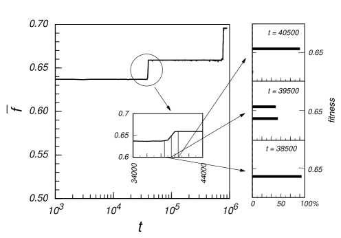
Figure 1: The mean fitness $\overline{f}$ of a single population is shown in the main panel as a function of time. The right panel shows the fitness distributions at times $t=38500$, $t=39500$ and $t=40500$. The simulation parameters are $N=64$, $K=31$, $n=1000$, $\mu_{f}=0.5$, $\sigma_{f}=2.5\times 10^{-3}$, $\beta=1$, $u=10^{-4}$ and $j=10^{9}$, corresponding to the original $\bf NK$ model.

Method. Each ‘genome’ in a population constitutes a point in an abstract configuration space usually called a fitness landscape [1]. To construct such a landscape we use an elegant prescription due to Kauffman, the widely known $\bf NK$ model[18]: We represent genomes as strings of ${\bf N}$ bits ${\bf x}=(x_{1},x_{2},\ldots x_{N})$, each being either $0$ or $1$. The fitness $F(\bf x)$ of configuration $\bf x$ is defined as

$$F({\bf x})=\frac{1}{\bf N}\sum_{i=1}^{\bf N}f_{i},$$ (1)

where the contribution from site $i$, $f_{i}$, is a random function depending on $x_{i}$ and $\bf K$ other $x_{l}$’s. More precisely, $f_{i}$ is a random function of $2^{{\bf K}+1}$ arguments with values uniformly distributed in $(0,1]$. We let $\mu_{f}$ and $\sigma_{f}$ be the average and spread of the distribution from which the $f_{i}$ values are generated.

If $\bf K$ is zero, the change in fitness due to the change of one $x_{i}$ (a point mutation) is of order $1/N$, and the landscape may be regarded as smooth. By way of contrast, when $\bf K={\bf N}-1$ a single point mutation changes all the $f_{i}$’s, and the landscape becomes ‘rugged’. Intermediate cases correspond, of course, to intermediate $\bf K$ values.

Our version of the $\bf NK$ model is modified in two respects. Firstly, the sum in Eq.1 is shifted by $\mu_{f}$ and scaled by $\surd{\bf N}$ rather than $N$. This ensures that the distribution of fitness values keeps the same variance for any value of $N$. More importantly, we introduce tunable neutrality by discretizing the fitness values into ‘terraces’, according to the formula:

$$F^{\prime}({\bf x})=\frac{{\rm nint}(j\surd{\bf N}[F({\bf x})-\mu_{f}]+j\mu_{f})}{j}.$$ (2)

Here $\rm nint$ stands for the nearest integer function, and $j$ denotes the number of terraces. For small $j$ there are few broad terraces, while for $j\rightarrow\infty$ the fitness values approach a continuum and the original $\bf NK$ model is regained. Accordingly, one expects that, as seen e.g. in Fig. 2, the effect of varying $j$ should be stronger for small values of $j$.

In the simulations, a configuration ${\bf x}$ is cloned with a probability $p\propto\exp(\beta F({\bf x}))$. With probability $u<<1$, the cloned string undergoes a one-point mutation at a randomly chosen locus. Finally, a random and fitness independent deletion mechanisms is applied, which keeps the population size fluctuating around a fixed average $n$. Both the generation $/$ mutation part and the deletion part of the algorithm are performed sequentially. Subsequently, the information about the new fitness distribution is incorporated in the cloning probabilities. This entire process counts as one update and defines the unit of time.

Punctuated equilibrium dynamics requires that a fitter mutant be able to survive and spread in the population on a time scale short compared to the inverse mutation frequency. Therefore, $u$ should not be too high and $\beta$ should not be too low. Within these constraints $u$ should be as high as possible, in order to have a good statistics within the time window of the computation. Also, too high a $\beta$ value quenches the dynamics completely. These design consideration lead to the values of $u$ and $\beta$ used throughout the calculations.

A concise description of the dynamics is provided by the average $\overline{f}(t)$ of the distribution of fitness values through the population. Such a trajectory is shown in the main panel of Fig. 1 to consist of a number of flat plateaus separated by rather well defined jumps. The number $m(t)$ of jumps occurring in the interval $[0,t)$ is a stochastic process whose distribution can be sampled by repeating the simulations or, equivalently, by considering an ensemble of landscapes, where different trajectories are generated by independently updating each system. The ensemble average and variance of $m$ are denoted by $E(m)$ and $\sigma^{2}(m)$ respectively, while $a_{m}(t)$ and $v_{m}(t)$ are the corresponding estimators. The notation describing the inputs and results of our simulations is summarized in Table 1.

variable	meaning	values
$\bf N$	genome length	$64$
${\bf K}$	degree of ruggedness	$7,15$ and $31$
$n$	population size	$1000$
$\sigma_{f}$	spread of $f_{i}$’s in Eq.1	$2.5\times 10^{-3}$
$\mu_{f}$	mean of $f_{i}$’s in Eq.1	$0.5$
$j$	number of terraces	$10$ - $10^{9}\approx\infty$
$\beta$	reproductive selectivity	$1$
$u$	mutation prob. per cloning	$10^{-4}-5\cdot 10^{-4}$
$s$	ensemble size	$s=80$
$\overline{f}$	population averaged fitness	see Fig. 1
$m$	no. of evol. steps	see Fig. 2
$a_{m}(t)$	sample average of $m$	-
$\lambda$	$\lambda\log t\approx a_{m}(t)$	see slopes of Figs. 2 and 3

Table 1: The table summarizes the notation and parameter valuse used in the text.

Results. The basic qualitative features of the data are expressed by Fig. 1: Its left panel shows the mean fitness $\overline{f}$ of a single population on a semilogarithmic scale. The right panel details the behavior close to the evolutionary jump at $t\approx 3\times 10^{4}$ by depicting the distribution of fitness values right before, during and right after the jump. Nearly all strings have the same fitness in the initial and final situations, while the transition stage features two different fitness values. Punctuated equilibrium behavior and a very peaked fitness distribution are widely found in previous studies[19, 20] as well as in our simulations.

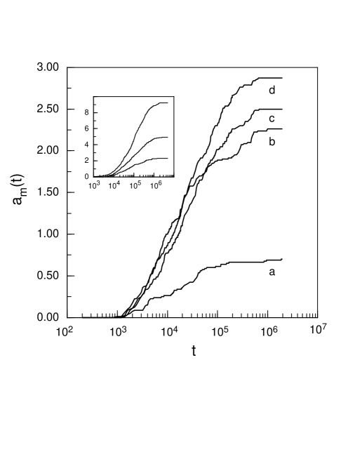
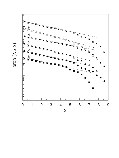
Figure 2: Sample average of the number of fitness jumps, $a_{m}$ as a function of time $t$ for landscapes with ${\bf K}=31$ and $a:j=10$, $b:j=10^{2}$, $c:j=10^{3}$ and $d:j=10^{9}$. The mutation rate is $u=5\times 10^{-4}$. The insert shows the same quantity, but for landscapes with no terraces ($j=10^{9}$) and with ${\bf K}=7$ (top curve), ${\bf K}=15$ and ${\bf K}=31$ (bottom curve). The mutation rate is here $u=10^{-4}$.

Figure 3: Distribution of log-waiting times for landscapes with ${\bf K}=31$ and $a:j=10^{2}$, $b:j=10^{3}$, $c:j=10^{4}$, $d:j=10^{5}$, $e:j=10^{6}$ and $f:j=10^{9}$. For graphical clarity the curves are vertically shifted relative to each other by a factor of four. The mutation rate is $u=5\times 10^{-4}$.

For a more quantitative data analysis, the statistical properties of the jumps and their associated waiting times must be studied. We let $m_{i}(t)$ be the number of jumps occurred at time $t$ in trajectory $i$, and consider the sample average:

$$a_{m}(t)=\frac{\sum_{i=1}^{s}m_{i}(t)}{s},$$ (3)

and the sample variance:

$$v_{m}(t)=\frac{\sum_{i=1}^{s}(m_{i}(t)-a_{m}(t))^{2}}{s-1}$$ (4)

as functions of time. To calculate error bars on $a_{m}$ and $v_{m}$ we need the corresponding standard deviations, which are $\sigma(m)/\surd s$ and $\surd(\sigma^{2}(m^{2})+8E^{2}(m)E(m^{2})-4E(m)(E^{3}(m)+E(m^{3})))/\surd s+{\cal O}(1/s)$. The latter relation results from straightforward but rather tedious algebra. To lowest order in $s^{-1/2}$ one may now replace the moments of $m$ with their sample estimators. In general, the relative errors on various quantities of interest are of order $1/\surd s\approx 10\%$.

Fig. 2 shows the average number of jumps, for a number of different parameters values, as a function of time. $E(m)$ is seen to grow logarithmically, with a strong ${\bf K}$ dependence slope, for ‘short’ log-times. The leveling off noticed at large times stems from the fact that, as the fitness increases, fitness improvements become progressively smaller. Eventually, they get lost in the noise, rather than triggering a jump. At this point record statistics and fitness evolution must part company.

For large $t$, the probability of $n$ records in a sequence of $t$ independently drawn random numbers is given by[21]:

$$P_{t}(n)=\frac{(\log\lambda t)^{n}}{n!}t^{-\lambda}.$$ (5)

This is a Poisson distribution with $\log t$ replacing the time argument. The strength parameter $\lambda$ describes the possibility that many searches for records take place independently and in parallel and/or the situation where records remain undetected. In our systems we observed that several records were indeed lost in the noise, and did not trigger any evolutionary event.

A mathematically equivalent description of record dynamics is provided by the distribution of the variables

$$\Delta_{k}=\log t_{k}-\log t_{k-1}=\log(t_{k}/t_{k-1}).$$ (6)

It follows from standard arguments that in a (log) Poisson process these $\Delta_{k}$ are independent and have the common distribution:

$$P(\Delta>x)=\exp(-\lambda x).$$ (7)

The empirical distribution of the $\Delta_{k}$’s is shown on a semilogarithmic scale in Fig. 3 for ${\bf K}=31$ and for differing degrees of terracing. The decay of $P(\Delta>x)$ seems quite well described by an exponential for $x\leq 5$, with the tail of the distribution falling off more rapidly, likely due to the inevitably poor sampling of large $x$ values in a finite time simulation. Banning the effect of the deviations from pure record statistics, $\lambda$ is, by Eqs. 5 and 7, the slope of $a_{m}(t)$ vs. $\log t$ as well as minus the slope of $\log P(\Delta>x)$ vs $x$. We calculated these slopes from the data in both ways (cutting off the tails of the data), and obtained the following results. $j=10^{2},\;\lambda=0.54\;(0.34)$; $j=10^{3},\;\lambda=0.49\;(0.39)$; $j=10^{4},\;\lambda=0.58\;(0.44)$; $j=10^{5},\;\lambda=0.54\;(0.35)$; $j=10^{6},\;\lambda=0.62\;(0.47)$; and $j=10^{9},\;\lambda=0.63\;(0.39)$. The figures in parentheses stem from Fig. 3. There is a rough agreement, but certainly also considerable scatter in these data, with the log-wait time type of analysis yielding systematically lower figures. At this stage it is unclear whether the non-monotonic dependence of $\lambda$ on $j$ seen in Fig. 3 is a real effect - or just due to a combination of statistical fluctuations and systematic deviations from the ideal log-Poisson behavior.

Summarizing the results from Figs. 2 and 3, it appears that the value of ${\bf K}$ very strongly affects the average slope of the curves (i.e. the value of $\lambda$). The degree of terracing might also have an effect on the slope, albeit a minor one.

The independence of the different $\Delta_{k}$’s implied by the record statistics was tested by calculating the correlation coefficients $C_{ij}$ between $\Delta_{i}$ and $\Delta_{j}$. In practice, we checked for $C_{12}$, $C_{23}$ and $C_{13}$. As expected, the highest degree of correlation was found for the relatively smooth landscape with ${\bf K}=7$. In this case, the $C$ values were close to $0.4$. For ${\bf K}=31$ the correlation coefficients were of the order of $0.1$, i.e. of the same order as the statistical sampling error.

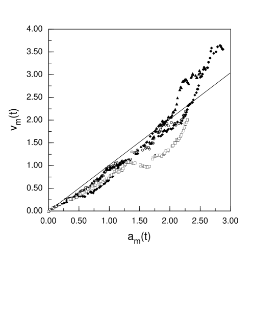
Figure 4: Sample variance, $v_{m}$, of the number of fitness jumps versus sample average, $a_{m}$, of the same quantity. The data are all for ${\bf K}=31$. Squares and filled diamonds are both for for unterraced landscapes ($j=10^{9}$), and have mutation rates $u=10^{-4}$ and $u=5\cdot 10^{-4}$ respectively. The other two data sets both have $u=5\cdot 10^{-4}$. The degree of terracing is $j=10^{2}$ (circles) and $j=10^{3}$ (filled triangles).

To conclude the description of our data we plot in Fig. 4 the estimated variance $v_{m}(t)$ versus the estimated average $a_{m}$, for ${\bf K}=31$ and a number of terrace values. For a perfect agreement with the log-Poisson distribution the points should lie on a straight line of slope $1$. This is close to the observed behavior, except for the highest values (where, on the other hand, the statistics is poorest). A similar plot for ${\bf K}=15$ and ${\bf K}=7$ shows a systematic deviation from a straight line, with considerably less variance than in a purely random case. Additional details on the simulations and on the genetic algorithm utilized to produce them can be found in Ref. [22].

In summary, the dynamics of our evolutionary model is time inhomogeneous stochastic process, with a rate of events falling off as $1/t$. The log-Poisson statistics describes the data best for landscapes with large $\bf K$, with or without terraces. In this respect terraces have a minor effect on the dynamics.

Discussion. While the shape of the fossil record certainly reflects many different factors[15], including e.g. biogeography[23] and external perturbations of the abiotic environment[13], the event statistics demonstrated here should have rather general implications for all models which do not completely dismiss the influence of population dynamics on macroevolution. If the evolutionary ‘jumps’ are the elementary events in any dynamics, possibly involving interactions between evolving species, using $\log t$ as the independent variable makes this dynamics appear as a stationary, markovian process, described e.g. by a master or Fokker-Planck equation. The eigenvalues (and eigenvectors) of the evolution equation describe the relaxation of any average of interest. Since the observational time window is usually narrow in $\log$ time, one is restricted to observing the decay of a single (or a few) relaxational mode(s). As an exponential function of $\log$ is a power-law, the above mechanism offers a generic explanation for the power-law like behavior found in several evolutionary patterns.

Aknowledgments. Both authors would like to thank Mark Newman and Richard Palmer for inspiring conversations and exchanges of ideas at the Santa Fe Institute of Complex Studies and at the Telluride Summer Research Institute. Parts of this work were commenced during a visit by A. P. at Duke University. A. P. owes a special thank to Richard Palmer for the kind hospitality extended to him and for the guidance he received during his stay. This project was partly supported by a block grant from Statens Naturvidenskabelige Forskningsråd.

References

- [1] S. Wright Genetics 16, 97 (1931)
- [2] J. H. Holland Adaptation in Natural and Artificial Systems. U. of Michigan Press. (1975)
- [3] E. van Nimwegen, J. P. Crutchfield and M. Mitchell Phys. Lett., A 229, 144 (1997)
- [4] N. Eldredge and S. J. Gould Punctuated equilibria: An alternative to phyletic gradualism Models in Paleobiology. (T. J. M. Schopf, ed.). Freeman, Cooper, San Francisco (1972)
- [5] Richard E. Lenski and Michael Travisano Proc. Natl. Acad. Sci. USA, 91, 6808 (1994), and Dynamics of adaptation and diversification, in Tempo and mode in evolution, Walter M. Fitch and Francisco J. Ayala Ed., National Academy of Sciences (1995)
- [6] Stuart Kauffman At home in the universe, Chapt. 9, Oxford University Press (1995)
- [7] I. Aranson, L. Tsimring and V. Vinokur Phys. Rev. Lett., 79, 3298 (1997)
- [8] David M. Raup and J. J. Sepkoski, Jr. Science, 215, 1501 (1982)
- [9] M. E. J. Newman and Gunther J. Eble, Paleobiology, 25, 434, (1999)
- [10] Paolo Sibani, Michel R. Schmidt and Preben Alstrøm Phys. Rev. Lett., 75, 2055 (1995)
- [11] Paolo Sibani Phys. Rev. Lett., 79, 1413 (1997)
- [12] Preben Alstrøm europhysics news, 30, 22 (1999)
- [13] Luis W. Alvarez, Walter Alvarez, Frank Asaro and Helen V. Michel Science 208, 1095 (1980)
- [14] D. M. Raup and J. J. Sepkoski, Jr. Proc. Natl. Acad. Sci. USA 81, 801 (1984)
- [15] M. E. J. Newman and R. G. Palmer www.santafe.edu/mark/pubs.html Models of extinction: a review. See also: Paolo Sibani, Michael Brandt and Preben Alstrøm Int. J. Mod. Phys., B 12, 361, (1998)
- [16] M. Kimura. The neutral theory of molecular evolution Cambridge University Press 1983.
- [17] Stefan Bornholt and Kim Sneppen Phys. Rev. Lett., 81, 236 (1998)
- [18] S. A. Kauffman and S. Levine J. Theor. Biol., 128, 11 (1987)
- [19] G. Weisbuch, in Spin glasses and biology, edited by D. L. Stein (World Scientific, Singapore, 1992), pp. 141–158
- [20] M. E. J. Newman and Robin Engelhardt Proc. R. Soc. London, B 265, 1333, (1998)
- [21] Paolo Sibani and Peter B. Littlewood Phys. Rev. Lett., 71, 1485 (1993)
- [22] Andreas Pedersen Master Thesis: Evolutionary Dynamics, Odense Universitet, (1999), see: http://planck.fys.ou.dk/ap/Public/thesis.ps
- [23] Jon D. Pelletier Phys. Rev. Lett., 82, 1983 (1999)