Time evolution of averages
in dynamical systems driven by noise

Abstract

This paper presents description of time evolution of averages of Markov process in wide range of noise intensity. Exact expression of time scale of average evolution has been obtained. It has been demonstrated numerically that for purely noise-induced transitions (transitions over potential barriers) the time evolution of mean coordinate is a simple exponent with a good precision even for the case when the potential barrier height is comparable or smaller than the noise intensity. Also it has been demonstrated that nonlinear system may be ”linearized” by a strong noise.

PACS numbers: 05.40.+j
Keywords: Brownian motion, Markov process, time evolution of averages.

I Introduction

Overdamped Brownian motion in a field of force (Markov process with nonlinear drift coefficient) is a model widely used for description of noise-induced transitions in different polystable systems. Values that may be observed in experiment are different averages and knowledge of their time evolution is a subject of great theoretical and practical importance in a wide variety of tasks (e.g. tasks of Josephson electronics [1], stochastic resonance [2], ratchet effect [3],[4], and so on).

In paper by Nadler and Schulten [5] the authors have demonstrated exponential behavior of observables for relaxation processes in systems having steady states. Namely, using the approach of ”generalized moment approximation” the authors of [5] obtained some exact characteristic time scales and for particular example of a rectangular potential well demonstrated good coincidence of exponential approximation with numerically obtained observables.

In the frame of this paper we consider time evolution of averages of an overdamped Brownian motion. Extending the approach by Malakhov we have obtained exact characteristic scales of time evolution of averages (valid for arbitrary potentials and noise intensity). Some particular examples of time evolution of mean coordinate of overdamped Brownian motion in monostable and bistable potentials have been considered. It has been demonstrated that time behavior of mean coordinate is very well approximated by the exponent for purely noise-induced transitions (transitions over potential barriers) even in the case of a large noise intensity in comparison with potential barrier height. Also, an effect of ”linearization” of nonlinear systems by a strong noise has been observed.

It is necessary to mention that in difference from approach used in [5], our approach allows to describe time evolution of averages for tasks with arbitrary boundary conditions, e.g. the case of periodic boundary conditions $\varphi(\pi)=\varphi(-\pi)$ as application to tasks of Josephson electronics will be soon presented elsewhere. Moreover, as it seems now, the use of the presented approach for description of ratchet effect may allow to get the required optimal frequency of flashing [3] for periodic potentials of arbitrary shape.

II Main equations and set up of the problem

Consider a process of Brownian diffusion in a potential profile ${\mit\Phi(x)}$. Let a coordinate $x(t)$ of the Brownian particle described by the probability density $W(x,t)$ at initial instant of time has a fixed value $x(0)=x_{0}$, i.e. the initial probability density is the delta function:

$$W(x,0)=\delta(x-x_{0}).$$ (1)

It is known that the probability density $W(x,t)$ of the Brownian particle in the overdamped limit (Markov process) satisfies to the Fokker–Planck equation (FPE):

$${\partial W(x,t)\over\partial t}=-{\partial G(x,t)\over\partial x}={1\over B}\left\{{\partial\over\partial x}\left[{d\varphi(x)\over dx}W(x,t)\right]+{\partial^{2}W(x,t)\over\partial x^{2}}\right\}.$$ (2)

Here $B=\displaystyle{h/{kT}}$, $G(x,t)$ is the probability current, $h$ is the viscosity (in computer simulations we put $h=1$), $T$ is the temperature, $k$ is the Boltzmann constant and $\varphi(x)=\displaystyle{\mit\Phi(x)/kT}$ is the dimensionless potential profile. In this paper we will only consider an overdamped Brownian motion in potentials $\varphi(x)$ such that ${\varphi(\pm\infty)}=+\infty$, i.e. eventually the probability density will reach a steady-state $W_{st}(x)=Ae^{-\varphi(x)}\neq 0$ ($A=1/\int\limits_{-\infty}^{+\infty}e^{-\varphi(x)}dx$). This leads to the following boundary conditions: $G(\pm\infty,t)=0$. Besides, the growth of the walls of the potential $\varphi(x)$ should be fast enough for applicability of the method described below (for $\varphi(x)\sim x^{n}$, where $n\leq 1$, the method not always gives correct results).

We will search for the average $m_{f}(t)$ in the form:

$$m_{f}(t)=<f(x)>=\int\limits_{-\infty}^{+\infty}f(x)W(x,t)dx.$$ (3)

Let us mention that the approach we use may be easily extended for description of time evolution of some kind of conditional averages when the limits $\pm\infty$ may be substituted by arbitrary interval $(c,d)$, such that boundary conditions at $c$ and $d$ are arbitrary.

Following this obvious definition (3) it is necessary to know the solution of the FPE - the probability density $W(x,t)$ - for obtaining the required average. But the nonstationary solution of FPE is unknown in general case of nonlinear systems. However, as it has been demonstrated recently in [6],[7], the time evolution of the probability $P(t)=\int\limits_{c}^{d}W(x,t)dx$ may be very well (with only few percent mistake) approximated by the exponent even when the noise intensity is larger than a potential barrier height. Besides, it is well-known that the time evolution of mean coordinate of Brownian motion in a parabolic potential (linear system) is exactly exponential. This allows to hope that time evolution of different averages of Markov process may be in many cases very well described by exponential approximation in wide range of noise intensity.

Modifying the approach by Malakhov [8],[9], it is possible to define some characteristic scale of time evolution of the required average (similar way was used in [5]) and obtain exact analytic expression for this time scale. After that, substituting the obtained time scale into the factor of exponent and comparing the obtained time evolution of the average with computer simulation results we will test applicability of this approximation for different types of potentials in wide range of noise intensity.

III Characteristic time scale of evolution of average of Markov process

Let us consider attentively the FPE (2). This is a continuity equation:

$${\partial W(x,t)\over\partial t}=-{\partial G(x,t)\over\partial x}.$$ (4)

To obtain necessary average $m_{f}(t)$ (3) let us multiply equation (4) by the function $f(x)$ and integrate it with respect to $x$ from $-\infty$ to $+\infty$. Then we get:

$${dm_{f}(t)\over dt}=-{\int\limits_{-\infty}^{+\infty}f(x)dG(x,t)}.$$ (5)

This is already ordinary differential equation of the first order ($f(x)$ is known deterministic function), but nobody knows how to find $G(x,t)$.

Let us define the characteristic scale of time evolution of the average $m_{f}(t)$ by similar way as it was done for time scale of the probability evolution in [8],[9]:

$$\tau_{f}(x_{0})={\int\limits_{0}^{\infty}\left[m_{f}(t)-m_{f}(\infty)\right]dt\over m_{f}(0)-m_{f}(\infty)}.$$ (6)

Definition (6) is general in the sense that it is valid for any initial condition. But in the frame of this paper we restrict ourselves by the delta-shaped initial distribution (1) and consider $\tau_{f}(x_{0})$ as function of $x_{0}$. For arbitrary initial distribution the required time scale may be obtained from $\tau_{f}(x_{0})$ by simple averaging over initial distribution. If the required function $m_{f}(t)$ evolves exponentially in time $m_{f}(t)\sim e^{-t/\tau}$ then the time scale $\tau$ in the factor of exponent coincides with $\tau_{f}(x_{0})$ defined by (6).

It is necessary to mention that definition (6) gives correct results only for monotonically evolving functions $m_{f}(t)$. Besides, $m_{f}(t)$ should fast enough approach its steady-state value $m_{f}(\infty)$ for convergence of the integral in (6).

The required evolution time of the average $m_{f}(t)$ may be obtained via the approach proposed by Malakhov [8],[9]. This approach is based on the Laplace transformation method $m_{f}(s)=\int\limits_{0}^{\infty}m_{f}(t)e^{-st}dt$. We will only slightly modify this approach with respect to our task.

Performing Laplace transform of formula (6), Eq. (5) (Laplace transformation of (5) gives: $sm_{f}(s)-m_{f}(0)=-\int\limits_{-\infty}^{+\infty}f(x)d\hat{G}(x,s)$) and combining them, we get:

$$\tau_{f}(x_{0})=\lim_{s\to 0}{sm_{f}(s)-m_{f}(\infty)\over s[m_{f}(0)-m_{f}(\infty)]}=\lim_{s\to 0}{m_{f}(0)-m_{f}(\infty)-\int\limits_{-\infty}^{+\infty}f(x)d\hat{G}(x,s)\over s[m_{f}(0)-m_{f}(\infty)]}.$$ (7)

where $\hat{G}(x,s$) is the Laplace transformation of the probability current $\hat{G}(x,s)=\int\limits_{0}^{\infty}G(x,t)e^{-st}dt$.

Following the approach by Malakhov, one can introduce the function $H(x,s)\equiv s\hat{G}(x,s)$, and expand it in the power series in $s$:

$$H(x,s)\equiv s\hat{G}(x,s)=H_{0}(x)+sH_{1}(x)+s^{2}H_{2}(x)+\ldots$$ (8)

It is possible to find the differential equations for $H_{n}(x)$ (see [9]):

$$\begin{array}[]{ll}\displaystyle{\frac{dH_{1}(x)}{{dx}}}=-W_{st}(x)+\delta(x-x_{0}),&\\ \displaystyle{\frac{d^{2}H_{n}(x)}{{dx^{2}}}}+{\frac{d\varphi(x)}{{dx}}}{\frac{dH_{n}(x)}{{dx}}}=BH_{n-1}(x),\quad n=2,3,4,\ldots\end{array}$$ (9)

Here $W_{st}=Ae^{-\varphi(x)}$, $A=1/\int\limits_{-\infty}^{+\infty}e^{-\varphi(x)}dx$. Using the natural boundary conditions $G(\pm\infty,t)=0$, one can obtain from (9) $H_{1}(x)=-A\int\limits_{-\infty}^{x}e^{-\varphi(v)}dv+1(x-x_{0})$ and

$$H_{2}(x)=B\left\{\int\limits_{-\infty}^{x}e^{-\varphi(v)}\int\limits_{-\infty}^{v}e^{\varphi(y)}[1(y-x_{0})-F(y)]dydv-\right.$$ (10)

$$\left.-F(x)\int\limits_{-\infty}^{+\infty}e^{-\varphi(v)}\int\limits_{-\infty}^{v}e^{\varphi(y)}[1(y-x_{0})-F(y)]dydv\right\},$$ (11)

where

$$F(u)=\int\limits_{-\infty}^{u}e^{-\varphi(v)}dv/\int\limits_{-\infty}^{+\infty}e^{-\varphi(v)}dv.$$ (12)

Here we restricted ourselves by obtaining of $H_{2}(x)$ only, because substituting the set (8) into formula (7) one can get:

$$\tau_{f}(x_{0})=-{\int\limits_{-\infty}^{+\infty}f(x)dH_{2}(x)\over[m_{f}(0)-m_{f}(\infty)]}.$$ (13)

Thus, substituting $H_{2}(x)$ (11) into formula (13) one can get the characteristic scale of time evolution of any average $m_{f}(t)$ for arbitrary potential such that $\varphi({\pm\infty})=\infty$:

$$\tau_{f}(x_{0})=\frac{B}{m_{f}(0)-m_{f}(\infty)}\times$$ (14)

$$\times\left\{\int\limits_{-\infty}^{\infty}f(x)e^{-\varphi(x)}\int\limits_{x_{0}}^{x}e^{\varphi(u)}F(u)dudx-A\int\limits_{-\infty}^{\infty}f(x)e^{-\varphi(x)}dx\int\limits_{-\infty}^{\infty}e^{-\varphi(x)}\int\limits_{x_{0}}^{x}e^{\varphi(u)}F(u)dudx+\right.$$ (15)

$$\left.+A\int\limits_{-\infty}^{\infty}f(x)e^{-\varphi(x)}dx\int\limits_{x_{0}}^{\infty}e^{-\varphi(x)}\int\limits_{x_{0}}^{x}e^{\varphi(u)}dudx-\int\limits_{x_{0}}^{\infty}f(x)e^{-\varphi(x)}\int\limits_{x_{0}}^{x}e^{\varphi(u)}dudx\right\},$$ (16)

where $F(x)$ is expressed by (12) and $A=1/\int\limits_{-\infty}^{+\infty}e^{-\varphi(x)}dx$.

Once we know the required time scale of the evolution of average, we can present the required average in the form:

$$m_{f}(t)=(m_{f}(0)-m_{f}(\infty))\exp(-t/\tau_{f}(x_{0}))+m_{f}(\infty).$$ (17)

The applicability of this formula for several examples of time evolution of mean coordinate $m(t)=<x(t)>$ will be checked in the next section.

IV Time evolution of mean coordinate of Markov process

As an example of description presented above, let us consider time evolution of mean coordinate of Markov process:

$$m(t)=<x(t)>=\int\limits_{-\infty}^{+\infty}xW(x,t)dx.$$ (18)

The characteristic time scale of evolution of the mean coordinate in general case may be easily obtained from (15) substituting $x$ for $f(x)$. But for symmetric potentials $\varphi(x)=\varphi(-x)$ the expression of time scale of mean coordinate evolution may be significantly simplified ($m(\infty)=0$):

$$\tau_{m}(x_{0})=\frac{B}{x_{0}}\left\{\int\limits_{0}^{+\infty}xe^{-\varphi(x)}dx\cdot\int\limits_{0}^{x_{0}}e^{\varphi(u)}du+\int\limits_{0}^{x_{0}}xe^{-\varphi(x)}\int\limits_{x_{0}}^{x}e^{\varphi(u)}dudx\right\}.$$ (19)

If $x_{0}=0$ then, as not difficult to check, $\tau_{m}(x_{0})=0$.

Let us consider now some examples of symmetric potentials and check applicability of exponential approximation:

$$m(t)=<x(t)>=x_{0}\exp(-t/\tau_{m}(x_{0})).$$ (20)

First we should consider time evolution of mean coordinate in monostable parabolic potential $\varphi(x)=ax^{2}/2$ (linear system), because for this case time evolution of mean is known:

$$m_{par}(t)=x_{0}\exp(-at/B),$$ (21)

where $a=a^{\prime}/kT$ and $B=h/kT$, so $\tau_{par}=B/a$ for linear system and does not depend on noise intensity and the coordinate of initial distribution $x_{0}$. On the other hand, $\tau_{m}(x_{0})$ is expressed by formula (19). Substituting parabolic potential $\varphi(x)=ax^{2}/2$ in formula (19), making simple substitutions and changing order of integrals, it can be easily demonstrated that $\tau_{m}(x_{0})=B/a=h/a^{\prime}=\tau_{par}$, so for purely parabolic potential the time of mean evolution (19) is independent of both noise intensity and $x_{0}$ as it must. This fact proves the correctness of the used approach.

The second considered example is described by the monostable potential of the fourth order: $\varphi(x)=ax^{4}/4$. In this nonlinear case the applicability of exponential approximation significantly depends on the location of initial distribution and the noise intensity. Nevertheless, the exponential approximation of time evolution of the mean gives qualitatively correct results and may be used as first estimation in wide range of noise intensity (see Fig. 1, $a=1$). Moreover, if we will increase noise intensity further, we will see, that error of our approximation decreases and for $kT=50$ we get that the exponential approximation and the results of computer simulation coincide (see Fig. 2, plotted in the logarithmic scale, $a=1$, $x_{0}=3$). From this plot we can conclude that nonlinear system is ”linearized” by strong noise - effect which is qualitatively obvious, but should be investigated further by the analysis of variance and higher cumulants.

The third considered example is described by the bistable potential - the so-called ”quartic” potential: $\varphi(x)=ax^{4}/4-bx^{2}/2$. In this case the applicability of exponential approximation also significantly depends on the coordinate of initial distribution. If $x_{0}$ is far from the potential minimum, then there exists two characteristic time scales: fast dynamic transition to potential minimum and slow noise-induced escape over potential barrier. In this case exponential approximation gives not so adequate description of temporal dynamics of the mean, however may be used as first estimation. But if $x_{0}$ coincide with the potential minimum, then the exponential approximation of the mean coordinate only few percent differs from results of computer simulation even in the case when noise intensity is significantly larger than the potential barrier height (strongly nonequilibrium case) (see Fig. 3, $a=1$, $b=2$, $x_{0}=1.414$). If, however, we consider the case when the initial distribution $x_{0}$ is far from the potential minimum, but the noise intensity is large, we will see again as in previous example that essential nonlinearity of the potential is suppressed by strong fluctuations and the evolution of the mean coordinate becomes exponential (see Fig. 4, plotted in the logarithmic scale, $a=1$, $b=2$, $x_{0}=2.5$).

V Conclusion

In the frame of this paper we have considered time evolution of averages of an overdamped Brownian motion. Extending the approach by Malakhov we have obtained exact characteristic scales of time evolution of averages (valid for arbitrary potentials and noise intensity). Some particular examples of time evolution of mean coordinate of overdamped Brownian motion in monostable and bistable potentials have been analyzed.

It has been demonstrated that for purely noise-induced transitions (transitions over potential barriers) the time evolution of mean coordinate is a simple exponent with a good precision even for the case when the potential barrier height is comparable or smaller than the noise intensity.

Also, there has been observed the effect of ”linearization” of nonlinear system by a strong noise in the sense that time evolution of mean coordinate becomes purely exponential with increase of noise intensity.

VI Acknowledgments

Author wishes to thank Prof. A.N.Malakhov for attentive reading of the manuscript and constructive comments, and Prof. V.N.Belykh for helpful discussions.

This work has been supported by the Russian Foundation for Basic Research (Project N 96-02-16772-a, Project N 96-15-96718 and Project N 97-02-16928), by Ministry of High Education of Russian Federation (Project N 3877) and in part by Grant N 98-2-13 from the International Center for Advanced Studies in Nizhny Novgorod.

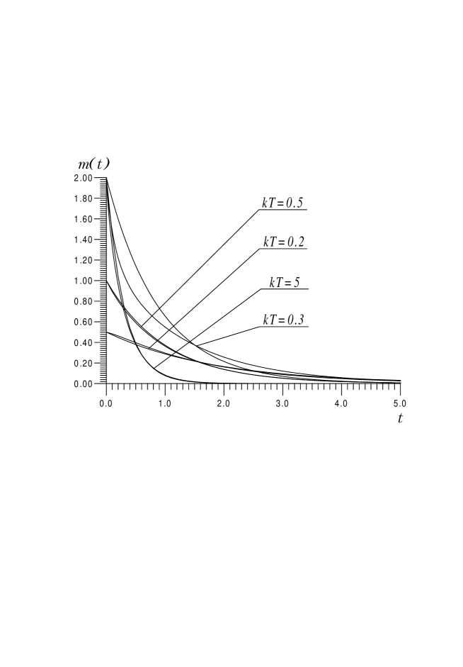
FIG. 1.: Evolution of the mean coordinate in the potential ${\mit\Phi(x)}=x^{4}/4$ for different values of noise intensity.

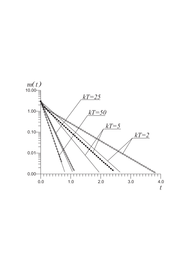
FIG. 2.: Evolution of the mean coordinate in the potential ${\mit\Phi(x)}=x^{4}/4$ for different values of noise intensity.

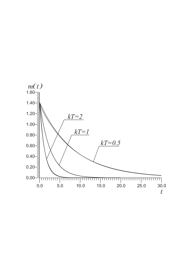
FIG. 3.: Evolution of the mean coordinate in the potential ${\mit\Phi(x)}=x^{4}/4-x^{2}$ for different values of noise intensity with initial distribution located in a potential minimum.

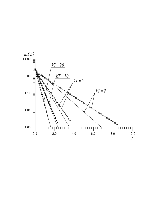
FIG. 4.: Evolution of the mean coordinate in the potential ${\mit\Phi(x)}=x^{4}/4-x^{2}$ for different values of noise intensity with initial distribution located far from a potential minimum.

REFERENCES

- [1] K.K. Likharev, Dynamics of Josephson Junctions and Circuits (Gordon and Breach, New York, 1986).
- [2] L.Gammaitoni, P.Hanggi, P.Jung and F.Marchesoni, Rev. Mod. Phys., 70 (1998) 223.
- [3] F.Julicher, A.Ajdari and J.Prost, Rev. Mod. Phys, 69 (1997) 1269.
- [4] C.R.Doering, Physica A, 254 (1998) 1.
- [5] W.Nadler and K.Schulten, Journ. Chem. Phys., 82 (1985) 151.
- [6] S.P.Nikitenkova and A.L.Pankratov, Physical Review E, in press (will appear in the issue of December 1, 1998).
- [7] S.P.Nikitenkova and A.L.Pankratov, Preprint N adap-org/9807001 at http://xxx.lanl.gov.
- [8] A.N.Malakhov and A.L.Pankratov, Physica C, 269 (1996) 46.
- [9] A.N.Malakhov, CHAOS, 7 (1997) 488.