Critical Exponent of Species-Size Distribution in Evolution

Abstract

We analyze the geometry of the species– and genotype-size distribution in evolving and adapting populations of single-stranded self-replicating genomes: here programs in the Avida world. We find that a scale-free distribution (power law) emerges in complex landscapes that achieve a separation of two fundamental time scales: the relaxation time (time for population to return to equilibrium after a perturbation) and the time between mutations that produce fitter genotypes. The latter can be dialed by changing the mutation rate. In the scaling regime, we determine the critical exponent of the distribution of sizes and strengths of avalanches in a system without coevolution, described by first-order phase transitions in single finite niches.

Introduction

Power law distributions in Nature usually signal the absence of a scale in the region where the scaling is observed, and sometimes point to critical dynamics. In Self-Organized-Criticality (SOC) (Bak, Tang, and Wiesenfeld 1987, 1988), for example, power law distributions reveal the dynamics of an unstable critical point, brought about by slow driving and a feed-back mechanism between order parameter and critical parameter. The critical dynamics is usually described within the language of second-order phase transitions in condensed matter systems (Sornette, Johansen and Dornic 1996), but it can be shown that SOC-type behavior also occurs within a dual description in terms of the Landau-Ginzburg equation as first-order transitions (Gil and Sornette 1996). Indeed, it was shown that a power law distribution of epoch-lengths, that is, the time a particular species dominates the dynamics of an adapting population, is explained by a self-organized critical scenario (Adami 1995) that carries the hallmark of first-order phase transitions. Here, we measure the distribution of abundances of species and genotypes in an artificial chemistry, (the Avida Artificial Life system, Adami and Brown 1995, Ofria, Brown and Adami 1998) and show that the distribution is scale-free under a broad class of circumstances, confirming the results reported in Adami (1995). In the next section, we discuss the first-order dynamics in more detail and examine “avalanches of invention” from the point of view of a thermodynamics of information. In Section III, we measure the critical exponent of the power law of genotype abundances in the limit of infinitesimal driving, i.e., infinitesimal mutation rate, and discuss the role of the fitness landscape in shaping the distribution. In Section IV, we repeat the analysis for a higher taxonomic level (that of species) and discuss its relation to the geometric distributions found by Burlando (1990, 1993). Conclusions about the evolutionary process drawn from the data obtained in this paper are presented in Section V.

Self-Organization in Evolution

The idea that the evolutionary process occurs in spurts, jumps, and bursts rather than gradual, slow and continuous changes has been around for over 75 years (Willis 1922), but has gained prominence as “punctuated equilibrium” through the work of Gould and Eldredge (1977, 1993). The general idea is that evolutionary innovations are not bestowed upon an existing species as a whole, gradually, but rather by the emergence of one better adapted mutant which, by its superiority, serves as the seed of a new breed that sweeps through an ecological niche and supplants the species previously occupying it. The global dynamics thus has a microscopic origin, as shown experimentally, e.g., in populations of E. Coli by Elena, Cooper and Lenski (1996).

Such avalanches can be viewed in two apparently contradictory ways. On the one hand we may consider the wave of extinction touching all species that are connected by their ecological relations, a process akin to percolation and therefore suitably described by the language of second-order critical phenomena (Bak and Sneppen 1993). Such a scenario relies on the coevolution of species (to build their ecological relations) and successfully describes power-law distributions obtained from the fossil record (Solé and Bascompte 1996, Bak and Paczuski 1996). There is, on the other hand, a description in terms of informational avalanches that does not require coevolution and leads to the same statistics, as we show here. Rather than contradicting the aforementioned picture (Newman et al. 1997), we believe it to be complementary.

In the following, we set up a scenario in which information is viewed as the agent of self-organization in evolving and adapting populations. Information is, in the strict sense of Shannon theory, a measure of correlation between two ensembles: here a population of genomes and the environment it is adapting to. As described elsewhere (Adami 1998), this correlation grows as the population stores more and more information about the environment via random measurements, implementing a very effective natural Maxwell demon. Any time a stochastic event increases the information stored in the population, a wave of extinction removes the less adapted genomes and establishes a new era. Yet, information cannot leave the population as a whole, which therefore may be thought of as protected by a semi-permeable membrane for information, the hallmark of the Maxwell demon. Let us consider this dynamics in more detail.

The simple living systems we consider here are populations of self-replicating strings of instructions, coded in an alphabet of dimension ${\cal D}$ with variable string length $\ell$. The total number of possible strings is exponentially large. Here, we consider the subset of all strings currently in existence in a finite population of size $N$, harboring $N_{g}$ different types, where $N_{g}\ll{\cal D}^{\ell}$. Each genotype (particular sequence of instructions) is characterized by its replication rate $\epsilon_{i}$, which depends on the sequence only, while its survival rate is given by $\epsilon_{i}/\langle\epsilon\rangle$, in a “stirred-reactor” environment that allows a mean-field picture. This average replication rate $\langle\epsilon\rangle$ characterizes the fitness of the population as a whole, and is given by

$$\langle\epsilon\rangle=\sum_{i}^{N_{g}}\frac{n_{i}}{N}\epsilon_{i}\;,$$ (1)

where $n_{i}$ is the occupation number, or frequency, of genotype $i$ in the population. As $N_{g}$ is not fixed in time, the average depends on time also, and is to be taken over all genotypes currently living. The total abundance, or size, of a genotype is then

$$s_{i}=\int_{0}^{\infty}n_{i}(t)\,dt=\int_{T_{c}}^{T_{e}}n_{i}(t)\,dt\;,$$ (2)

where $T_{c}$ is the time of creation of this particular genotype, and $T_{e}$ the moment of extinction. Before we obtain this distribution in Avida, let us delve further into the statistical description of the extinction events.

At any point in time, the fate of every string in the population is determined by the craftiness of the best adapted member of the population, described by $\epsilon_{\rm best}$. In this simple, finite, world, which does not permit strings to affect other members of the population except by replacing them, not being the best reduces a string to an ephemeral existence. Thus, every string is characterized by a relative fitness, or inferiority

$$E_{i}=\epsilon_{\rm best}-\epsilon_{i}$$ (3)

which plays the role of an energy variable for strings of information (Adami 1998). Naturally, $\langle E\rangle=0$ characterizes the ground state, or vacuum, of the population, and strings with $E_{i}>0$ can be viewed as occupying excited states, soon to “decay” to the ground state (by being replaced by a string with vanishing inferiority). Through such processes, the dynamics of the system tend to minimize the average inferiority of the population, and the fitness landscape of replication rates thus provides a Lyapunov function. Consequently, we are allowed to proceed with our statistical analysis. Imagine a population in equilibrium, at minimal average inferiority as allowed by the “temperature”: the rate (or more precisely, the probability) of mutation. Imagine further that a mutation event produces a new genotype, fitter than the others, exploiting the environment in novel ways, replicating faster than all the others. It is thus endowed with a new best replication rate, $\epsilon_{\rm best}^{\rm new}$, larger than the old “best” by an amount $\Delta\epsilon$, and redefining what it means to be inferior. Indeed, all inferiorities must now be renormalized: what passed as a ground state ($E=0$) string before now suddenly finds itself in an excited state. The seed of a new generation has been sown, a phase transition must occur. In the picture just described, this is a first-order phase transition with latent heat $\Delta\epsilon$ (see Fig. 1), starting at the “nucleation” point, and leading to an expanding bubble of “new phase”.

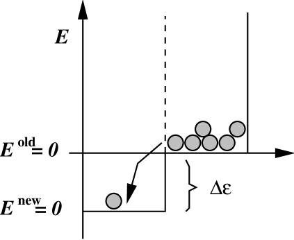
Figure 1: “Energies” (inferiorities) of strings in a first-order phase transition with latent heat $\Delta\epsilon$.

This bubble expands with a speed given by the Fisher velocity

$$v\sim\sqrt{D\Delta\epsilon}\;,$$ (4)

where $D$ is the diffusion coefficient (of information) in this medium, until the entire population has been converted (Chu and Adami 1997). This marks the end of the phase transition, as the population returns to equilibrium via mutations acting on the new species, creating new diversity and restoring the entropy of the population to its previous value. This prepares the stage for a new avalanche, as only an equilibrated population is vulnerable to even the smallest perturbation. The system has returned to a critical point, driven by mutations, self-organized by information.

Thus we see how a first-order scenario, without coevolution, can lead to self-organized and critical dynamics. It takes place within a single, finite, ecological niche, and thus does not contradict the dynamics taking place for populations that span many niches. Rather, we must conclude that the descriptions complement each other, from the single-niche level to the ecological web. Let us now take a closer look at the statistics of avalanches in this model, i.e., at the distribution of genotype sizes.

Exponents and Power Laws

The size of an avalanche in this particular system can be approximated by the size $s$ of the genotype that gave rise to it, Eq. (2). We shall measure the distribution of these sizes $P(s)$ in the Artificial Life system Avida, which implements a population of self-replicating computer programs written in a simple machine language-like instruction set of ${\cal D}=24$ instructions, with programs of varying sequence length. In the course of self-replication, these programs produce mutant off-spring because the copy instruction they use is flawed at a rate $R$ errors per instruction copied, and adapt to an environment in which the performance of logical computations on externally provided numbers is akin to the catalysis of chemical reactions (Ofria, Brown and Adami 1998). In this artificial chemistry therefore, successful computations accelerate the metabolism (i.e., the CPU) of those strings that carry the gene (code) necessary to perform the trick, and any program discovering a new trick is the seed of another avalanche.

Avida is not a stirred-reactor environment (although one can be simulated). Rather, the programs live on a two-dimensional grid, each program occupying one site. The size of the grid is finite, and chosen in these experiments to be small enough that avalanches are generally over before a new one starts. As is well-known, this is the condition sine qua non for the observation of SOC behavior, a separation of time scales which implies that the system is driven at infinitesimal rates.

Let $\tau$ denote the average duration of an avalanche. Then, a separation of time scales occurs if the average time between the production of new seeds of avalanches is much larger than $\tau$. New seeds, in turn, are produced with a frequency $\langle\epsilon\rangle P$, where $\langle\epsilon\rangle$ is again the average replication rate, and $P$ is the mutation probability (per replication period) for an average sequence of length $\ell$,

$$P=1-(1-R)^{\ell}\;.$$ (5)

For small enough $R$ and not too large $\ell$ (so that the product $R\ell$ is smaller than unity) we can approximate $P\approx R\ell$, and infinitesimal driving occurs in the limit

$$\langle\epsilon\rangle R\ell\ll\frac{1}{\tau}\;.$$ (6)

Furthermore

$$\tau\sim\frac{L}{v}$$ (7)

with $L$ the diameter of the system and $v$ a typical Fisher velocity. The fastest waves are those for which the latent heat is of the order of the new fitness, i.e., $\Delta\epsilon\sim\epsilon$, in which case $v\approx\epsilon$ (because $D\sim\epsilon$ in Eq. (4), see Chu and Adami 1995) and a separation of time scales is assured whenever

$$\frac{1}{R\ell}\gg{L}\;,$$ (8)

that is, in the limit of vanishing mutation rate or small population sizes. For the $L=60$ system used here, this condition is obeyed (for the fastest waves) only for the smallest mutation rate tested and sequence lengths of the order of the ancestor.

Figure 2: Fitness of the dominant genotype in the population, $\epsilon_{\rm best}$ as a function of time (in updates).

In the following, we keep the population size constant (a $60\times 60$ grid) and vary the mutation rate. From the previous arguments, we expect true scale-free dynamics only to appear in the limit of small mutation rates. As in this limit avalanches occur less and less frequently, this is also the limit where data are increasingly difficult to obtain, and other finite size effects can come into play. We shall try to isolate the scale-free regime by fitting the distribution to a power law

$$P(s)\sim s^{-D(R)}$$ (9)

and monitor the behavior of $D$ from low to high mutation rates.

In Fig. 2, we display a typical history of $\epsilon_{\rm best}$, i.e., the fitness of the dominant genotype. Note the “staircase” structure of the curve reflecting the “punctuated” dynamics, where each step reflects a new avalanche and concurrently an extinction event. Staircases very much like these are also observed in adapting populations of E. Coli (Lenski and Travisano 1994).

As touched upon earlier, the Avida world represents an environment replete with information, which we encode by providing bonuses for performing logical computations on externally provided (random) numbers. The computations rewarded usually involve two inputs $A$ and $B$, are finite in number and listed in Table 1. At the end of a typical run (such as Fig. 2) the population of programs is usually proficient in almost all tasks for which bonuses are given out, and the genome length has grown to several multiples of the initial size to accommodate the acquired information.

Table 1: Logical calculations on random inputs $A$ and $B$ rewarded, bonuses, and difficulty (in minimum number of nand instructions required). Bonuses $b_{i}$ increase the speed of a CPU by a factor $\nu_{i}=1+2^{b_{i}-3}$.

Name	Result	Bonus $b_{i}$	Difficulty
Echo	I/O	1	–
Not	$\neg A$	2	1
Nand	$\neg(A\wedge B)$	2	1
Not Or	$\neg A\vee B$	3	2
And	$A\wedge B$	3	2
Or	$A\vee B$	4	3
And Not	$A\wedge\neg B$	4	3
Nor	$\neg(A\vee B)$	5	4
Xor	$A\ {\rm xor}\ B$	6	4
Equals	$\neg(A\ {\rm xor}\ B)$	6	4

Because the amount of information stored in the landscape is finite, adaptation, and the associated avalanches, must stop when the population has exhausted the landscape. However, we shall see that even a ‘flat’ landscape (on which evolution is essentially neutral after the sequence has optimized its replicative strategy ) gives rise to a power law of genotype sizes, as long as the programs do not harbor an excessive amount of “junk” instructions. A typical abundance distribution (for the run depicted in Fig. 2) is shown in Fig. 3.

Figure 3: Distribution of genotypes sizes $P(s)$ fitted to a power law (solid line) at mutation rate $R=0.004$.

As mentioned earlier, we can also turn off all bonuses listed in Tab. 1, in which case fitness is related to replicative abilities only. Still, avalanches occur (within the first 50,000 updates monitored) due to minute improvements in fitness, but the length of the genomes typically stays in the range of the ancestor, a program of length 31 instructions. We expect a change of dynamics once the “true” maximum of the local fitness landscape is reached, however, we did not reach this regime in the experiments presented here. The distribution of genotype sizes for the flat landscape is depicted in Fig. 4.

Figure 4: Distribution of genotypes sizes $P(s)$ for a landscape devoid of the bonuses listed in Tab. 1, at mutation rate $R=0.003$.

Clearly then, even such landscapes (flat with respect to all other activities except replication) are not neutral. Indeed, it is known that neutral evolution, where the chance for a genotype to increase or decrease in number is even, leads to a power law in the abundance distribution with exponent $D=1.5$ (Adami, Brown, and Haggerty, 1995).

Figure 5: Fitted exponent of power law for 34 runs at mutation rates between $R=0.0005$ and $R=0.01$ copy errors per instruction copied. The error bars reflect the standard deviation across the sample of runs taken at each mutation rate. The solid line is to guide the eye only.

In order to test the dependence of the fitted exponent $D(R)$ [Eq. (9)] on the mutation rate, we conduct a set of experiments at varying copy-mutation rates from $0.5\times 10^{-3}$ to $10\times 10^{-3}$ and take data for 50,000 updates. Again, a “best” genotype is not reached after this time, and we must assume that avalanches were still occurring at the end of these runs. Furthermore, in some runs we find that a genotype comes to dominate the population (usually after most ‘genes’ have been discovered) which carries an unusual amount of junk instructions. As mentioned earlier, such species produce a distribution that is exponentially suppressed at large genotype sizes (data not shown). To avoid contamination from such species, we stop recording genotypes after a plateau of fitness was reached, i.e., if the population had discovered most of the bonuses. Furthermore, in order to minimize finite size effects on the determination of the critical exponent, we excluded from this fit all genotype abundances larger than 15, i.e., we only fitted the smallest abundances. Indeed, at larger mutation rates the higher abundances are contaminated by a pile-up effect due to the toroidal geometry, while at lower mutation rates a scale appears to enter which prevents scale-free behavior. We have not, as yet, been able to determine the origin of this scale.

In the results reported here, we show the dependence of the fitted exponent $D$ as a function of the mutation rate $R$ used in the run, which, however, is a good measure of the mutation probability $P$ only at small $R$ and if the sequence length is not excessive. As a consequence, data points at large $R$, as well as runs where an excessive sequence length developed, carry a systematic error.

For the 34 runs that we obtained, the power $D$ was measured for each run (for the low abundances), and an average was calculated for all the runs at a particular mutation rate. This data is plotted in Fig. 5 and shows a plateau in the fitted exponent only at intermediate mutation rates, with $D=2.0\pm 0.05$. A fit of the middle abundances (10-100) produces a critical coefficient more or less independent of mutation rate, around $D=2.0$, but with less accuracy (data not shown). At high $R$, we witness a deviation from scale-free behavior (reflected in the rising $D$ for small abundances) which is most likely due to pile-up, i.e., a finite toroidal lattice. This effect may be avoided by using absorbing rather than periodic boundary conditions. We also see a violation of scaling at small $R$, which is due to the emergence of some other scale. While it is most likely a finite-size effect, the exact origin of this scale is as yet unclear. We comment on the significance of these results in Section V.

Still, more control over the spread in exponents for fixed mutation rate would be desirable. This can obviously be achieved by plotting $D$ versus $P$, rather than $R$, for example, and by better keeping track of the coding percentage within a genotype, a variable that we know significantly affects the shape of the distribution. Such experiments are planned for the near future.

Distribution of Species Sizes

In Avida, it is possible to monitor groups of programs that display the same “phenotype”, while differing in genotype. Even though programs in this world are haploid (single-stranded) and do not reproduce sexually, it is convenient to label such groups taxonomically, i.e., we refer to them as “species”. Strictly speaking, a species consists out of all those genotypes that, when executed, give rise to the same “chemistry”, i.e., such programs differ only in instructions that are either unexecuted, or else are neutral. Algorithmically, the determination whether two genotypes belong to the same species is complicated by the fact that sequence length is not constant in these experiments. Thus, we need to be able to compare strings with differing lengths, which is achieved by lining them up in such a manner that they are identical in the maximum number of corresponding sites. Subsequently, a cross-over point is chosen randomly and the genomes above and below this point are swapped. In other words, we construct a hybrid program from the two candidates and test it for functionality, but without introducing it in the population (see Adami 1998.) In the experiments reported here, we actually test two cross-over points in order to rule out accidental matches. In retrospect, we find that almost all those strings classified as belonging to the same species by this method differ only in “silent”, or at least inconsequential, instructions.

The abundance distribution of genotypes within species more closely corresponds to the kind of geometric distributions investigated by Willis (1922) as well as Burlando (1990, 1993). Indeed, Burlando found, in an analysis of distributions of subtaxa within taxa obtained from the fossil record as well as recorded flora and fauna, that these distributions appear to be scale-free across taxonomic hierarchies, with critical coefficients between $2.0<D<2.5$. This distribution can also be viewed as a distribution of avalanches sizes, if avalanches are redefined as events that spawn different genotypes of the same species. Indeed, in this manner it is possible to investigate hierarchies of avalanches, each higher level presumably sporting a higher critical coefficient.

In the experiments reported here, we found species coefficients closer to $D\approx 2.5$, but we also found violations of power-law behavior which are most likely due to the contribution of species of different lengths to the abundance distribution. Indeed, the amount of “junk” instructions in a species most likely governs the steepness of the distribution, and several different such species may give rise to a multifractal distribution rather than a pure power law. In the future, we expect to disentangle such distributions by appealing to a an even higher level in taxonomy, reuniting all species of the same sequence length within a genus. The latter taxonomic level could, for example, be entirely phenotypic, by keeping track of which tasks a genus executes (irrespective of its genotype).

Still, even though changing sequence lengths affect the distribution of genotypes within species, those experiments in which the sequence length does not change significantly can give rise to power laws with single exponents, as shown below in Fig. 6. The data for this experiment were obtained from the same run as gave rise to Figs. 2 and 3.

Figure 6: Distribution of genotypes within species at $R=0.004$, fitted to a power law with $D=2.44\pm 0.05$.

Conclusions

The distribution of avalanche sizes in evolving systems, which is quite clearly related to the distribution of extinction events, can reveal a fair amount of information about the dynamics of the adapting agents. For example, purely random systems in which there are no fitness advantages, and where selection does not occur, can still show power law behavior, as extinction events are governed by the return-to-zero probability of random walks (Adami, Brown and Haggerty 1995). In Avida, we observe a scaling exponent $D=2.0$ in an intermediate regime of mutation rates. While it is still unclear whether the mixing of scales that we have observed at small and large mutation rates is due to the finite size of the lattice or the emergence of another scale, we can conclude with confidence that scale-free dynamics does occur. Scaling violations should be investigated by a thorough finite lattice-size analysis, and this is planned for the future along with more refined methods for dealing with explicit neutrality (i.e., “junk” code.)

An interesting hint at what the distribution might be like in Nature comes from Raup’s analysis of a data set prepared by Sepkoski (Raup 1991): genera of marine invertebrates from the fossil record. Raup’s “kill-curve” can be transformed into a distribution of sizes of extinction evens (as shown by Newman 1996) governed by a critical exponent close to $D=2.0$. This is tantalizingly close to the coefficient we found in our genotype abundance distribution, but we must be careful in comparing these distributions.

The avalanche-size distribution of genotypes gives us a good indication of the strength of an evolutionary shock, but also about the length of time the particular species dominates the dynamics, and therefore, of the time between evolutionary transitions. Also, each evolutionary transition brings with it a wave of extinction, as all previously extant genotypes and species of lower fitness must disappear on the heels of the new “discovery”. The size of extinction events proper, however, is not measured by the “epoch-length” distribution reflected in the avalanche sizes, but rather by the abundance of genotypes within species (or any higher taxonomic abundance distribution) because each species appearing in this distribution must eventually go extinct, and thus this distribution must equal the distribution of extinction sizes. The latter distribution (measured in Section IV), appears to have a critical exponent around $D\approx 2.5$, higher than the corresponding one from the fossil record. Furthermore, we must keep in mind the simplicity of the model treated here when comparing to actual fossil data. As mentioned in the introduction, coevolution does not play a role in the dynamics controlling the size of avalanches in this model, while we must assume that extinctions in Earth history have some co-evolutionary component. On the other hand, the abundance distribution of genotypes within species is consistent with those obtained by Burlando (1990, 1993), who argued that they represented evidence for a “fractal geometry of Nature”.

From the present analysis, it is clear that there is as yet no reason to jump to conclusions from the evidence extracted either from the fossil record, theoretical models of extinctions (Newman 1997), or else direct implementation of the dynamics of adaptive avalanches as we have done here. We do, however, see clear evidence that avalanches not reigned in by any scale can and do develop in evolving and adapting systems without co-evolutionary pressures, via first-order transitions in populations occupying single ecological niches. Not only do we find scale-free dynamics for the time between transitions (as evidenced by the genotype abundance distribution) but also for the strength of these transitions, measured by the distribution of species-sizes. It is left for future experiments to determine how such dynamics, taking place in interacting ecological niches, gives rise to power laws for co-evolutionary systems, and how the description in terms of first-order transitions is ipso facto transmutated into a second-order scenario.

This work was supported by NSF grant No. PHY-9723972.

References

- [1] Adami, C. 1995. Self-organized criticality in living systems. Phys. Lett. A 203: 23.
- [2] Adami, C. 1998. Introduction to Artificial Life. Santa Clara: TELOS Springer-Verlag.
- [3] Adami, C. and C. T. Brown. 1994. Evolutionary learning in the 2D Artificial Life system ‘Avida’. In Artificial Life IV, edited by R.A. Brooks and P. Maes. Cambridge, MA: MIT Press, p. 377.
- [4] Adami, C., C. T. Brown and M. R. Haggerty. 1995. Abundance distributions in Artificial Life and stochastic models: ‘Age and Area’ revisited.Lect. Notes in Artif. Intell. 929: 503.
- [5] Bak, P. and M. Paczuski. 1996. In Physics of Biological Systems. Heidelberg: Springer-Verlag.
- [6] Bak, P. and K. Sneppen. 1993. Punctuated equilibrium and criticality in a simple model of evolution. Phys. Rev. Lett. 71: 4083.
- [Bak, Tang, and Wiesenfeld, 1987] Bak, B., C. Tang, and K. Wiesenfeld. 1987. Self-organized criticality: An explanation of 1/ noise. Phys. Rev. Lett. 59: 381.
- [Bak, Tang, and Wiesenfeld, 1988] Bak, B., C. Tang, and K. Wiesenfeld. 1988. Self-organized criticality. Phys. Rev. A 38: 364.
- [7] Burlando, B. 1990. The fractal dimension of taxonomic systems. J. Theor. Biol. 146: 99.
- [8] Burlando, B. 1993. The fractal geometry of evolution. J. Theor. Biol. 163: 161.
- [9] Chu, J. and C. Adami. 1997. Propagation of information in populations of self-replicating code. In Proc. of Artificial Life V, edited by C. G. Langton and K. Shimohara. Cambridge, MA: MIT Press, p. 462.
- [10] Elena, S. F., V. S. Cooper and R.E. Lenski. 1996. Punctuated evolution caused by selection of rare beneficial mutations. Science 272: 1802.
- [11] Gil, L. and D. Sornette. 1996. Landau-Ginzburg theory of self-organized criticality. Phys. Rev. Lett. 76: 3991.
- [12] Gould, S. J. and N. Eldredge. 1977. Punctuated equilibria: The tempo and mode of evolution reconsidered. Paleobiology 3: 115.
- [13] Gould, S. J. and N. Eldredge. 1993. Punctuated equilibrium comes of age. Nature 366: 223.
- [14] Lenski, R. and M. Travisano. 1994. Dynamics of adaptation and diversification–A 10,000 generation experiment with bacterial populations. Proc. Nat. Acad. Sci. 91: 6808-6814.
- [15] Newman, M. E. J. 1996. Self-organized criticality, evolution, and the fossil extinction record. Proc. Roy. Soc. B 263: 1605–1610.
- [16] Newman, M. E. J. 1997. A model of mass extinction. Eprint adap-org/9702003.
- [17] Newman, M. E. J., S. M. Fraser, K. Sneppen, and W.A. Tozier. 1997. Self-organized criticality in living systems—Comment. Phys. Lett. A 228: 202.
- [18] Ofria, C., C. T. Brown and C. Adami. 1998. The Avida User’s Manual. In Adami (1998). The Avida software is publicly available at ftp.krl.caltech.edu/pub/avida.
- [19] Raup, D. M. 1991. A kill curve for phanerozoic marine species. Paleobiology 17: 37–48..
- [20] Sornette, D., A. Johansen, and I. Dornic. 1995. Mapping self-organized criticality to criticality. J. de Phys. I 5: 325.
- [21] Solé, R. V. and J. Bascompte. 1996. Are critical phenomena relevant to large-scale evolution? Proc. Roy. Soc. B 263: 161–168.
- [22] Willis, J. C. 1922. Age and Area. Cambridge: Cambridge University Press.