Effects of neutral selection on
the evolution of molecular species

Abstract

We introduce a new model of evolution on a fitness landscape possessing a tunable degree of neutrality. The model allows us to study the general properties of molecular species undergoing neutral evolution. We find that a number of phenomena seen in RNA sequence-structure maps are present also in our general model. Examples are the occurrence of “common” structures which occupy a fraction of the genotype space which tends to unity as the length of the genotype increases, and the formation of percolating neutral networks which cover the genotype space in such a way that a member of such a network can be found within a small radius of any point in the space. We also describe a number of new phenomena which appear to be general properties of neutrally evolving systems. In particular, we show that the maximum fitness attained during the adaptive walk of a population evolving on such a fitness landscape increases with increasing degree of neutrality, and is directly related to the fitness of the most fit percolating network.

1 Introduction

Biological molecules such as proteins and RNAs undergo evolution just as organisms do, selected for their ability to perform certain functions by the reproductive success which that ability imparts on their hosts. It is believed that many mutations of a molecule are evolutionarily neutral in the sense that they do not change the fitness of the molecule to perform the function for which it has been selected. We have many examples of proteins which appear to possess approximately the same conformation and to perform the same function in different species, but which have different sequences. Such proteins may differ only by a single amino acid or may have whole regions which have been substituted or inserted, or they may even be so different as to appear completely unrelated. A mutation is said to be neutral if it changes a molecule into one of these functional equivalents, leaving the viability of its host unchanged. This idea was first explored in detail by Kimura [1, 2].

In fact, as Ohta has pointed out [3], it is not necessary that the fitness of a molecule remain precisely the same under a given mutation for that mutation to be considered neutral. A mutation which produces a change in fitness will cause the population sizes of the original and mutant strains to diverge exponentially from one another over time. However, the time constant of this exponential is inversely proportional to the change in fitness. Thus if the change in fitness is small, its effects will be felt only on very long time-scales. If these time-scales are significantly longer than the time-scale on which mutations occur (the inverse of the mutation rate), then the change in fitness will never be felt. In effect, the mutation rate places a limit on the resolution with which selection can detect changes of fitness, so that small fitness changes are effectively, if not precisely, neutral.

It is possible that the concept of neutral selection can also be applied to the evolution of entire organisms. Certainly there are changes possible in an organism’s genome which have no immediate effect on its reproductive success, or which produce an effect sufficiently small that selection cannot detect it on the available time-scales. In this paper we will primarily use the language of molecular evolution, but the reader should bear in mind that the ideas described may have wider applicability.

Despite the long history of the idea, many aspects of neutral evolution are still not well understood. In particular, we have very little idea of the general behaviours that can be expected of systems (molecules or organisms) with a significant degree of evolutionary neutrality. The primary reason for this gap in our understanding is that, despite many decades of hard work, we still have a rather poor idea of the way in which genomic sequences map onto molecular structures and hence onto a fitness measure. In the case of entire organisms the equivalent problem is that of calculating the genotype-phenotype mapping, which is even less well understood. One simple case in which neutral evolution has been investigated in some detail is that of RNA structure [4, 5, 6, 7], although calculations so far are limited to secondary structures, and even these cannot be calculated with any reliability, so that these studies should be taken more as a qualitative guide to the behaviour of systems undergoing neutral selection than an accurate representation of the real world. The trouble with this approach however is that RNAs are not a sufficiently general model that the results gained from their study can be applied to other systems, such as protein evolution or the evolution of whole organisms.

At the other extreme, studies have been performed of extremely simple mathematical models of neutral evolution in the context of genetic algorithms [8, 9]. An example is the “Royal Road” genetic algorithm studied by van Nimwegen et al. [10, 11]. These models possess highly artificial fitness functions chosen specifically to show a high degree of neutrality whilst at the same time being simple enough to yield to analytic methods. Like RNA secondary structures, these models have given us some insight into the type of effects we may expect neutral evolution to produce, but, like RNAs, they are not sufficiently general to be sure that these insights apply to other systems as well.

In this paper, therefore, we propose a new mathematical model of neutral evolution. This model is an abstract model of a genotype to fitness map in the spirit of the Royal Road model. This approach allows us to sidestep the problems of incorporating the chemistry of real molecules in our calculations and to investigate the properties of the system more quickly and in greater detail than is possible with, for example, RNA structure calculations. In addition, the model is more general than either the Royal Road fitness function or the RNA sequence-structure maps of Refs. [5, 6]. In fact, it possesses regimes in which it mimics the behaviour of both of these systems, as well as protein- and organism-like regimes. Because the behaviours of our model cover such a wide range of possibilities, it seems reasonable to conjecture that generic features of the model which span all of these regimes may be common to most systems undergoing neutral selection. This is the power of our model, and these general results are the results that we will concentrate on in this paper; we believe that the generic behaviours of our model should be visible in the evolution of real systems such as proteins which are, as yet, beyond our abilities to study directly.

In Section 2 we introduce our landscape model of neutral evolution. In Section 3 we discuss its properties and compare these with previous results for other systems undergoing neutral evolution. In Section 4 we discuss the implications of our results for evolving molecular species. In Section 5 we give our conclusions.

2 The model

Selective neutrality arises as a result of the many-to-one nature of the sequence-structure or genotype-phenotype maps found in biological systems. Many protein sequences, for example, map onto the same tertiary structure, and since the fitness is primarily a function of the structure, such sequences possess (at least approximately) the same fitness. We wish to construct a model of this phenomenon without resorting to actual calculations of the structure of any particular class of molecules. Only in this way can we hope to create a model which is general enough to represent the behaviours of many different such classes. Our approach is to employ a “fitness landscape” model of the type first proposed by Wright [12, 13] which maps sequence (or genotype) directly to fitness. Structures (or phenotypes) appear in our model as contiguous sets or “neutral networks” of sequences possessing the same fitness.

Our model is a generalization of the $NK$ model proposed by Kauffman [14, 15], which is itself a generalization of the spin glass models of statistical physics [16]. Consider a sequence of $N$ loci, which correspond to the nucleotides in an RNA or to amino acids in the case of a protein. At each locus $i$ we have a value $x_{i}$ drawn from an appropriate alphabet, such as $\{\mbox{A,C,G,U}\}$ for RNAs, or the set of 20 amino acids in the case of proteins. We denote the size of the alphabet by $A$. Each locus interacts with a number $K$ of other “neighbour” loci, which may be chosen at random or in any other way we wish. (Kauffman refers to these interactions as epistatic interactions, though this nomenclature is strictly only appropriate to the case where we are modelling the fitness of whole organisms.) In the case of RNAs, bases most often interact with one other base to form either a Watson-Crick or a G-U pair. Some bases have both pairing and tertiary interactions. Some, in the single stranded regions, have very little interaction with any others. Thus a value of $K=1$ might be approximately correct for RNA. For proteins, which have more complex types of interactions, a higher value of $K$ may be appropriate.

Each locus $i$ makes a contribution $w_{i}$ to the fitness of the sequence, whose magnitude depends on the value $x_{i}$ at that locus and also on the values at each of the $K$ neighbouring loci. There are $A^{K+1}$ possible sets of values for the $K+1$ loci in this neighbourhood, and hence $A^{K+1}$ possible values of $w_{i}$. Following Kauffman and Johnsen [14] we choose this set of values at random. However, Kauffman and Johnsen chose the values to be random real numbers in the interval $0\leq w_{i}<1$. We by contrast choose them to be integers in the range $0\leq w_{i}<F$. Thus if $F=2$ for example, each contribution $w_{i}$ is either zero or one. Now we define the fitness $W$ of the entire sequence to be proportional to the sum of the contributions at each locus:

$$W={1\over N(F-1)}\sum_{i}w_{i}.$$ (1)

The fitness of all sequences thus falls in the range from zero to one, and there are $NF-N+1$ possible fitness values in this range.

In the limit in which $F\to\infty$ the probability that two sequences will possess the same fitness becomes vanishingly small, and our model therefore possesses no neutrality and is in fact exactly equivalent to the $NK$ model. However, when $F$ is finite the probability of two sequences possessing the same fitness is finite, so that the model possesses neutrality to a degree which increases as $F$ decreases. Neutrality is greatest when $F$ takes the smallest possible value of two. Two sequences with the same fitness may be equivalent either to molecules which fold into the same conformation and perform the same function, or they may be equivalent to molecules with different conformations but approximately the same contribution to the reproductive success of the host organism. The ruggedness of the landscape is controlled by the parameter $K$, and is largest when $K$ takes the maximal value of $N-1$ [14, 17]. In the next section, we investigate the properties of the landscapes generated by our model, and show that with the right choice of parameters they can be used to mimic real biological systems, such as RNAs.

3 Evolution on neutral landscapes

The topology of a fitness landscape depends on the types of mutation allowed to molecules evolving on it. In biological evolution, point mutations—mutations of the value at a single locus—are the most common. In this case, a neutral network is defined to be a set of sequences which all possess the same fitness and which are connected together via such point mutations. In the molecular case, we assume that closely similar sequences have the same fitness because they fold into the same conformation, so that these neutral networks correspond to (tertiary) structures. In the organismal case they correspond to phenotypes.

The model described in the last section possesses neutral networks of exactly this type. The total fitness $W$ in the model ranges from zero to one, but the greatest number of sequences have fitness close to $W=0.5$. (In the extreme case where $K=N-1$ the distribution of $W$ is binomial. When $K<N-1$ it is approximately but not exactly so. Examples of these distributions are shown in Figure 1 (a).) We would therefore expect the largest neutral networks to be those with fitness close to $W=0.5$ and this is indeed what we find in practice.

Typically there are a large number of small neutral networks and a small number of large ones. In Figure 1 we show histograms of the sizes of the neutral networks for $N=20$ and various values of $K$. For the RNA-like case $K=1$, the histogram appears to be convex, indicating a distribution which falls off faster than a power law. The same behaviour has been in seen in RNA studies by Grüner et al. [6]. As $K$ increases the distribution flattens, and by the time we reach $K=5$ it is markedly concave. Thus the behaviour seen in RNAs is not in this case generic. For some intermediate value of $K$ close to $K=2$, the distribution appears to be power-law in form, perhaps indicating the divergence of some scale parameter governing the distribution, in a manner familiar from the study of critical phenomena [18].

We find that the total number of neutral networks $S_{N}$ grows exponentially as $a^{N}$ with sequence length. In Figure 1 (b) we show the number of networks in our model for $K=1$, both for two-letter $\{\mbox{G,C}\}$ alphabets, and for a four-letter $\{\mbox{A,C,G,U}\}$ alphabet. We find that $a\approx 1.5$ for the $A=2$ case and $a\approx 2.3$ for the $A=4$ case. Interestingly, Stadler and co-workers [6, 7, 20] have performed the same calculations for RNA sequences using the full secondary-structure calculation, and they also find an exponential increase in the number of structures with sequence length with values of $a=1.6$ and $a=2.35$ for the two- and four-letter cases respectively. This suggests to us that this behaviour is more general than the specific secondary-structure map employed in the Stadler calculations.

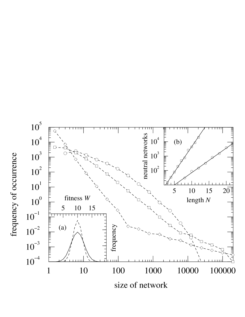
Figure 1: Histogram of the frequency of occurrence of neutral networks as a function of size for a particular realization of a landscape with $N=20$, $A=2$, $F=2$, and (circles) $K=1$, (squares) $K=2$, (diamonds) $K=5$. Inset (a): the frequency of occurrence of sequences as a function of fitness for $N=20$, $A=2$, $F=2$, and (solid line) $K=19$, (dotted line) $K=0$. Inset (b): the number of neutral networks as a function of $N$ for $K=1$, $F=2$, and (circles) $A=2$, (squares) $A=4$.

The largest neutral networks on our landscapes percolate, which is to say, they fill the sequence space roughly uniformly, in such a way that no sequence is more than a certain distance away from a member of the percolating network. Determining which networks are percolating is not an easy task. We have developed two different measures to help identify percolating networks, and we describe them further in Ref. [19]. Grüner et al. [6] introduced instead the idea of a “common” network, which is one which contains greater than the average number of sequences. We can employ this definition with our model too. We find that the common networks in the model form a small fraction of the total number of networks, that fraction decreasing exponentially as $N$ increases, as shown in the inset to Figure 2. The same result is found in RNAs [6].

In the main frame of Figure 2 we show the fraction of sequences which fall in the common networks as a function of $N$. As the figure shows, our numerical studies indicate that this fraction increases with sequence length, tending to one in the limit of large $N$. Even though the common networks form a smaller and smaller fraction of all networks as $N$ becomes large, they nonetheless cover more and more of the sequence space. These results have interesting evolutionary implications: they imply that as sequences become longer, a larger and larger majority of structures (the small networks) are vanishingly unlikely to occur through natural selection. Evolution can only find the smaller and smaller fraction of “common” structures. The same conclusions have been reached in the case of RNAs. However, the results presented here indicate that these conclusions are not specific to RNAs, and probably apply to most systems undergoing neutral evolution.

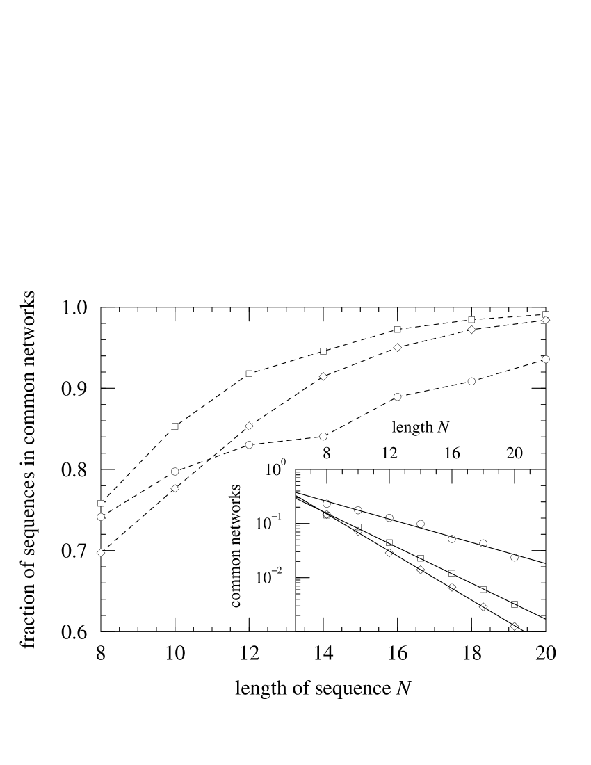
Figure 2: The fraction of all sequences which fall in common networks as a function of $N$ for a particular realization of the model with $A=2$, $F=2$, and (circles) $K=2$, (squares) $K=4$, (diamonds) $K=6$. Inset: the number of common networks as a fraction of the total number of networks for the same landscapes.

Next we have examined the dynamics of populations evolving on our landscapes. These studies have yielded some of the most interesting results of this work. In their studies with $NK$ landscapes, Kauffman and Johnsen [14] made a useful approximation in representing evolving populations by their single dominant sequence. This approximation is only valid in the case in which the time-scale for mutation is much longer than the time-scale on which selection acts. For the moment we will assume this to be the case. A “random hill-climber” is a population of this type, represented by a single dominant strain, which tries mutations—point mutations in the present case—until it finds one with higher fitness than the current strain. In this way the hill-climber performs an adaptive walk through sequences of ever-increasing fitness until it reaches a local fitness optimum. To study neutral landscapes we modify this strategy so that the hill-climber samples adjacent sequences at random until it finds one of fitness greater than or the same as itself. Such a climber will move at random on a neutral network until it finds a mutation which takes it to a network of higher fitness. In the upper curve of Figure 3 we show the average fitness attained by such a walker over ten simulations on our landscapes as a function of the neutrality parameter $F$. Recall that neutrality increases with decreasing $F$. As the figure shows, the hill-climber on average finds higher fitness maxima for higher degrees of neutrality. In other words, neutrality helps the population to attain a greater fitness. This is certainly an idea which has been entertained before in the literature, but it is lent a new conviction when we see it emerge in the behaviour of a general model such as this.

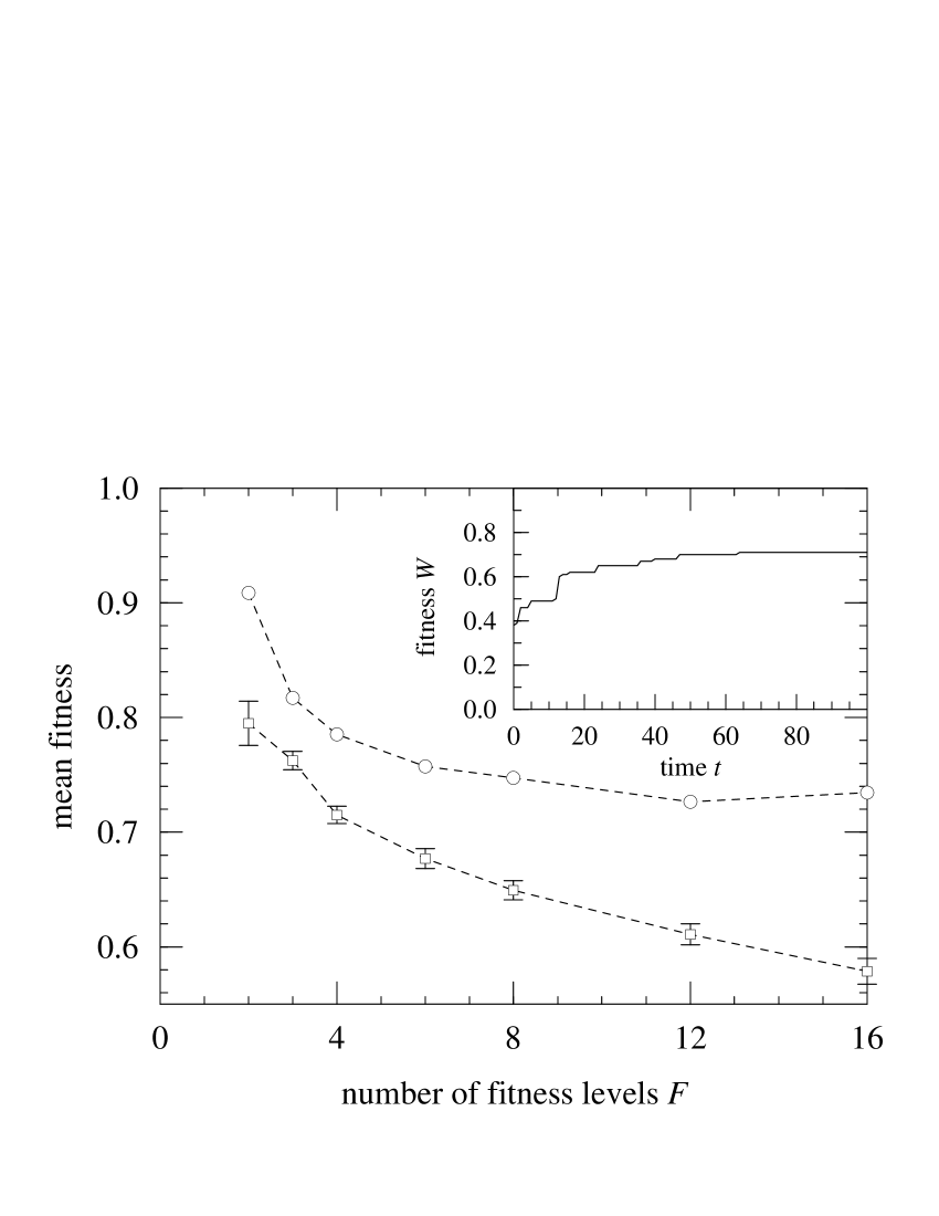
Figure 3: The maximum fitness attained by a random hill-climber averaged over ten simulations with $N=20$, $K=4$ and $A=2$, as a function of the neutrality parameter $F$ (circles). The lower curve (squares) is the fitness of the most fit percolating neutral network averaged over the same ten runs. Inset: the fitness of one of the hill-climbers in the simulation as a function of time.

The lower curve on Figure 3 shows the fitness of the most fit percolating network averaged over the same ten landscapes. The curve follows quite closely the form of the curve for the fitness of the local maxima found by the hill-climber. Our explanation of this result is as follows. The climber moves diffusively on a neutral network until it finds a one-mutant neighbour which belongs to a network of greater fitness, at which point it shifts to that network. This process continues until it reaches a non-percolating network, at which point it is confined to the region occupied by the network and can only get as high as the local maximum within that region. Thus the highest fitness attainable on a landscape with neutrality depends directly on the highest fitness at which there are percolating networks. Since the landscapes with the greatest degree of neutrality also have more and fitter percolating networks, this explains why higher fitnesses are attained on landscapes with lower values of $F$.

The inset to Figure 3 shows the fitness of one of our hill-climbers as a function of time, and we can clearly see the steps in this function where the climber finds its way onto a neutral network of higher fitness. Similar steps have been seen, for example, in laboratory experiments on the evolution of bacteria [21, 22]. Although it appears in the figure that nothing happens in the periods between these jumps, it is at these times that the climber diffuses around its network, testing new mutations to find one of higher fitness. It is this diffusive motion which allows us to find higher fitness sequences on landscapes with higher degrees of neutrality. Van Nimwegen et al. [10] have dubbed these periods of apparent stasis “epochs”. They also bear some similarity to the palaeontological “punctuated equilibria” described by Eldredge and Gould [23, 24], although there are many other possible explanations for the periods of stasis seen in fossil evolution.

To investigate the epochs in more detail, we have performed simulations of true populations evolving on our landscape. In these simulations we take a population of $M$ sequences which at each generation reproduce with probability proportional to their fitness, in such a way that the total population size remains constant. Reproduction is also subject to mutation at some rate $q$ per locus: with probability $q$ the value at any locus in a sequence changes to a new randomly chosen one when the sequence is reproduced.

Figure 4: Solid line: the average fitness of a population of $M=1000$ sequences evolving on a landscape with $N=20$, $K=4$, $A=2$ and $F=2$. The mutation rate is $q=5\times 10^{-6}$. Dotted line: the entropy of the population, which is a measure of the diversity of sequences present.

In Figure 4 we show the results of such a simulation for a population of $M=1000$ sequences with $N=20$ and a mutation rate of $q=5\times 10^{-6}$. For this value of $q$ the mutation rate is low enough that the hill-climber approximation used above is reasonable and, as the figure shows, the epochs visible in the case of the hill-climber appear also in the average fitness measured in the population simulations (solid line). For the simple case of the Royal Road genetic algorithm, van Nimwegen et al. [11] have studied the epochs extensively and given a number of analytic and numerical results which may generalize to present case.

The length of the epochs in Figures 3 and 4 increase, on average, with increasing fitness. This behaviour was also seen in the Royal Road, and occurs because as the fitness increases the number of structures with higher fitness still dwindles. The length of the epochs in fact depends on the rate of diffusion of the population across the neutral network, which in turn depends on $q$, and on the density of “points of contact” between the network and other networks of higher fitness [2]. Another interesting feature of the epochs, also seen in the Royal Road, is that their average fitness does not correspond exactly to the fitness of any of the networks. Typically the average fitness is a little lower than the fitness of the dominant structure in the population because deleterious mutants are constantly arising. Even though these mutants are selected against, there are at any time enough of them in the population to make a noticeable difference to the average fitness. Since the number of possible mutants with lower fitness than the dominant sequence increases with increasing fitness, it is also possible to get error threshold effects with increasing fitness [25, 26]. As the fitness increases, there may come a point where the rate at which deleterious mutants arise in the population exceeds the rate at which they are suppressed by selection, and at this point further improvement in fitness becomes impossible. Thus there may be a dynamical limit on the fitness of populations, independent of the limit imposed by the structure of the landscape discussed above. (This is true of landscapes without neutral evolution too, though the effect is much more prominent in the neutral case.)

In Figure 4 we also show the entropy of the population as a function of time (dotted line). The entropy is defined as

$$S=-\sum_{i}p_{i}\log p_{i},$$ (2)

where $p_{i}$ is the average probability of finding a particular member of the population with sequence $i$. In this case, we see that the entropy is low during the epochs, indicating that the population is compact, and hence that the strong-selection approximation made in the case of the random hill-climber applies. Only during the selection events themselves, when the population moves to a new neutral network does the entropy increase.

Simulations similar in spirit to ours have been performed for populations of tRNAs by Fontana and co-workers [5, 27]. In these simulations the authors chose a “target” structure which was artificially selected for, and they also observed epochs in the evolution as the population passed through a succession of increasingly fit structures on its way to the target.

4 Discussion

The aim of this work is to study a model of neutral evolution which is general enough to encompass behaviours typical of other more specific models which have been employed in the past. In this way we can reproduce in a general context the results which have been observed as special cases and hence investigate the extent to which these results are general properties of fitness landscapes possessing neutrality, or particular to the systems in which they were first observed. In this spirit, we put forward the following conjectures about the fitness landscapes on which biological molecules evolve, based on the results of the investigations outlined in this paper.

1. The total number of possible structures increases exponentially with sequence length. The exponential constant of this increase appears to be approximately numerically equal in both the general model and the only specific case in which it has been studied, that of RNA secondary structure.

2. There are a large number of structures which correspond to a small number of sequences, and a small number of structures which correspond to a large number of sequences. The exact form of the histogram of structure frequency, shown in Figure 1, varies depending on the parameters of our model. However, for certain values of the parameters it has a form similar to that seen in RNA studies, whilst for others it appears to follow a power law.

3. The “common” structures—ones which correspond to a large number of sequences—constitute an exponentially decreasing fraction of the total number as sequence length increases. Conversely, however, they cover a fraction of the sequence space which tends to unity for long sequences.

4. The evolution of populations, at least on short time-scales, is dominated by the presence of neutrality. Neutrality helps the population to find structures of high fitness without having to cross fitness barriers. The highest fitness which can be found in this way is closely related to the fitness of the highest percolating neutral network, which itself depends on the amount of neutrality. For landscapes with a higher degree of neutrality therefore, the population typically reaches a higher fitness.

5. The fitness may be limited by error threshold effects, which are particularly severe for landscapes of this type, because the size of the neutral networks (and hence the ratio of numbers of beneficial and harmful mutants) falls exponentially with increasing fitness.

6. Evolution proceeds in jumps separated by “epochs” in which the fitness appears to change very little. In fact, the population uses these epochs to diffuse across the current neutral network, allowing it to search a larger portion of sequence space for beneficial mutations.

5 Conclusions

To conclude, we believe that by studying a simple and general model of a neutral landscape, we should be able to distinguish properties of specific systems undergoing neutral selection from properties common to all such systems. We have found a number of potential candidates for inclusion in a list of such common properties. There are many interesting lines of investigation which we have not been able to pursue in this short work, including details of the structure and size of the neutral networks such as percolation measures and covering radii, details of population dynamics on these networks including entropy and other statistical measures of the structure of such populations, calculations of the length of epochs, of the maximum fitness obtainable on these landscapes, of the effects of error threshold effects on maximum fitness, and many effects of the variation of the parameters of the model, particularly the effects of the variation of the level of epistasis $K$ and the neutrality parameter $F$. Some of these questions will be addressed in a forthcoming work.

References

- [1] Kimura, M. 1955 Solution of a process of random genetic drift with a continuous model. Proc. Natl. Acad. Sci. USA 41, 144.
- [2] Kimura, M. 1983 The Neutral Theory of Molecular Evolution. Cambridge University Press.
- [3] Ohta, T. 1972 Population size and rate of evolution. J. Mol. Evol. 1, 305.
- [4] Schuster, P., Fontana, W., Stadler, P. F. and Hofacker, I. L. 1994 From sequences to shapes and back: A case study in RNA secondary structures. Proc. R. Soc. London B 255, 279.
- [5] Huynen, M., Stadler, P. F. and Fontana, W. 1996 Smoothness within ruggedness: The role of neutrality in adaptation. Proc. Nat. Acad. Sci. USA 93, 397.
- [6] Grüner, W., Giegerich, R., Strothmann, D., Reidys, C., Weber, J., Hofacker, I. L., Stadler, P. F. and Schuster, P. 1996 Analysis of RNA sequence structure maps by exhaustive enumeration: neutral networks. Mh. Chem. 127, 355.
- [7] Grüner, W., Giegerich, R., Strothmann, D., Reidys, C., Weber, J., Hofacker, I. L., Stadler, P. F. and Schuster, P. 1996 Analysis of RNA sequence structure maps by exhaustive enumeration: structure of neutral networks and shape space covering. Mh. Chem. 127, 375.
- [8] Mitchell, M. 1996 An Introduction to Genetic Algorithms, MIT Press, Cambridge, Mass.
- [9] Prügel-Bennett, A. and Shapiro, J. 1994 An analysis of genetic algorithms using statistical mechanics. Phys. Rev. Lett. 72, 1305.
- [10] van Nimwegen, E., Crutchfield, J. P. and Mitchell, M. 1997 Finite populations induce metastability in evolutionary search. Phys. Lett. A 229, 144.
- [11] van Nimwegen, E., Crutchfield, J. P. and Mitchell, M. 1997 Statistical Dynamics of the Royal Road Genetic Algorithm. Theor. Comp. Sci., in press.
- [12] Wright, S. 1967 Surfaces of selective value. Proc. Nat. Acad. Sci. 58, 165.
- [13] Wright, S. 1982 Character change, speciation and the higher taxa. Evolution 36, 427.
- [14] Kauffman, S. A. and Johnsen, S. 1991 Coevolution to the edge of chaos: Coupled fitness landscapes, poised states, and coevolutionary avalanches. J. Theor. Biol. 149, 467.
- [15] Kauffman, S. A. 1992 The Origins of Order, Oxford University Press, Oxford.
- [16] Fischer, K. H. and Hertz, J. A. 1991 Spin Glasses, Cambridge University Press, Cambridge.
- [17] Weinberger, E. D. 1991 Local properties of the model, a tunably rugged energy landscape. Phys. Rev. A 44, 6399.
- [18] Binney, J. J., Dowrick, N. J., Fisher, A. J. and Newman, M. E. J. 1992 The Theory of Critical Phenomena, Oxford University Press, Oxford.
- [19] Newman, M. E. J. and Engelhardt, R. 1998 A model of neutral molecular evolution. In preparation.
- [20] Stadler, P. F. and Haslinger C., 1997 RNA structures with pseudoknots. Submitted to Bull. Math. Biol.
- [21] R. E. Lenski and M. Travisano, Dynamics of adaptation and diversification: a 10,000-generation experiment with bacterial populations. Proc. Natl. Acad. Sci. 91, 6080 (1994).
- [22] P. D. Sniegowski, P. J. Gerrish, and R. E. Lenski, Evolution of high mutation-rates in experimental populations of Escherichia Coli. Nature 387, 703 (1997).
- [23] Eldredge, N. and Gould, S. J. 1972 Punctuated equilibria: an alternative to phyletic gradualism. In Models in Paleobiology, T. J. M. Schopf (Ed.), Freeman, San Francisco.
- [24] Gould, S. J. and Eldredge, N. 1993 Punctuated equilibrium comes of age. Nature 366, 223.
- [25] Eigen, M. and Schuster, P. 1979 The Hypercycle: A principle of natural self-organization, Spinger, New York.
- [26] Swetina, J. and Schuster. P. 1982 Self-replication with error: A model for polynucleotide replication. Biophys. Chem. 16, 329.
- [27] Fontana, W. and Schuster, P. 1987 A computer model of evolutionary optimization. Biophys. Chem. 26, 123.