Early-time critical dynamics of lattices of coupled chaotic maps

Abstract

The early-time critical dynamics of continuous, Ising-like phase transitions is studied numerically for two-dimensional lattices of coupled chaotic maps. Emphasis is laid on obtaining accurate estimates of the dynamic critical exponents $\theta^{\prime}$ and $z$. The critical points of five different models are investigated, varying the mode of update, the coupling, and the local map. Our results suggest that the nature of update is a relevant parameter for dynamic universality classes of extended dynamical systems, generalizing results obtained previously for the static properties. They also indicate that the universality observed for the static properties of Ising-like transitions of synchronously-updated systems does not hold for their dynamic critical properties.

I Introduction

The last decade has seen considerable experimental, numerical, and analytical effort aimed at better understanding the sustained spatio-temporally chaotic regimes of large, homogeneous systems kept far-from-equilibrium by an external driving force. In particular, detailed investigation of a number of hydrodynamical flow regimes, including convection, shear flow, and crispation experiments, has led to a wealth of interesting insights into the properties of spatio-temporal chaos [1]. Important pending questions concern the status of the asymptotic limit of long time and large system size, as well as the relationship which may exist between classical equilibrium statistical mechanics and possible statistical descriptions of spatio-temporal chaos in this “thermodynamic” limit [1, 2].

This article focuses on the critical behavior of models of spatio-temporal chaos close to second-order-like phase transitions which occur in the thermodynamic limit. Theoretical work [3] has suggested that phase transitions in generic non-equilibrium systems made up of locally interacting subunits belong to the universality class of Model A [4], for both static and dynamic critical exponents, provided that the order parameter is a non-conserved, scalar quantity. Being based on coarse-grained Langevin descriptions, the approach developed in [3] overlooks the exact nature of microscopic time-evolution. Its conclusion also relies on the validity of assumptions generally associated with the dynamic renormalization group formalism.

Another significant contribution is that of Miller and Huse. In [5], they introduce a simple lattice dynamical system with microscopic Ising symmetry (square lattice of locally-coupled, chaotic, odd maps), whose salient feature is the presence of a non-equilibrium continuous transition qualitatively similar to the ferromagnetic critical point of the two-dimensional Ising model. Ising-like transitions between spatio-temporally chaotic phases turn out to be a fairly common feature of coupled maps lattices (CMLs): they are observed for a variety of local maps, lattice geometries, and update rules [6, 7, 8, 9]. However, contrary to the conjecture of [3] and to early conclusions based on simulations of much smaller systems [5], careful analysis of finite-size data obtained from extensive numerical simulations of the Miller-Huse model shows that the corresponding phase transition does not belong to the Ising universality class [7, 8]. The measured correlation-length exponent $\nu=0.89\pm 0.02$ is significantly lower than $\nu_{\rm Ising}=1$, while exponent ratios $\beta/\nu$ and $\gamma/\nu$ remain in good agreement with Ising values. Comparison with related models, in particular with transitions of sequentially-updated lattice dynamical systems, further indicates that synchronous update is the relevant parameter responsible for departure from Ising universality: keeping all other features of the Miller-Huse model unchanged, Ising static exponents are recovered as soon as sites are updated sequentially [8].

Our main objective is to extend previous work on static critical exponents to the dynamic critical properties of the Miller-Huse model. The dynamic critical exponent $z$, which quantifies the algebraic divergence of coherence times at criticality, is known to be sensitive to parameters otherwise irrelevant for static exponents, such as the existence or absence of macroscopic quantities conserved under time-evolution [4]. In addition, the nature of update is a relevant parameter for dynamical universality classes of Ising systems: synchronous update of clusters of spins yields distinct, significantly lower values of the dynamic exponent $z$ than is observed for standard sequential or checkerboard update [10]. Ignoring both the conjecture of [3] and the numerical results of [8], one may thus naively expect phase transitions of synchronously and sequentially updated CMLs to be characterized by different dynamical exponents. Here, we want to confirm, for the dynamic properties of Ising-like transitions of lattices of coupled chaotic maps, the relevance of the mode of update already discovered in [8] for their static properties. Similarly, the static universality class observed for synchronously-updated models is revisited from the point of view of their dynamical properties.

Compared to Ising systems, the measurement of static critical exponents turns out to be significantly more resource-consuming in the case of CMLs, due in particular to the presence of unusually large corrections to scaling [8]. Moreover, extracting reliable values of dynamic critical exponents from direct simulations is a notably difficult task, even in a priori simpler cases. Despite much numerical effort, the value of the dynamical exponent $z$ of Model A in dimension $d=2$ remains somewhat controversial (see [11] for a survey of work done prior to 1993, and [12] for a more recent review). The methodology we apply here to phase transitions of CMLs is based on recent theoretical work by Janssen et al., which proves the existence of a new universal regime in the early critical dynamics of systems starting from non-equilibrium (e.g. completely disordered) initial conditions [13, 14]. This regime, termed “initial critical slip” or “universal short-time behavior” in the literature, is characterized by a new non-trivial exponent $\theta^{\prime}$, unrelated to the usual static and dynamical exponents. The dynamical exponents $\theta^{\prime}$ and $z$ can be readily obtained from the initial scaling properties of observables of finite-size systems, as shown analytically in [15], and first implemented numerically in [16]. Unlike standard methods, this procedure is nearly free from the difficulties associated with critical slowing down at the transition point: useful simulation times ($T\sim 10^{2}-10^{3}$) are typically much shorter than the finite-size coherence time-scale $t_{L}\sim L^{z}$. Statistical accuracy is ensured by ensemble-averaging over a large number of independent realizations. Thanks to high numerical efficiency, good agreement on the value of critical quantities such as $\theta^{\prime}$ and $d/z-\theta^{\prime}$ has been already reached for Model A [17, 18, 19]. This makes comparison with other systems easier, and opens the way to an investigation of the relative universality of $z$ and $\theta^{\prime}$ which, based on the theoretical work of Janssen et al [13, 14], are expected to depend on the same relevant parameters.

This article is organized as follows: current understanding of early-time critical dynamics is briefly reviewed in Sec. II. The methodology we follow closely parallels that used by Okano et al. for of the two-dimensional Ising model with heat-bath and Metropolis algorithm [19]. The same procedure is used throughout, thus allowing meaningful comparison between exponents obtained for different CMLs, as well as with exponents of Model A. First, the dynamic critical properties of the Miller-Huse model, a lattice dynamical system with synchronous update, are investigated in Sec. III. The model and its phenomenology are introduced in Sec III A. Simulations pertaining to the measure of the critical exponents $\theta^{\prime}$ and $z$ are next described in Sec. III B and III C respectively. In Sec. IV, we investigate the role played by the type of update for the dynamic critical properties of Ising-like transitions, in order to extend its relevance, already established in [8] at the static level. In Sec. IV A, we first consider a sequentially updated model introduced in [8], which, according to previous numerical results, belongs to the Ising universality class for static critical exponents. In Sec. IV B, we turn to Sakaguchi’s model [9], a CML with checkerboard update whose static critical exponents are known exactly to be equal to those of the Ising model. Next, we consider, in Sec.V, various synchronously-updated models to investigate whether the universality of the static critical properties of their Ising-like transitions extend to their dynamic exponents. Our results are summed up and discussed in Sec. VI.

II Early-time critical dynamics at second-order transitions

In order to measure the dynamic critical exponent $z$ from numerical simulations of finite-size systems, most methods considered until a few years ago made use of the so-called nonlinear relaxation regime, by, e.g., looking at the decay of the system’s time-dependent magnetization $M(t)$ according to:

$$M(t)\sim t^{-\beta/(\nu z)},$$ (1)

or similar relations involving higher-order moments. This regime was generally believed to be relevant within the time interval $1\ll t\ll t_{L}$, whereas finite-size linear relaxation eventually prevails beyond $t_{L}=L^{z}$, where the magnetization decays exponentially: $M(t)\sim\exp(-t/t_{L})$.

A point overlooked until the work of Janssen et al. [13] is the importance of initial conditions. Suppose that we start from disordered non-equilibrium initial conditions (magnetization is zero or very close to zero) with very short initial correlation length, and quench the system to its critical point. One qualitatively expects fluctuations to be negligible at first: the system is then mean-field-like. Since the mean-field critical temperature is usually larger than the actual critical temperature, the system is in its ordered phase, and the magnetization (and correlation length) will want to grow. This accounts for initial magnetization growth. There is of course a crossover point, after which the system’s behavior reverts to the usual (relaxational) behavior of Eq. 1.

This qualitative idea has been formalized, and the influence of initial conditions on renormalization-group transformations investigated in detail for bulk systems [13, 14]. Let $m_{0}$ be the initial magnetization at time $t=0$. This field gives way to a new scaling index $x_{0}$ independent from already known ones (both static and dynamical), and to a timescale $t_{0}$ within which a new universal scaling regime sets in. The new exponent $\theta^{\prime}$ is universal in the same sense as the ususal dynamic critical exponent $z$, since it was obtained within the same formalism. For $t_{\rm mic}\leq t\leq t_{0}$, and $m_{0}$ small enough, the magnetization grows as a power law:

$$M(t)\sim m_{0}t^{\theta^{\prime}},$$ (2)

where $\theta^{\prime}=(x_{0}-\beta/\nu)/z$. The microscopic time $t_{\rm mic}$ is the time after which macroscopically correlated regions form, i.e. regions large compared to the microscopic length scale, in this case the lattice constant. The time-evolution of observables for $t\leq t_{\rm mic}$ is nonuniversal, and depends on microscopic features of the model. The crossover time $t_{0}$ is obtained by matching Eqns. (1) and (2):

$$t_{0}\sim m_{0}^{-x_{0}/z},$$ (3)

and diverges in the limit of zero initial magnetization $m_{0}$. In that case, the nonlinear relaxation regime is not observed in the bulk.

Then, finite-size scaling theory was introduced by [15]. We will need it for interpretation of numerical experiments. The scale invariant expression reads, for a system of finite size $L$, and the $k^{\rm th}$ moment of the order parameter, at the critical point:

$$M^{(k)}(t,L,m_{0})=b^{-k\beta/\nu}\hat{M}^{(k)}\left(b^{-z}t,b^{-1}L,b^{x_{0}}m_{0}\right),$$ (4)

where $b$ is a scaling factor and $\hat{M}^{(k)}$ is a universal function, independent of microscopic details of the system. Important point: the exponent $z$ in Eq. 4 is the same as the usual one [4]. Choosing the arbitrary prefactor equal to $b\sim t^{1/z}$, one obtains:

$$M^{(k)}(t,L,m_{0})=t^{-k\beta/\nu}\hat{M}^{(k)}\left(t/t_{L},t/t_{0}\right),$$ (5)

where $t_{0}=m_{0}^{-x_{0}/z}$ and $t_{L}=L^{z}$. For a finite-size system and evolution times $t<t_{0},t_{L}$, one obtains:

$$M(t)\sim m_{0}t^{\theta^{\prime}},$$ (6)

for small values of $m_{0}$ [13]. This allows to measure $\theta^{\prime}$ directly. Then, assuming that the value of $\beta/\nu$ is already known, $z$ can be obtained thanks to the relation [15]:

$$M^{(2)}(t)\sim t^{\zeta}\;\;{\rm with}\;\;\zeta\equiv(d-2\beta/\nu)/z\,,$$ (7)

as used for Model A in [19]. Finally, careful renormalization group analysis leads to the following scaling form for the order-parameter time correlation function $A(t)=\langle m(t)m(0)\rangle$ (cf. explicit derivation in [14])

$$A(t)\sim t^{-\delta}\;\;{\rm with}\;\;\delta\equiv d/z-\theta^{\prime}\,,$$ (8)

where the space dimension is denoted $d$.

Note that finite-size scaling relations may also be used in order to measure $z$ and $\beta/\nu$ [20]:

$$\begin{array}[]{lcl}U(t,L)&=&U\left(b^{z}t,bL\right),\\ M^{(2)}(t,L)&=&b^{2\beta/\nu}M^{(2)}\left(b^{z}t,bL\right).\end{array}$$ (9)

We choose not to, since finite-size effects seem to be either negligible, or easily controlled in cases relevant here (see below).

To conclude this section, we briefly review recent work on the critical dynamics of Model A. The relevant exponent values are gathered in Table I. The exponent $\theta^{\prime}$ has been measured twice according to Eqn. 6, first by Grassberger [18] ($\theta^{\prime}=0.191(3)$, heat-bath dynamics), then by Okano et al. [19] ($\theta^{\prime}=0.194(4)$, heat-bath and Metropolis algorithms), thanks to slightly different methods. We use a conservative combination of the two estimates as our reference value:

$$\theta^{\prime}_{\rm ModelA}=0.193(5).$$ (10)

Excellent agreement has also been reached for the combination $\delta=d/z-\theta^{\prime}$, obtained from Eq. 8, between the early measures of Huse and of Humayun and Bray [17] ($\delta=0.74(1)$, heat-bath algorithm) and a recent confirmation by Okano et al. [19] ($\delta=0.739(5)$). Our conservative estimate is thus:

$$\delta_{\rm ModelA}=0.74(1).$$ (11)

The case of the dynamic critical exponent $z$ is more delicate. Estimates using methods derived from the theory of early-time critical dynamics vary between $2.155(3)$ (heat-bath) [19], $2.137(11)$ (Metropolis) [19], and $2.143(5)$ (heat-bath) [20]. These estimates are somewhat lower than the currently accepted value $z=2.165(15)$ [12], obtained from both series expansions ($z=2.165(15)$, data from [21] reanalized by Adler, see [12]) and from a number of direct simulations of very large systems: $2.165(10)$ (nonlinear relaxation [11]), $2.172(6)$ (damage spreading [18]), $2.160(5)$ (non-linear relaxation [22]). Since the latter generally correspond to significantly better statistics and larger system sizes, we choose

$$z_{\rm ModelA}=2.165(15)$$ (12)

as our reference value. It leads to the combination $\zeta=(d-2\beta/\nu)/z=0.808(6)$, for $\beta/\nu=1/8$, in reasonable agreement, within error bars, with the value obtained from Eq. 7 in [19]: $\zeta=0.817(7)$.

III Dynamic critical exponents of the Miller-Huse model

A The model

Recently, Miller and Huse introduced a CML designed to be a simple non-equilibrium Ising-like model [5]. Its local map, which provides the “reaction” part of this reaction-diffusion lattice dynamical system, is an odd, piecewise-linear, chaotic map of the real interval $[-1,1]$:

$$f(x)=\left\{\begin{array}[]{llclc}-3x-2&{\rm if}&-1&\leq x\leq&-{1\over 3},\\ 3x&{\rm if}&-{1\over 3}&\leq x\leq&{1\over 3},\\ -3x+2&{\rm if}&{1\over 3}&\leq x\leq&1.\end{array}\right.$$ (13)

The constant absolute value of the slope being equal to three, its Lyapunov exponent is positive and equal to $\ln 3$. For the simple case of a two-dimensional square lattice, the evolution rule reads:

$$x_{i,j}^{t+1}=(1-4g)\;f(x_{i,j}^{t})+g\;\left(f(x_{i-1,j}^{t})+f(x_{i,j-1}^{t})+f(x_{i+1,j}^{t})+f(x_{i,j+1}^{t})\right),$$ (14)

where $t$ denotes the (discrete) time, and the subscripts the position on the lattice. The nearest-neighbor coupling constant $g$ can vary between $0$ and $1/4$. In the following, all numerical calculations are performed on square arrays of linear size $L$ with periodic boundary conditions.

Since $f(x)$ is an odd function of $x$, discrete spin variables can be defined in a natural fashion:

$$\sigma^{t}_{i,j}=\mbox{sign}\left(x_{i,j}^{t}\right)\in\{-1,1\}.$$ (15)

Next, the fluctuating, space-averaged magnetization is defined as:

$$m^{t}_{L}={1\over L^{2}}\;\sum_{i,j}\;\sigma_{i,j}^{t}.$$ (16)

In fact, one can also use a definition of the “magnetization” based on the original continuous variables $x^{t}_{i,j}$. This does not alter significantly the statistical results, as we mention in the following.

Increasing the coupling constant $g$, the only control parameter in this system, an Ising-like phase transition takes place from a disordered phase with zero average magnetization at weak coupling to an ordered phase at strong coupling, where the spins tend to be aligned with each other. The order parameter is the magnetization $M_{L}=\langle|m^{t}_{L}|\rangle$, where the brackets represent in practice (long) time-averages (ergodicity is assumed).

Note that chaos is extensive in this system [6], and that dynamical quantifiers, such as the Kolmogorov-Sinai entropy, seem to be insensitive to the onset of long range order at least for the finite size systems for which these calculations can be made. Only one lengthscale, the correlation length $\xi$, diverges in the thermodynamic limit. This proves that the transition exists in the thermodynamic limit, as corroborated by the applicability of finite-size scaling arguments. Such an analysis allows to measure the standard static critical exponents, and, in particular, the deviation of the correlation-length exponent $\nu=0.89(2)$, from the Ising value $\nu=1$. [8]

B Measure of $\theta^{\prime}$

Here we want to look at the short-time dynamics of carefully-prepared initial configurations with a given initial magnetization $m_{0}$. They are generated easily by the following procedure. For $m_{0}=0$, assign real random numbers ($x_{i,j}$) uniformly distributed on $[0,1]$ to $L^{2}/2$ randomly chosen sites of the lattice. Assign then the opposite values ($-x_{i,j}$) randomly to the remaining $L^{2}/2$ sites: the total magnetization is then exactly zero. In order to obtain a small, but non-zero initial magnetization, implement the same procedure, but based on $(L^{2}-K)/2$ randomly chosen sites. Then set the value of the $K$ other sites to, e.g., $x=1$. The magnetization is thus equal to $m_{0}=2K/L^{2}$. We have checked that this particular choice does not influence the scaling properties described in the following. Choosing $x=1$ possesses the advantage that the initial magnetization has the same value whether considering discrete spins $\sigma^{t}_{i,j}$ or the original continuous variables $x^{t}_{i,j}$.

           

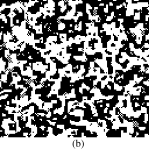
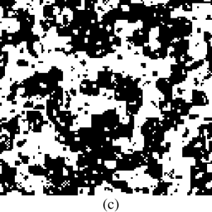
FIG. 1.: Snapshots of the coarsening process: positive (resp. negative) spins are represented by a black (resp. white) pixel on a two-dimensional grid. This simulation of the Miller-Huse model is performed at the critical point $g_{c}=0.20534$, for an initial magnetization $m_{0}=2.4\;10^{-4}$ ($m_{0}=2K/L^{2},K=2,L=128$). Snapshots $(a)$, $(b)$ and $(c)$ correspond to evolution times $t=0$ (completely disordered initial condition), $t=t_{\rm mic}=5$ (build-up of macroscopic correlations) and $t=T=128$ (“initial critical slip” regime).

The value of the critical coupling strength $g_{c}$ was previously obtained according to Binder’s method. We use $g_{c}=0.20534(2)$ [8]. As predicted in [13], a regime of initial growth of the magnetization is observed, as well as the crossover toward nonlinear relaxation for large enough initial magnetization $m_{0}$. The corresponding coarsening process is illustrated in Fig. 1. For measurement purposes, we use $K=2,4,6,8,10$, for sizes ranging between $L=16$ and $L=128$. The duration of a run is $T=128$. In such conditions, no crossover is observed to the nonlinear relaxation regime, since $t_{0}\gg T$. Thanks to the good quality of our data, the value of the microscopic time $t_{\rm mic}=5$ can be obtained by simple visual inspection (Fig. 2). This relatively small value is comparable to what has been observed for the two-dimensional Ising model [19]. Scaling of the magnetization versus time is observed over the time interval $5\leq t\leq 128$. This corresponds to the initial critical slip regime.

The exponent $\theta^{\prime}$ is measured thanks to a linear fit in log-log scale over the interval $t_{\rm mic}\leq t\leq T$. We checked that using larger values of $t_{\rm mic}$ and/or $T$ does not alter the estimate. Note also that using values of the critical coupling outside the confidence interval $g_{c}=0.20534(2)$ does not lead to an improved quality of fits: this confirms the validity of estimates of the critical coupling obtained in [8].

Ensemble averages are performed over $512000$ realizations for $L\leq 64$, $128000$ realizations for $L=128$. Statistical errors are estimated by comparing the exponent values obtained for five different initial magnetizations $m_{0}=2K/L^{2}$, $K=2,4,6,8,10$. Error bars take into account the uncertainty on $g_{c}$. Note that the corresponding values of $m_{0}$ are much smaller than those used by Okano et al., who needed to extrapolate exponent values obtained for small, but finite initial magnetization to the limit $m_{0}=0$. Our procedure is similar to that used by Grassberger [18], since no extrapolation is needed. The exponent values thus measured for $L=32,64,128$ are respectively $\theta^{\prime}=0.148(2),0.142(4)$ and $0.148(7)$. Statistically equivalent values are obtained when considering the magnetization based on the continuous variables. Within error bars, no finite-size effect is observed for $L\geq 32$. Our global (conservative) estimate is:

$$\theta^{\prime}_{\rm MH}=0.146(9).$$ (17)

Note that this result is not consistent with the accepted value for the critical dynamics of Model A: $\theta^{\prime}=0.193(6)$ obtained by similar methods and with a similar statistical quality in [18, 19].

FIG. 2.: Measure of the dynamic critical exponent $\theta^{\prime}$ for the Miller-Huse model. We plot in log-log scale the magnetization $M(t)$ vs. time $t$ measured at the critical point $g=g_{c}=0.20534$. Clear scaling is observed in all cases for $t\geq t_{\rm mic}=5$. The solid lines in both graphs correspond to a slope equal to $\theta^{\prime}=0.146$. Graph $(a)$: the system size $L=128$ is fixed, the initial magnetization $m_{0}=2K/L^{2}$ varies between $m_{0}=2.4\;10^{-4}$ and $1.2\;10^{-3}$, for $5$ distinct values of $K=2,4,6,8,10$ (from bottom to top). Good agreement between slopes corresponding to different values of $K$ suggests that the limit $m_{0}\rightarrow 0$ is satisfactorily approximated. Graph $(b)$: the initial condition $K=6$ is fixed, for system sizes $L=16,32,64,128$ (from top to bottom). Finite-size effects are negligible. This suggests that the infinite-size limit is satisfactorily approximated.

C Measure of $z$

A first way to measure exponent $z$ is given by Eq. 7. The experimental conditions are similar to those mentioned in the last section, but for an initial magnetization equal to zero ($m_{0}=0$, $K=0$). Simulations were performed for $L=16,32,64,128$, $T=128$, ensemble averages performed over $512000$ realizations for $L\leq 64$ and $128000$ realizations for $L=128$. Log-log plots of the second moment $M^{(2)}$ vs time show very good scaling, and lead to estimates of the combination of exponents $\zeta=(d-2\beta/\nu)/z=7/(4z)$, assuming that $\beta/\nu=1/8$ for $d=2$, as implied by [8]. In order to avoid interferences with the current experimental uncertainty on $\beta/\nu$ —estimated to be $\beta/\nu=0.131(6)$ in [8]—, we will work with $\zeta$, and convert into $z$ as late as possible. Longer runs (up to $T=1024$) were performed for large system sizes ($L=128$), with lesser statistical accuracy. This allowed to check that the exponents measured do indeed correspond to the asymptotic regime (cf. Fig. 3).

Here, determining the microscopic time $t_{\rm mic}$ requires additional effort, when compared to the previous case. We use a method introduced by Okano et al. [19]. Local exponents $\zeta(t)$ are first measured from “local” fits limited to an interval of time $[t,t+t_{\rm loc}]$. The microscopic time $t_{\rm mic}$ is defined as the time beyond which $\zeta(t)$ becomes stationary, within statistical fluctuations. We find $t_{\rm mic}\sim 30$, for $t_{\rm loc}=15$ and all sizes $L$ considered. This value does not depend on the value of $t_{\rm loc}$ for $t_{\rm loc}$ large enough. The microscopic time measured here is much larger than the one estimated for the scaling of $M(t)$ at small $m_{0}$, as had already been observed for the Ising model [19].

Asymptotic values of $\zeta$ are then obtained, as before, from a global linear fit performed in log-log scale over the interval $t_{\rm mic}\leq t\leq T=128$. As before, we checked that values obtained do not change, within error bars, for $15\leq t_{\rm mic}\leq 50$. Again, these values were independent on whether the discrete spins or the continuous variables were used to calculate the magnetization.

In this case, finite-size effects are sizeable and can be well controlled: we obtain values of $\zeta(L)$ for sizes $16\leq L\leq 128$ which are monotonously decreasing and seem to converge. Statistical errors are evaluated from a comparison of exponent values measured for three coupling strength values in the confidence interval $[0.20532,0.20536]$. As before, the quality of fits does not increase when varying $g_{c}$ outside this interval. In order to evaluate the rate of convergence, we use the Ansatz:

$$\zeta(L)-\zeta(\infty)\sim L^{-\omega},$$ (18)

where $\zeta(\infty)$ is the desired infinite-size exponent. Although algebraic relaxation toward an asymptotic value seems natural in the context of critical phenomena, we are not aware of any theoretical justification for Eq. 18. The validity of this phenomenological Ansatz is confirmed by our data (Fig. 3), which is not compatible with, e.g., exponential relaxation. Optimizing linear fits in log-log scale of $\zeta(L)-\zeta(\infty)$ vs. $L$ yields the following estimate: $\zeta(\infty)=0.839(3)$ (and, incidentally, $\omega=1.4$). The Ising value $0.817$ is not compatible with our data plus Ansatz 18 (see inserts of Fig. 3). Note that we use here the numerical results of [19] as a reference value for Model A. The discrepancy between our data for the Miller-Huse model and the currently accepted value [12] for Model A ($\zeta=0.808(6)$, see discussion in Sec. II) is even larger.

Using the theoretical, exact Ising value for $\beta/\nu$ [8], our estimate yields $z=2.082(4)$, at variance with the Model A exponent, irrespective of the method used to estimate it, whether it is initial critical slip [19, 20] or standard methods [12]. Using the measured value $\beta/\nu=0.131(6)$ [8], one obtains:

$$z_{\rm MH}=2.07(2),$$ (19)

a conservative estimate which we endorse.

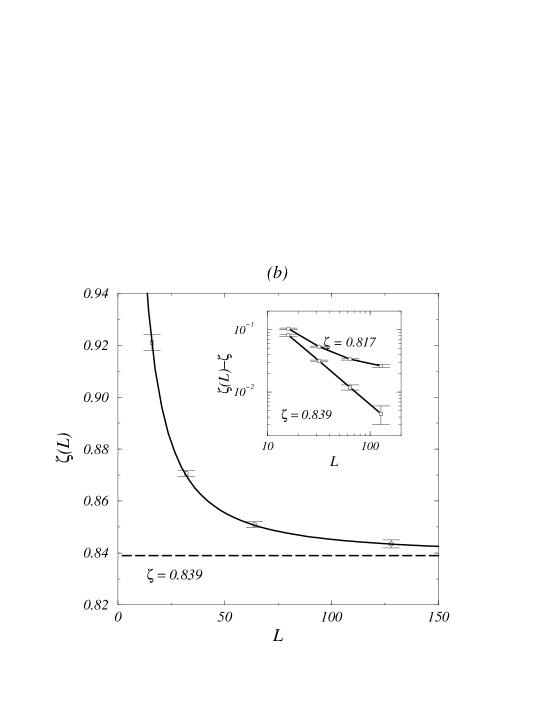
FIG. 3.: Measure of the dynamic critical exponent $z$ for the Miller-Huse model. Graph $(a)$: we plot in log-log scale the second moment $M^{(2)}(t)$ vs. time $t$ at the critical point $g=g_{c}=0.20534$, for an initial magnetization $m_{0}=0$. System sizes are $L=16,32,64,128$ (from top to bottom). Scaling is observed for $t\geq t_{\rm mic}\sim 30$. The solid line corresponds to a slope equal to $\zeta=(d-2\beta/\nu)/z=0.839$. The curves corresponding to $L=64$ and $L=128$ ($T=128$) are undistinguishable. This suggests that finite-size effects become small for $L\geq 64$. Data obtained for $L=128$, $T=1024$, $32000$ realizations (triangular symbols) shows no evidence of cross-over to a distinct time-asymptotic regime. Insert: we plot the ratio $M^{(2)}(t)/t^{\zeta}$ vs. time $t$ in log-lin scale for the values $\zeta=0.817$ (Model A, top curve) and $\zeta=0.839$ (best fit for extrapolated value in the infinite-size limit (see (b)), bottom curve). The system size is $L=128$, $T=128$. This graph shows that our (finite-size) data is not compatible with exponent values expected for Model A. Graph $(b)$: we plot the finite-size exponent $\zeta(L)$ vs. system size $L$, as obtained from linear fits of the data presented in Graph $(a)$ for $30\leq t\leq 128$. The infinite-size estimate $\zeta=\zeta(\infty)=0.839$ (dashed line) is derived from the relation $\zeta(L)=0.839+3.9L^{-1.4}$ (solid line). The insert shows a log-log plot of $\zeta(L)-\zeta(\infty)$ vs. system size $L$ for the two values $\zeta=0.817$ (Model A) and $\zeta=0.839$ (measured). The latter value optimizes the quality of a linear fit of $\log(\zeta(L)-\zeta)$ vs. $\log(L)$. This plot indicates that our data is not compatible with exponent values expected for Model A when extrapolated to the infinite-size limit.

Confirmation of the previously measured values may in principle be obtained from the scaling behavior of the correlation function (Eq. 8), with an exponent $\delta=d/z-\theta^{\prime}$. Previously measured values lead to $d/z-\theta^{\prime}=0.81(1)$. Even though the runs used are the same as for the second moment $M^{(2)}$, in practice, scaling is not satisfactory. In particular, local exponents $\delta_{\rm loc}(t)$ do not converge to stationary values. Very strong finite-size corrections to the dominant scaling are present, which preclude any effective measurement of $\delta$. However, the observed behavior is compatible with large-size, long-time convergence to the above value $\delta=d/z-\theta^{\prime}=0.81(1)$. Direct, reliable estimates for $\delta$ remain beyond our numerical resources.

In conclusion, the above study of the Miller-Huse model first shows that the regime of initial critical slip exists also for (some) deterministic systems, with the same phenomenology as for spin systems. Quantitatively, our simulations lead to the conclusion that the Miller-Huse model does not belong to the dynamic universality class of Model A. Since the mode of update is the relevant parameter explaining departure from the Ising universality for static critical exponents in this model [8], one would naturally like to know whether or not this is also true for dynamic exponents. Section IV deals with this question, with the study of two models with respectively sequential and checkerboard update.

IV Update rules

A Sequential update

The model considered here is identical to the Miller-Huse model except for one point: the update rule. Evolution rule 14 is replaced by:

$$x_{i,j}^{t+1}=(1-4g)\;f(x_{i,j}^{t})+g\;\left(f(x_{i-1,j}^{t+1})+f(x_{i,j-1}^{t+1}+f(x_{i+1,j}^{t})+f(x_{i,j+1}^{t})\right).$$ (20)

Sites are updated one at a time, in sequential order from the top, leftmost site to the bottom, rightmost one, as in:

$$\begin{array}[]{rl}\ldots\rightarrow&(1,1)\rightarrow(2,1)\rightarrow(3,1)\rightarrow\ldots\rightarrow(L,1)\rightarrow\\ \rightarrow&(1,2)\rightarrow(2,2)\rightarrow(3,2)\rightarrow\ldots\rightarrow(L,2)\rightarrow\\ &\ldots\\ \rightarrow&(1,L)\rightarrow(2,L)\rightarrow(3,L)\rightarrow\ldots\rightarrow(L,L)\rightarrow\ldots\end{array}$$ (21)

where arrows indicate the order of update between sites of indices $(i,j)$. Consequently, boundary conditions are helical in this case. (Note that this mode of update was termed “asynchronous” in [8].) A continuous transition similar to the Ising ferromagnetic point occurs in this system too, albeit for significantly lower coupling strength $g_{c}=0.11255(5)$, as measured in [8] thanks to Binder’s method. Its (measured) static critical exponents are compatible with the static Ising universality class $\beta/\nu=0.117(12)$, $\nu=1.02(7)$ [8].

FIG. 4.: Measure of the dynamic critical exponent $\theta^{\prime}$ in the case of sequential update. The magnetization $M(t)$, measured at the critical point $g=g_{c}=0.11255$, is plotted vs. time $t$ in log-log scale. Scaling is observed in all cases for $t\geq t_{\rm mic}=5$. The solid line in both graphs corresponds to a slope equal to $\theta^{\prime}=0.06$. Graph $(a)$: the system size $L=128$ is fixed, the initial magnetization $m_{0}=2K/L^{2}$ varies between $m_{0}=2.4\;10^{-4}$ and $1.2\;10^{-3}$, for values of $K=2,4,6,8,10$ (from bottom to top). Graph $(b)$: the initial condition $K=6$ is fixed, for system sizes $L=16,32,64,128$ (from top to bottom). Finite-size effects are negligible.

The initial conditions to measure the early-time critical properties of this transition are prepared as for the Miller-Huse model. The observed phenomenology is the same, for a comparable microscopic time $t_{\rm mic}\sim 5$, as estimated visually (Fig. 4). The value of $t_{\rm mic}$ is confirmed by the method described in Sec. III C (local exponent). Finite-size effects are negligible for $L\geq 32$. Measurement of the dynamic critical exponent $\theta^{\prime}$ is based on sizes $L=32,64,128$. The number of realizations over which ensemble-averaging is performed is the same as before, $512000$ for $L=32,64$, and $128000$ for $L=128$ (see Fig. 4). Our final estimate is

$$\theta^{\prime}_{\rm Sequential}=0.06(2).$$ (22)

Error bars take into account both statistical errors and the uncertainty due to the error bars on the location of the critical coupling strength. This is clearly not compatible with either the value obtained for the Miller-Huse model ($\theta^{\prime}=0.146(9)$) or with the Model A value ($\theta^{\prime}=0.193(5)$). At this stage we have no particular understanding of the low value of $\theta^{\prime}$ in this case. Finally, note that our data is equally well fitted by a logarithmic time-dependence: $M(t)\sim\log(t)$, for which no theoretical justification is at present available.

FIG. 5.: Measure of the dynamic critical exponent $z$ in the case of sequential update. The second moment of the magnetization $M^{(2)}(t)$ (graph $(a)$) and the temporal autocorrelation function $A(t)$ (graph $(b)$) are plotted in log-log scale vs. time $t$, as measured at the critical point $g=0.11255$, for zero initial magnetization $m_{0}=0$, up to time $T=2048$. The system sizes considered are $L=16,32,64,128$. All curves superpose for $M^{(2)}(t)$, and the last three for $A(t)$. The microscopic time $t_{\rm mic}$ can be roughly evaluated to $t_{\rm mic}={\cal O}(1000)$, especially from the inserts, where we plot in log-lin scale the local exponents $\zeta_{\rm loc}(t)$ and $\delta_{\rm loc}(t)$ vs. time $t$, computed for $L=64$, over time intervals of duration $t_{\rm loc}=100$. Graph $(a)$: the $\zeta$ values corresponding to Model A ($\zeta=0.817$, solid lines) and the Miller-Huse model ($\zeta=0.839$, dashed lines) are indicated. Graph $(b)$: the bottom and top curves respectively correspond to sizes $L=16$ and $L=32,64,128$ (superposed). The $\delta$ values corresponding to Model A ($\delta=0.74$, solid lines) and the Miller-Huse model ($\zeta=0.81$, dashed lines) are indicated. Note that fluctuations of $\zeta_{\rm loc}(t)$ and $\delta_{\rm loc}(t)$ observed for $t\geq t_{\rm mic}$ encompass the values for both models.

Measuring the exponent $z$ is much more difficult, since the microscopic time (or rather the time beyond which corrections to dominant scaling vanish and the asymptotic regime sets in) is very large, of the order of $t_{\rm mic}\sim 1000$. This is clearly shown in Fig.5, and in particular from the plots of the local exponents vs. time in the inserts. Ensemble averages are computed over typically $64000$ independent runs, for a simulation time of $T=2048$. Estimates of exponents must be derived from intervals much smaller than one decade (typically $1000\leq t\leq 2048$). Linear fitting in log-log scale is thus impractical. For that reason, we assume that the plateau observed for $t>t_{\rm mic}$ in plots of the local exponents correspond to the asymptotic value, and evaluate error bars from the variation of local exponent within that interval (Fig.5). We obtain:

$$\begin{array}[]{lcl}\zeta_{\rm Sequential}&=&0.83(6),\\ \delta_{\rm Sequential}&=&0.78(8).\end{array}$$ (23)

The estimated value of $\zeta$, close to that of the Miller-Huse model, leads to $z=2.12(15)$ (assuming $\beta/\nu=1/8$), with error bars large enough to include the uncertainty on the exponent of both Model A and Miller-Huse model. The estimated value of $\delta$ is closer to that of Model A, but is too imprecise to be exploited.

We are thus unable to give an estimate of $z$ which would decide between the values for the Model A, the Miller-Huse model, or an eventual third number. It is clear, though, that our estimate of exponent $\theta^{\prime}$ ($\theta^{\prime}=0.06(2)$) is not compatible with the values of either Model A ($\theta^{\prime}=0.193(5)$) or the Miller-Huse model ($\theta^{\prime}=0.146(9)$).

The above results confirm, at the dynamic level, those obtained in [8] for the static critical properties of Ising-like phase transitions in systems made of coupled chaotic maps: the mode of update is relevant. In [8], the static exponents of the sequential-update model studied above were measured to be, within numerical accuracy, those of the Ising model. The above results show that these two models have different dynamic exponents (at least $\theta^{\prime}$). Is this due to their mode of update and/or to other factors? In the next subsection, we introduce Sakaguchi’s model, a system of coupled chaotic maps designed to have exactly the static exponents of the Ising model, in order to further assess the relevance of the mode of update and that of the nature of the model for the dynamic scaling properties of Ising-like transitions.

B Checkerboard update

A few years ago, Sakaguchi introduced a system of coupled Bernoulli maps with an exponential coupling scheme and checkerboard update, which leads exactly to the Ising equilibrium Gibbs measure [9].

Two continuous variables, $x_{i,j}^{t}$ and $\Delta_{i,j}^{t}$ in $[-1,1]$, are defined on each site of a two-dimensional square lattice with periodic boundary conditions. Their evolution rule reads:

$$\begin{array}[]{lclll}x_{i,j}^{t+1}&=&{2\over 1+\Delta_{i,j}^{t}}\left(x_{i,j}^{t}+1\right)-1,&\;-1<x_{i,j}^{t}<\Delta_{i,j}^{t},\\ x_{i,j}^{t+1}&=&{2\over 1-\Delta_{i,j}^{t}}\left(x_{i,j}^{t}-1\right)+1,&\;\Delta_{i,j}^{t}<x_{i,j}^{t}<1,\end{array}$$ (24)

where the (time-dependent) slopes $\Delta_{i,j}^{t}$ of the Bernoulli maps are calculated according to:

$$\Delta^{t}_{i,j}=\mbox{tanh}\left\{J\left(\sigma_{i-1,j}^{t-1}+\sigma_{i+1,j}^{t-1}+\sigma_{i,j-1}^{t-1}+\sigma_{i,j+1}^{t-1}\right)\right\},$$ (25)

with $J$ a coupling constant. Discrete spin variables can be defined by:

$$\sigma^{t}_{i,j}=\mbox{sign}\left(x_{i,j}^{t+1}-x_{i,j}^{t}\right)\in\{-1,1\}\,,$$ (26)

which allows to retain definition 16 for the fluctuating magnetization.

When sites are updated successively on two checkerboard lattices defined by the parity of $i+j$, it is possible to show that the invariant measure of this system is the same as that of the Ising model [9]:

$$P^{\rm eq}\left(\{\sigma_{i,j}=m_{i,j}\}\right)\sim\exp\;J\left\{\sum_{i,j}m_{i,j}(m_{i-1,j}+m_{i+1,j}+m_{i,j-1}+m_{i,j+1})\right\}.$$ (27)

Therefore, static exponents are known exactly (Onsager solution). This was checked numerically in [8], following the same procedure as that used for the Miller-Huse model. Sakaguchi’s model does indeed belong to the Ising universality class for static critical exponents.

However, nothing is known a priori on dynamical properties, which we will investigate now along the same lines as before. One advantage of Sakaguchi’s model is that the critical point $J_{c}$ is known exactly. One source of error is thus eliminated. One drawback is the following: the magnetization $M$ depends on site values at two consecutive time steps. The method used previously in order to prepare initial conditions with fixed small initial magnetization cannot work. Instead, we applied the following procedure: start from random initial conditions and evolve the system at high temperature (at low $J_{\rm init}$, the system is in the disordered phase with zero mean magnetization) until it reaches by itself the desired initial magnetization $m_{0}$. The system is then quenched to the critical coupling. Since the magnetization is calculated from discrete spins, there is no dispersion on the value of initial conditions ($m_{0}=2K/L^{2}$, as before). Yet, this procedure is more costly numerically, which explains why, in the following, the obtained statistical accuracy is somewhat lower than for the previous two models studied here. In practice, we use $J_{\rm init}=0.1$, before quenching to $J_{c}=\ln(1+\sqrt{2})/2$.

The protocol used is the same as before. As expected, this model also exhibits a well-defined initial critical slip regime. In fact, the microscopic time $t_{\rm mic}$ turns out to be equal to $0$ (Fig.6). A possible explanation for this is that the macroscopically-correlated domains present at $J_{\rm init}$ survive the quench to $j_{c}$. Impeccable scaling is observed for the initial growth of the magnetization $M$. Reliable measurements are possible only for $L=32$ and $64$: cross-over to the nonlinear relaxation regime occurs too soon ($t_{0}\sim 60$) for $L=16$, and $L=128$ is too costly to reach satisfactory statistical quality due to the preparation of initial conditions. Ensemble average is done over $128000$ realizations simulated during $T=128$ timesteps. From linear fits over the full interval $0\leq t\leq 128$, we obtain $\theta^{\prime}=0.197(7)$ for $L=32$ and $0.19(1)$ for $L=64$ (Fig.6). Within error bars, no finite-size effects are present. Our estimate is:

$$\theta^{\prime}_{\rm Sakaguchi}=0.194(14),$$ (28)

in good agreement with results obtained for Model A [18, 19], and not consistent with the value obtained for the Miller-Huse model.

FIG. 6.: Measure of the dynamic critical exponent $\theta^{\prime}$ for Sakaguchi’s model. The magnetization $M(t)$, measured at the critical point $J=J_{c}$ (cf. text), is plotted vs. time $t$ in log-log scale. In both graphs, the solid line corresponds to a slope equal to $\theta^{\prime}=0.193$ (Model A). Graph $(a)$: the system size $L=32$ is fixed, while the initial magnetization $m_{0}=2K/L^{2}$ varies between $m_{0}=7.8\;10^{-3}$ and $9.8\;10^{-3}$, for values of $K=4,6,8,10$ (from bottom to top). The microscopic time $t_{\rm mic}$ is equal to zero. Scaling is thus observed over more than two decades. Graph $(b)$: the initial condition $K=4$ is fixed, for system sizes $L=16,32,64$ (from top to bottom). The crossover time for the smallest size $L=16$ is observable: $t_{0}\sim 60$. Finite-size effects are negligible for $L=32,64$.

Again, measuring $z$ is more difficult. The scaling of $M^{(2)}$ starts late, with a fairly large microscopic time ($t_{\rm mic}\sim 40$ for $L=64$, $t_{\rm mic}\sim 70$ for $L=128$), estimated as before from the evolution of local exponents. As for non-zero initial magnetizations, ensemble average is performed over $128000$ realizations, and the simulation time is $T=128$, for system sizes up to $L=128$. Exponents are thus estimated over less than one decade. However, finite-size effects are negligible for $L\geq 32$. We obtain:

$$\zeta_{\rm Sakaguchi}=0.82(2)$$ (29)

(note the large error bars). From the exact value $\beta/\nu=1/8$, this leads to: $z=2.13(5)$, roughly compatible with both Model A and the Miller-Huse model. A longer simulation time ($T=1024$), even for the largest system size ($L=128$) leads to qualitatively identical results, without any quantitative improvement: the insert of Fig. 7.a shows that fluctuations of the local exponent $\zeta_{\rm loc}$, computed over time intervals of duration $t_{\rm loc}=100$, include values of $\zeta$ expected for both Model A and the Miller-Huse model.

The situation concerning the scaling behavior of the time autocorrelation function is somewhat more satisfactory, despite (or thanks to) finite size effects: large size behavior converges toward a value of $\delta$ which is necessarily smaller than the Miller-Huse exponent $\delta=0.81(1)$. In fact, data obtained for the largest size considered ($L=128$, $T=128$) is characterized by a scaling exponent $\delta=d/z-\theta^{\prime}\sim 0.75$, compatible with Model A value $\delta=0.74(1)$ (cf. Fig. 7.b). This finding is confirmed qualitatively by runs performed for longer simulation times ($L=128$, $T=2048$): the Miller-Huse value is not allowed by the evolution of effective behavior (exponent) with system size. Since we cannot cross-check with larger system size due to numerical limitations, we do not provide error bars on our estimate:

$$\delta_{\rm Sakaguchi}\sim 0.75.$$ (30)

FIG. 7.: Measure of the dynamic critical exponent $z$ for Sakaguchi’s model. The second moment of the magnetization $M^{(2)}(t)$ (graph $(a)$) and the temporal autocorrelation function $A(t)$ (graph $(b)$) are plotted in log-log scale vs. time $t$, as measured at the (exact) critical point $J=J_{c}$. for zero initial magnetization $m_{0}=0$, up to time $T=128$. The system sizes considered are $L=16,32,64,128$, for $128000$ realizations. Graph $(a)$: finite-size effects become negligible for $L\geq 32$. The solid and dashed lines respectively correspond to slopes equal to $\zeta=0.817$ (Model A) and $\zeta=0.839$ (Miller-Huse model). In the insert, we plot the local exponent $\zeta_{\rm loc}(t)$ computed over intervals $t_{\rm loc}=100$, for $L=128$, $T=1024$, data averaged over $32000$ realizations. Fluctuations of $\zeta_{\rm loc}(t)$ encompass both values expected for Model A and the Miller-Huse model. Graph $(b)$: the slope of the solid line is equal to $-\delta=-0.74$ (Model A). The insert shows, for $L=128$, a log-lin plot of the ratio $A(t)/t^{-\delta}$ vs. time $t$ for the numerical values $\delta=0.74$ (Model A, bottom curve) and $\delta=0.81$ (Miller-Huse model, top curve). This suggests that the continuous transition of Sakaguchi’s model belongs to the universality class of Model A for the exponent $\delta$.

Our numerical results show clearly that the critical dynamics of Sakaguchi’s model belongs neither to the universality class of Miller-Huse model, nor to that of the sequentially updated model studied in Sec. IV A. It is moreover likely that Sakaguchi’s model belongs to the universality class of Model A, for both statics and dynamics: the checkerboard update of Sakaguchi’s model may thus be analogous to that of, say, Glauber dynamics of a spin system.

Our results may be summarized as follows (see Table I for numerical values of all exponents estimated so far): update is a relevant parameter for dynamic critical exponents of Ising-like transitions of coupled chaotic map systems. Not only models with static exponents outside the Ising universality class (Miller-Huse) have also their dynamic exponents different from those of Model A, but models within the Ising static class (sequentially-updated Miller-Huse, Sakaguchi) may also have non-Ising dynamic exponents (sequentially-updated Miller-Huse). In some sense, this is not too surprising since update is already known to be a relevant parameter for the dynamical exponents of spin systems in the Ising static class. In the next section, we go a step further and investigate whether the universality found at the static level in [8] among synchronously-updated CMLs subsists at the dynamic level.

V Non-universality within synchronously-updated models

In this section, we study two variants of the Miller-Huse model: we consider first the case of a locally anisotropic coupling to three neighbors, and then the case where the piecewise linear local map (13) is replaced by a smooth map. The static exponents $\beta$, $\gamma$ and $\nu$ of these variants were measured to be the same, within error bars, as those of the Miller-Huse model. Given the difficulties encountered above when trying to estimate the exponent $z$, in this section we restrict ourselves to measurements of the exponent $\theta^{\prime}$, via the early-time scaling of $M(t)$.

The three-neighbor variant of the Miller-Huse model was studied in [8] because of its particularly weak corrections to scaling. Its anisotropic evolution rule reads:

$$\left\{\begin{array}[]{lcl}x_{2i,j}^{t+1}&=&(1-3g)\;f(x_{2i,j}^{t})+g\;\left(f(x_{2i-1,j}^{t})+f(x_{2i+1,j}^{t}+f(x_{2i,j+1}^{t})\right),\\ x_{2i+1,j}^{t+1}&=&(1-3g)\;f(x_{2i+1,j}^{t})+g\;\left(f(x_{2i,j}^{t})+f(x_{2i+2,j}^{t}+f(x_{2i+1,j-1}^{t})\right),\end{array}\right.$$ (31)

where $f$ is the original piecewise linear map (13). Each site is thus coupled to three of its nearest neighors: sites belonging to even (resp. odd) columns of the lattice are coupled vertically to their northern (resp. southern) neighbor only. Rule (31) is applied synchronously to all sites, with periodic boundary conditions. The local anisotropy introduced vanishes at large scales. In this case, an Ising-like transition takes place for a critical coupling $g_{c}=0.25118(4)$, estimated using Binder’s method [8].

The smooth map variant only differs from the Miller-Huse model by the choice of the local function $f$, which remains a chaotic, odd map of the $[-1,1]$ interval for symmetry reasons, but now reads:

$$f(x)=3x-4x^{3}\;.$$ (32)

On general grounds, this smooth function, with its expanding and contracting parts, may be considered more “generic” than the original piecewise linear map. An Ising-like transition also takes place in this case, for a slightly smaller critical coupling than the Miller-Huse model: $g_{c}=0.17864(4)$ [8].

For both variants, hereafter referred to as “MH3” (three-neighbor coupling) and “C4” (smooth cubic map), the methodology used in Sec. III to determine exponent $\theta^{\prime}$ for the original Miller-Huse model can be applied. Initial conditions with fixed, small magnetization $m_{0}$ are prepared using the same procedure, and the phenomenology observed is the same. In both cases, the microscopic time is visually estimated to be $t_{\rm mic}\sim 5$. After this time, a clear scaling behavior is observed for $M(t)$ (Fig. 8). Sizes $L=16$, 32, 64 and 128 were studied, with ensemble-averaging over 512000 realizations for $L\leq 64$ and 128000 for $L=128$. Finite-size effects are smaller than error bars for $L\geq 32$. Statistical errors on $\theta^{\prime}$ are estimated by comparing values obtained for different initial magnetization $m_{0}=2K/L^{2}$ with $K=2,4,8$ and coupling strengths $g$ within the uncertainty interval of $g_{c}$. Our global (conservative) estimates are:

$$\theta^{\prime}_{({\rm MH3})}=0.165(8)\;\;\;\;{\rm and}\;\;\;\;\theta^{\prime}_{({\rm C4})}=0.128(6)\;.$$ (33)

Not only these values are not compatible with each other, but both are also at odds with the value found for the original Miller-Huse model ($\theta^{\prime}=0.146(9)$).

FIG. 8.: Measure of the dynamic critical exponent $\theta^{\prime}$ for two variants of the Miller-Huse model. The magnetization $M(t)$, measured at the critical coupling $g_{c}$ (cf. text), is plotted vs. time $t$ in log-log scale. The system size is $L=64$ (top three curves on each graph), and $L=128$ (bottom two curves, shifted down for clarity). The initial magnetization is $m_{0}=2K/L^{2}$. The microscopic time $t_{\rm mic}$ is equal to 5. Graph $(a)$: anisotropic three-neighbor coupling with original piecewise linear local map (13) (model MH3). The solid lines correspond to slopes equal to $\theta^{\prime}=0.165$. From bottom to top: $L=128$, $K=8,16$ and $L=64$, $K=2,4,8$. Graph $(b)$: symmetric four-neighbor coupling with smooth cubic local map (32) (model C4). The solid lines correspond to slopes equal to $\theta^{\prime}=0.128$. From bottom to top: $L=128$, $K=8,16$ and $L=64$, $K=3,4,8$.

Numerical estimates of $\theta^{\prime}$ obtained for all models we considered are gathered in Table II. Except in the presence of finite-size and finite-time effects not detectable in the experimental conditions of our work, the above results lead to conclude that CMLs of the Miller-Huse type exhibit different exponents for the dynamic critical properties of their Ising-like transitions even though they share the same static exponents and the same mode of update.

VI Discussion

The first conclusion about the series of numerical experiments conducted in this work is that non-trivial early-time critical dynamics occurs in phase transitions of far from equilibrium, coupled map lattices. The microscopic time $t_{\rm mic}$ after which scaling sets in tends to be small for $M(t)$, generally of the same order of magnitude as for equilibrium systems. On the other hand, $t_{\rm mic}$ is typically at least one order of magnitude larger for the evolution of second-order quantities such as $M^{(2)}(t)$ and $A(t)$. This is also in agreement with spin systems [19]. One would however like to understand why $t_{\rm mic}$ is always larger for second-order quantities than for $M(t)$. Intuitively, it can be argued that in order for the scaling regime of $M^{(2)}(t)$ and $A(t)$ to set in, the system first needs to generate macroscopically-correlated regions, i.e. $M(t)$ must already be in its scaling regime. Thus $t_{\rm mic}(M^{(2)}(t),A(t))\geq t_{\rm mic}(M(t))$. Further, one may argue that macroscopically-correlated regions for second order quantities can only establish themselves when the magnetization $M(t)$ has changed “significantly”, say by a factor 2. Using $M(t)\sim t^{\theta^{\prime}}$, one obtains $t_{\rm mic}(M^{(2)},A(t))\sim 2^{1/{\theta^{\prime}}}$. This admittedly rough argument may explain semi-quantitatively why microscopic times observed for the Miller-Huse models with sequential and synchronous update differ by two orders of magnitude: $t_{\rm mic}({\rm Seq.})/t_{\rm mic}({\rm MH})\sim 2^{(1/0.06)-(1/0.146)}\sim 2^{10}$, or $1024$. In addition, finite-size corrections to scaling are also typically much larger for second-order quantities than for $M(t)$. A direct consequence of the observed values of $t_{\rm mic}$ and of the strength of finite-size corrections is that, in practice, the exponent $\theta^{\prime}$ is much easier to measure than the exponent $z$, our initial goal. Thus, although $z$ remains largely out of reach in some cases, the critical initial slip method offers the advantage of accurate estimations of $\theta^{\prime}$.

The second conclusion of our work lies in the interpretation of the various dynamic exponent values we measured, which are summarized in Tables I and II.

First, and perhaps most importantly, we confirm, at the level of dynamic critical properties, the results obtained in [8] at the static level: update is a relevant parameter for universality classes of Ising-like transitions. Synchronously-updated coupled map models —such as the Miller-Huse model and its variants MH3, C4— have critical exponents different from those of Model A both at the static and dynamic level. For the original Miller-Huse model, our data is even conclusive for both exponents $\theta^{\prime}$ and $z$.

Secondly, we extend to the transitions of coupled chaotic maps a result already known for equilibrium spin systems: the static universality class of the Ising model breaks down at the dynamic level. The sequentially-updated Miller-Huse model and the Sakaguchi model, which are in the static Ising class, possess different dynamic exponents (in fact our data is unambiguous only for $\theta^{\prime}$). The distinction between checkerboard and sequential update is known to be irrelevant at equilibrium for both static and dynamic critical exponents, including the exponent $\theta^{\prime}$ [18, 19]. However, the same distinction becomes relevant at the dynamic level for lattices of coupled chaotic maps. An additional interesting point is that Sakaguchi’s model seems to possess the dynamic exponents $\theta^{\prime}$ and $z$ of Model A.

Thirdly, our data gathered for the sole exponent $\theta^{\prime}$ indicates the splitting of the “non-equilibrium universality class” for the static critical properties of synchronously-updated coupled map systems showing Ising-like transitions. Variants of the Miller-Huse model, all shown in [8] to share the same static exponents, exhibit different values of $\theta^{\prime}$. Again, as for spin systems, universality classes are narrower for dynamical critical exponents than for static ones. Excluding Sakaguchi’s model, whose control parameter is too markedly different to allow a meaningful comparison, one may notice that numerical estimates of $\theta^{\prime}$ for the four other models depend monotonously on the critical coupling $g_{c}$ (see Table II): lower values of the coupling constant correspond to a slower coarsening process. We believe this can be understood by considering the structure of the phase space of these systems which can be seen as a hierarchy of repellors. During coarsening, this hierarchy is explored, and thus its scaling properties — which probably depend on $g$ — must be related to the scaling behavior which defines $\theta^{\prime}$. Of course, the above picture will need to be substantiated in the future, but it already suggests a link between the structure of the phase space (and hence the details of the dynamics) and exponent $\theta^{\prime}$.

In agreement with our findings, which confer a sort of “maximal” non-universality to $\theta^{\prime}$, the tentative picture sketched above, invites comments on the relative status of $z$ and $\theta^{\prime}$. Unfortunately, our attempts at measuring $z$ (via $\zeta$ and $\delta$) have largely failed, mainly because of large values of $t_{\rm mic}$. However, data obtained for the variants C4 and MH3 of the Miller-Huse model are compatible with the idea of a greater universality for $z$ than for $\theta^{\prime}$. In particular, they suggest that variant C4 might possess the same $z$ value as the original Miller-Huse model. Thus, we would like to suggest that $\theta^{\prime}$ may be considered as a quantity highly dependent on the details of the dynamics in non-equilibrium situations, while $z$, in comparison, is a more global quantity. The independence of exponents $z$ and $\theta^{\prime}$ is consistent with this conjecture.

To summarize, our numerical experiments provide additional contradictory evidence to the conjecture of [3] in the case of continuous phase transitions of coupled chaotic map systems. In other words, the qualitative features of scaling are correctly predicted by renormalization-group methods (since, e.g., the scaling behavior predicted by [13] is observed), but the same techniques fail to predict exponents quantitatively. The above remarks, though, call for more detailed investigations of the respective role of the various dynamical exponents involved in order to explain the origin of the non-universality reported here. In particular, the possibly different status of $z$ and $\theta^{\prime}$ provides an interesting starting point on which to base further research, at both the numerical and theoretical levels. Further, one would also like to know whether the various persistence exponents defined and studied recently for spin systems [23] —and particularly the “global persistence” exponent defined in [24]— also pertain to continuous phase transitions of chaotic coupled map lattices, and if so, whether their numerical value also depends on the fine details of the coarsening process following uncorrelated initial conditions, similarly to the dynamic exponent $\theta^{\prime}$. This is the subject of ongoing research.

	Model A	Miller-Huse	Sequential	Sakaguchi
Critical point	$\ln(1+\sqrt{2})/2$	$0.20534(2)$	$0.11255(5)$	$\ln(1+\sqrt{2})/2$
$\theta^{\prime}$	$0.193(5)$	$0.146(9)$	$0.06(1)$	$0.194(14)$
$\zeta=(d-2\beta/\nu)/z$	$0.808(6)$	$0.839(3)$	$0.83(6)$	$0.82(2)$
$z$	$2.165(15)$	$2.07(2)$	$2.12(15)$	$2.13(5)$
$\delta=d/z-\theta^{\prime}$	$0.74(1)$	No estimate	$0.78(8)$	$\sim 0.75$

TABLE I.: Update is a relevant parameter for dynamic critical exponents: a summary of numerical estimates of the dynamical exponents $\theta^{\prime}$, $\zeta$, $z$ (obtained from $\zeta$) and $\delta$, for three models with synchronous (Miller-Huse model, Sec. III), sequential (Sec. IV A), and checkerboard (Sakaguchi’s model, Sec. IV B) update. The exponent values given for Model A are discussed in Sec. II. Number(s) in brackets correspond to the uncertainty on the last(s) digit(s), e.g. $0.193(5)$ means $0.193\pm 0.005$,

	2D Ising	Sakaguchi	Sequential	C4	Miller-Huse	MH3
Static universality class	Ising	Ising	Ising	Synchronous	Synchronous	Synchronous
Critical point	$\ln(1+\sqrt{2})/2$	$\ln(1+\sqrt{2})/2$	$0.11255(5)$	$0.17864(4)$	$0.20534(2)$	$0.25118(4)$
$\theta^{\prime}$	$0.193(5)$	$0.194(14)$	$0.06(1)$	$0.128(6)$	$0.146(9)$	$0.165(8)$

TABLE II.: The universality observed for the static properties of Ising-like transitions of lattices of coupled chaotic maps does not hold for their dynamic critical properties: a summary of numerical estimates of the dynamical critical exponents $\theta^{\prime}$. Number(s) in brackets correspond to the uncertainty on the last(s) digit(s), e.g. $0.193(5)$ means $0.193\pm 0.005$,