A condition for the genotype–phenotype mapping: Causality

Abstract

The appropriate choice of the genotype $\rightarrow$ phenotype mapping in combination with the mutation operator is important for a successful evolutionary search process. We suggest a measure to quantify the quality of this combination by addressing the question whether the relation among distances is carried over from one space to the other. Search processes which do not destroy the neighbourhood structure are termed strongly causal. We apply the proposed measure to parameter and structure optimisation problems in order to assess the combination (mapping, mutation operator) and at the same time to be able to propose improved settings.

published in:
T. Bäck (Ed.) (1997) Proceedings of the Seventh International Conference on Genetic Algorithms (ICGA’97), Morgan Kauffman, 73-80.

1 Introduction

The optimisation process in evolutionary algorithms is largely influenced by the mapping from the genotype space to the phenotype space. Especially for structure optimisation problems a measure of the quality of the combination (mapping, mutation, crossover) would be desirable. In this paper we propose such a measure based upon the observation that Darwinian evolution takes gradual changes to the optimum, although in biological evolution other phenomena like punctuated equilibria are also observed.

We demand that the search process is locally strongly causal with respect to the mutation operator, that is: small variations on the genotype space due to mutation imply small variations in the phenotype space. This way the neighbourhood structure under the mapping ${\cal G}\rightarrow{\cal P}$ is conserved, see Figure 1. The distance on the genotype space is defined via the mutation probability. The need for a strong causal exploration of the search space has been expressed before [Rechenberg 1994, Lohmann 1993]. However, in the following we want to quantify the degree to which the setting (mapping, mutation operator) satisfies the causality condition.

The distance measure and therefore the causality condition in section 2 only depends on the mutation and not on the crossover operator. This does not represent any opinion whether one or the other is the driving force in evolutionary algorithms. However, we believe that the mutation operator usually is responsible for small steps in the phenotype space, hence for gradual changes which we want to analyse. Furthermore, we assume a locally smooth fitness function and define conditions for the genotype $\rightarrow$ phenotype mapping for this problem domain. Thus, unlike in correlation based analysis, [Jones et al. 1995, Manderick et al. 1991], we do not explicitly refer to a fitness landscape, instead we focus on the conservation of neighbourhood structures.

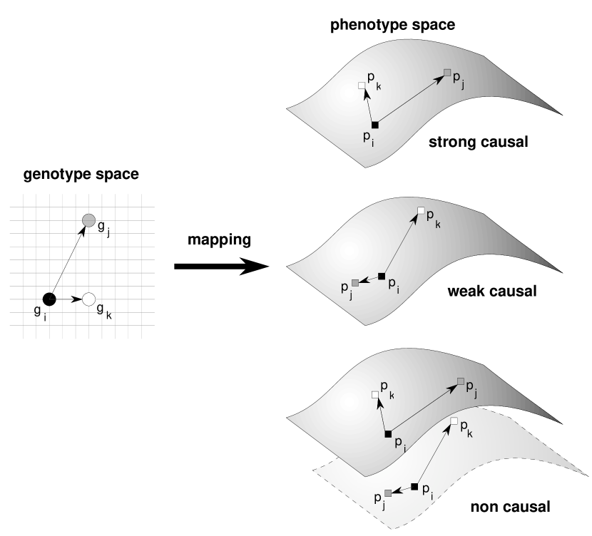
Figure 1: Examples for strongly, weakly and non causal genotype–phenotype mappings under the influence of mutation. Circles denote genotypes $(g_{i},g_{j},g_{k})$, $g_{j}$ and $g_{k}$ are results of mutations from $g_{i}$. The corresponding phenotypes $(p_{i},p_{j},p_{k})$ are shown as squares. The first strongly causal mapping does not destroy the neighbourhood structure in genotype space, the second weakly causal mapping, maps small mutations in genotype space to large distances in phenotype space and vice versa. The last example shows a non-causal mapping.

In the next section we will propose a condition for a strongly causal search process and quantify it by introducing a probabilistic interpretation of the condition. Section 3 presents a first application in the domain of parameter optimisation problems and the following section is concerned with the structure optimisation of neural networks, where complicated genotype $\rightarrow$ phenotype mappings are commonly used.

2 A Condition for Causality

In section 1 we claim that for the successful introduction of new information by mutation the mutation operator should preserve the neighbourhood structure in the corresponding evolutionary spaces. We believe that strong causality is necessary in evolutionary algorithms

• to allow for controlled small steps in the phenotype space which are provoked by small steps in the genotype space. Especially in the vicinity of an optimum we need small steps to gradually approach the optimum.

• for the ability of self-adaptation of any strategy parameters, since with the lack of strong causality the information about the past is meaningless and adaptation is impossible.

In order to formulate the causality condition we have to define the term small variation in a mathematical sense. Therefore, we introduce a measure of distance in the genotype and phenotype space. For the mathematical correctness we have to show that the measure in the respective spaces endows these spaces with a metric. For distances in the genotype space we propose a “universal” measure which is based on the probability of reaching genotype $g_{j}$ from genotype $g_{i}$. In this respect it resembles definitions of distance used in evolutionary biology, [Schuster 1995a]: “…the notion of distance in genotype space is given by the smallest number of individual mutations required for the interconversion of two genotypes …”. Furthermore, this measure is general enough to be applicable to a wide range of evolutionary algorithms.
We introduce the following notations: Genotype space ${\cal G}=\{g_{i}\}$ and phenotype space ${\cal P}=\{p_{i}\}$. Both ${\cal G}$ and ${\cal P}$ can also be continuous spaces. The mapping between the spaces is $f:{\cal G}\mapsto{\cal P}$, thus $p_{i}=f(g_{i})$. The operators mutation and crossover act upon the space ${\cal G}$, the selection operator acts upon the fitness space ${\cal F}$ and therefore on ${\cal P}$. We parameterise the mutation operator by a real valued vector $\vec{\sigma}\in{I\hskip-3.0ptR}^{l}$.

Now, we will introduce the definition of distance on ${\cal G}$, based on the mutation probability $P(g_{i}\!\stackrel{{\scriptstyle\vec{\sigma}}}{{\rightarrow}}\!g_{j})$ of reaching $g_{j}$ from $g_{i}$ in ${\cal G}$ via mutation which is characterised by $\vec{\sigma}$.

$$d(g_{i},g_{j}) = -\log\left(\frac{1}{P_{id}}\,P(g_{i}\!\stackrel{{\scriptstyle\vec{\sigma}}}{{\rightarrow}}\!g_{j})\right)$$ (1)

$$P_{id} = P(g\!\stackrel{{\scriptstyle\vec{\sigma}}}{{\rightarrow}}\!g)$$ (2)

This definition is only sensible if we claim that $P(g_{i}\!\stackrel{{\scriptstyle\vec{\sigma}}}{{\rightarrow}}\!g_{j})<P_{id}$ and that the probability not to mutate is independent of $g$, which is satisfied by most evolutionary algorithms. The logarithm in eq. (1) is introduced in order to make the distance measure additive instead of multiplicative. The properties of this measure are discussed in [Sendhoff et al. 1997].

Eq. (1) allows for the comparison between different EAs independent of any particular metric on the genotype space, like Hamming distance or Euclidian distance.

Now, we can proceed with the definition of causality.

Condition: Strong causality

$\displaystyle\forall g_{i},g_{j},g_{k}\;\;\exists\vec{\sigma^{\prime}},\varepsilon\leavevmode\nobreak\ \leavevmode\nobreak\ \mbox{with}\leavevmode\nobreak\ \leavevmode\nobreak\ \vec{\sigma}\in U_{\varepsilon}(\vec{\sigma^{\prime}})$

$$||f(g_{i})-f(g_{j})||<||f(g_{i})-f(g_{k})||$$ (3)

$$\Longleftrightarrow -\log\!\left(\frac{P(g_{i}\!\!\stackrel{{\scriptstyle\vec{\sigma}}}{{\rightarrow}}\!\!g_{j})}{P_{id}}\right)<-\log\!\left(\frac{P(g_{i}\!\!\stackrel{{\scriptstyle\vec{\sigma}}}{{\rightarrow}}\!\!g_{k})}{P_{id}}\right)$$

$$\Longleftrightarrow P(g_{i}\!\stackrel{{\scriptstyle\vec{\sigma}}}{{\rightarrow}}\!g_{j})>P(g_{i}\!\stackrel{{\scriptstyle\vec{\sigma}}}{{\rightarrow}}\!g_{k})$$

The additional condition that $\vec{\sigma}$ can be drawn from anywhere inside a sphere with radius $\varepsilon$ ($\varepsilon$ can be sufficiently small) around $\vec{\sigma^{\prime}}$ guarantees that the effect of mutation continuously varies with $\vec{\sigma}$. That is, besides the existence of an appropriate $\vec{\sigma}$, we have to guarantee that it is possible to locate. Mathematically, the space of all mutation parameters which satisfy the causality condition is not empty and additionally not of measure zero.

We have indicated, that our analysis is concerned with the local behaviour of evolutionary search. Therefore, condition (3) should not be seen as a global condition. The term local is difficult to define. However, an absolute measure of locality is not necessary since we are interested in the relative performance of EAs.

Condition (3) defines strong causality in both directions. Small distances and variations on the phenotype space imply small distances and variations in the genotype space with respect to the probability of jumping this distance via mutation and vice versa. However, in most EAs the second direction is more important. That is, small variations in the genome provoke small variation in the phenotype.

So far we have only set up a qualitative condition for strong causality. In order to compare between EAs, we have to find a quantitative version of condition (3). We will rephrase it in the light of a probabilistic interpretation.

Assuming the $g_{i},g_{j},g_{k}$ to be random variables with uniform distribution, both sides of condition (3) become boolean random variables. As a shortcut, we introduce the symbols $A$ and $B$:

$$A := ||f(g_{i})-f(g_{j})||<||f(g_{i})-f(g_{k})||$$ (4)

$$B := -\log\!\left(\frac{P(g_{i}\!\!\stackrel{{\scriptstyle\vec{\sigma}}}{{\rightarrow}}\!\!g_{j})}{P_{id}}\right)<-\log\!\left(\frac{P(g_{i}\!\!\stackrel{{\scriptstyle\vec{\sigma}}}{{\rightarrow}}\!\!g_{k})}{P_{id}}\right)$$ (5)

$$\Longleftrightarrow B\;:=\;P(g_{i}\!\stackrel{{\scriptstyle\vec{\sigma}}}{{\rightarrow}}\!g_{j})>P(g_{i}\!\stackrel{{\scriptstyle\vec{\sigma}}}{{\rightarrow}}\!g_{k})$$

Since we assume the distribution of $g_{i},g_{j},g_{k}$ to be known, we can derive the probabilities $P(A)$, $P(B)$, and $P(A,B)$. We can now, with the help of Bayes’ law, recast the two directions (genotype $\leftrightarrow$ phenotype) in the following way:

Probabilistic condition: Strong causality

$\displaystyle\forall g_{i},g_{j},g_{k}\;\;\exists\vec{\sigma^{\prime}},\vec{\varepsilon}\leavevmode\nobreak\ \leavevmode\nobreak\ \mbox{with}\leavevmode\nobreak\ \leavevmode\nobreak\ \vec{\sigma}\in U_{\varepsilon}(\vec{\sigma^{\prime}})$

$${\cal G}\Rightarrow{\cal P}:\leavevmode\nobreak\ \leavevmode\nobreak\ P(A|B) = \frac{P(A,B)}{P(B)}\,=\,1$$ (6)

$${\cal P}\Rightarrow{\cal G}:\leavevmode\nobreak\ \leavevmode\nobreak\ P(B|A) = \frac{P(A,B)}{P(A)}\,=\,1$$ (7)

The value of $P(A|B)$ serves as a quantitative measure for the causality in EAs. If the neighbourhood relations in both spaces are uncorrelated for every point, then the system is weakly but not strongly causal $P(A,B)=P(A)\cdot P(B)$ and therefore $P(A|B)=P(A)$, $P(B|A)=P(B)$, thus distance relations in the phenotype space are statistically independent from distance relations in the genotype space and vice versa. One example for such systems is the class of Monte Carlo algorithms where the transition probability between any pair of genotypes is constant. For constant transition probabilities, $B$ in equation (5) is constant for all genotype combinations and does therefore not provide any information about the distance relation in the phenotype space.

In evolutionary molecular biology measures similar to this probabilistic formulation of the causality condition are employed in the context of the analysis of the “sequence–structure” mapping [Schuster 1995b].

3 Parameter Optimisation

Firstly, we employ one of the mainstream paradigms of EAs – the evolution strategy (ES) and show that the ES is strongly causal in terms of our proposed condition. As an example for an EA, which violates the causality condition, we analyse the canonical genetic algorithm (GA) applied to parameter optimisation. We propose a new mutation operator for the GA which observes strong causality to a greater extent and show that this also increases the performance.

3.1 Evolution Strategy

We firstly focus on the transition probability. In the canonical ES ${\cal G}\!=\!{\cal P}\!=\!{I\hskip-3.0ptR}^{n}$ and the genotype $\rightarrow$ phenotype mapping is the identity $f:{\cal G}\rightarrow{\cal P}$ $={\mbox{id}}_{{I\hskip-3.0ptR}^{n}}$. It uses normally distributed mutation steps which are independent of the genotype $g_{i}\in{\cal G}$. That is, the transition $g_{i}\!\stackrel{{\scriptstyle\vec{\sigma}}}{{\rightarrow}}\!g_{k}$ is defined by adding a normally distributed number $z=(z_{1},\dots,z_{n})$ with $z_{i}\sim N(0,\sigma^{2})$. Hence, the pdf of this transition can be expressed in terms of $z$

$$g_{i}\!\!\stackrel{{\scriptstyle\vec{\sigma}}}{{\rightarrow}}\!\!g_{k} : g_{j}=g_{i}+z$$ (8)

$$p(g_{i}\!\!\stackrel{{\scriptstyle\vec{\sigma}}}{{\rightarrow}}\!\!g_{k}) = p(z=g_{j}-g_{i})$$ (9)

$$= \frac{1}{\sqrt{2\pi}^{\,n}\sigma^{n}}\exp\!\left(\!-\frac{\|g_{k}\!\!-\!\!g_{i}\|^{2}}{2\sigma^{2}}\!\right)$$

$$p_{id} = p(z=0)\leavevmode\nobreak\ =\leavevmode\nobreak\ \frac{1}{\sqrt{2\pi}^{\,n}\sigma^{n}}$$ (10)

Inserting the transition pdf in the causality condition (3) with $f:{\cal G}\rightarrow{\cal P}={\mbox{id}}_{{I\hskip-3.0ptR}^{n}}$ results in

$$\|f(g_{i})-f(g_{j})\|<\|f(g_{i})-f(g_{k})\|$$ (11)

$$\Longleftrightarrow \|g_{i}-g_{j}\|<\|g_{i}-g_{k}\|$$

$$\Longleftrightarrow \exp\left(-\|g_{i}-g_{j}\|^{2}\right)>\exp\left(-\|g_{i}-g_{k}\|^{2}\right)$$

$$\Longleftrightarrow p(g_{i}\!\!\stackrel{{\scriptstyle\vec{\sigma}}}{{\rightarrow}}\!\!g_{j})>p(g_{i}\!\!\stackrel{{\scriptstyle\vec{\sigma}}}{{\rightarrow}}\!\!g_{k})$$

which holds for all combinations of $g_{i},g_{j},g_{k},\sigma$.

The examination of the metric conditions of the distance measure of an ES and some notes on the self-adaptation of $\sigma$ are presented in [Sendhoff et al. 1997].

3.2 Genetic Algorithms

In the case of genetic algorithms (GA) the genotype space consists of binary strings of length $L$, therefore ${\cal G}=\{0,1\}^{L}$. Canonical GAs mutate by changing each bit position from $0\rightarrow 1$ and $1\rightarrow 0$, respectively, with the probability $p_{m}$. Thus, $p_{m}$ corresponds to the mutation parameter $\sigma$. Let $h_{ij}$ denote the Hamming distance between $g_{i}$ and $g_{j}$.

In order to examine the causality condition we use the Euclidian metric on the phenotype space ${\cal P}$ and choose the standard binary coding for the genotype–phenotype mapping $f:{\cal G}\rightarrow{\cal P}$. Using the following notations

$$g_{i} = \{x_{i}(n)\,|\,x_{i}(n)\in\{0,1\}\}$$ (12)

$$h_{ij} = \sum_{n=0}^{L-1}\left|x_{i}(n)-x_{j}(n)\right|$$ (13)

$$f(g_{i}) = \sum_{i=0}^{L-1}x_{i}(n)\,2^{n}$$ (14)

$$P(g_{i}\!\stackrel{{\scriptstyle\vec{\sigma}}}{{\rightarrow}}\!g_{j}) = p_{m}^{h_{ij}}(1-p_{m})^{L-h_{ij}}$$ (15)

the causality condition is expressed as

$$\displaystyle\left|\sum_{n=0}^{L-1}(x_{i}(n)\!-\!x_{j}(n))\,2^{n}\right|<\left|\sum_{n=0}^{L-1}(x_{i}(n)\!-\!x_{k}(n))\,2^{n}\right|$$

$$\displaystyle\Longleftrightarrow\leavevmode\nobreak\ p_{m}^{h_{ij}}(1\!-\!p_{m})^{L\!-\!h_{ij}}>p_{m}^{h_{ik}}(1\!-\!p_{m})^{L\!-\!h_{ik}}\leavevmode\nobreak\ \leavevmode\nobreak\ \leavevmode\nobreak\$$ (16)

Assuming $p_{m}<0.5$ the right hand side of (16) can be expressed as $h_{ij}<h_{ik}$. Therefore the causality condition reads

$$\displaystyle\left|\sum_{n=0}^{L-1}(x_{i}(n)\!-\!x_{j}(n))\,2^{n}\right|<\left|\sum_{n=0}^{L-1}(x_{i}(n)\!-\!x_{k}(n))\,2^{n}\right|$$

$$\displaystyle\Longleftrightarrow\leavevmode\nobreak\ \sum_{n=0}^{L-1}\left|x_{i}(n)\!-\!x_{j}(n)\right|<\sum_{n=0}^{L-1}\left|x_{i}(n)\!-\!x_{k}(n)\right|\leavevmode\nobreak\ \leavevmode\nobreak\ \leavevmode\nobreak\ \leavevmode\nobreak\ \leavevmode\nobreak\ \leavevmode\nobreak\$$ (17)

which obviously does not hold in general, not even locally.

As a measure of the extent to which the GA satisfies the causality condition we employ the probabilistic version of the condition. After some extensive calculations which are presented in [Sendhoff et al. 1997] we get $P(A|B)\approx 0.51$ and $P(B|A)\approx 0.62$. That is, the chance of a small mutation of a genotype resulting in a small change of the corresponding phenotype is about 51%. The probability that a small change of a phenotype is caused by a small mutation of the genotype is somewhat higher, about 62%. Thus, in the case of a canonical GA, the mapping from the genotype to the phenotype is not strongly causal. In our opinion the combination of binary coding and point mutation is not well suited for continuous parameter optimisation combined with locally smooth fitness functions and is the reason why ES, which observes strong causality, outperforms the GA in most cases in this problem domain.

3.3 A New Mutation Operator

We have seen that in GA the standard mutation operator together with the binary encoding does not satisfy the causality condition in general. Possible solutions to this problem are to use a different encoding scheme, e.g. the Gray code, to change the mutation operator and keep the encoding scheme, and to change both.

In the remainder of this section we will partly outline an approach, presented in detail in [Sendhoff et al. 1996], which sticks to the concept of point mutation, but uses a position dependent mutation rate $p_{m}=p_{m}(i)$. This will provide us with an interesting example of an EA, where a modification of the mutation operator enhances the causality and, as we will see, also the performance.

Figure 2: Top: $p_{m}(i)$ for $\sigma=10.0$ (dashed curve - numerical approximation), bottom: $p_{m}(i)$ (rescaled with a factor 8) for $\sigma=0.5$ (dashed curve - numerical approximation).

As we have seen above, the ES is a strongly causal optimisation procedure. Therefore, we translate the concept of mutation by adding normally distributed numbers in ES to point mutation in GAs. Thus, we calculate a probability distribution which will on average resemble the summation of a normally distributed number. Depending on the standard deviation $\sigma$ of the underlying normal distribution we get different distributions of the mutation rates $p_{m}(i)$, see Figure 2. For the efficient use of the new mutation operator we derived a numerical approximation of $p_{m}(i;\sigma)$ which is presented in [Sendhoff et al. 1996].

(a)

(b)

Figure 3: Convergence plots of optimisation runs. The solid line shows the results obtained by position-dependent mutations. Dashed lines the ones from the canonical GA. (population size: 50; dimension: $n=30$; encoding length: 32 bits using Gray-code)

The numerical estimates of the causality measure are $P(A|B)\approx 0.73$ and $P(B|A)\approx 0.74$. In order to support our hypothesis that increasing the strong causality in an optimisation process leads to an improved performance we apply the modified GA to two standard optimisation problems. Results are given for the sphere model and Ackley’s function, see figure 3. The new GA converges faster to a better value than the canonical GA. Figure 3 shows that in case of the sphere model the increase of convergence speed is of order $10^{5}$ and for the Ackley function of order $10^{1.5}$.

4 Causality in Structure Optimisation

The problem to choose the right genotype $\rightarrow$ phenotype mapping is of particular importance in the domain of structure optimisation. We will here concentrate on the structure optimisation of neural networks. We will regard the set of all possible connection matrices as the phenotype space, and allow the matrix to have entries from $\{0,1\}$ or from $\{0,...,N_{sym}\}$. Since there is no measure on the space of these matrices which relates directly to the performance of the neural network without evaluating the network, we will use the standard Euclidian distance measure for the phenotype space, ($y_{nk}^{M_{j}}$ denotes the entry at (row $n$, column $k$) of the matrix $M_{j}$)

$$d_{E}(M_{i},M_{j})=\frac{1}{N^{2}}\sum_{n=1}^{N}\sum_{k=1}^{N}|y_{nk}^{M_{i}}-y_{nk}^{M_{j}}|$$ (18)

There is no a priori structure assumed for the network, hence the matrix is not constrained to any layered network structure. If $y_{nk}>0$ there exists a connection between neuron $n$ and neuron $k$. We are not restricted to the upper triangular part of the matrix, thus in principle feedback connections can be specified. If the $y_{nk}$ are restricted to the values $\{0,1\}$, we only specify the connection between the neurons. If we extend the allowed values to all integers in the set $\{0,...,N_{sym}\}$, it is possible to further define initial values for the weights and the thresholds. In connection with gradient descent algorithms for the fine tuning of the weights, this approach has been successful, see [Sendhoff et al. 1997], and we will therefore include it in the following examinations.

There have been several proposals on how to organise the genotype space and the mapping $f:{\cal G}\rightarrow{\cal P}$ for the optimisation of the structure of neural networks, see also [Whitley 1995]. Most of them can be categorised into three principal approaches, the direct encoding, the recursive or grammar encoding and the cellular encoding. The first attempts to use evolutionary (genetic) algorithms for structure optimisation employed the direct encoding method, [Miller et al. 1989], and it probably still is the most frequently used method. The recursive encoding has been introduced by Kitano (?), in order to overcome the bad scaling behaviour of the direct encoding method for large networks and to favour a modular structure of the network. The third approach, the cellular encoding, proposed by Gruau (?), uses a tree representation of operators which construct the network. The structure of the tree and therefore of the network is optimised by genetic programming. In the following we will examine the direct encoding and the recursive encoding with respect to the proposed measure, eqs. (6, 7). Therefore, we will examine whether the neighbourhood structure on ${\cal G}$ is carried over to ${\cal P}$; whether the system is strongly causal. We will restrict ourselves to the direction, ${\cal G}\rightarrow{\cal P}$ and we will not sample uniformly in ${\cal G}$. The reason is, that for the mutation operator $p_{\pm}$ (see eq. (21)) the probability to reach the genotype $g_{j}$ and $g_{k}$ from $g_{i}$ is zero for almost all uniformly sampled triples. Thus, if we want to examine the system (mapping, $p_{\pm}$), we sample $g_{i}$ uniformly and obtain $g_{j}$ and $g_{k}$ via mutation from $g_{i}$ with the probability $p_{init}$. By tuning $p_{init}$, we are at the same time able to determine how local the three chromosomes are. We then derive the probability to reach $g_{j}$ and $g_{k}$ from $g_{i}$ by “normal mutation”.

4.1 The direct encoding method

In the direct encoding method the chromosome consists of the whole connection matrix. Usually all matrix rows are concatenated to form the chromosome, whose elements we want to denote by $x_{n}$. The range of allowed values for $x$ and $y$ can be $\{0,1\}$ or from the integer set $\{0,...,N_{sym}\}$. The following operators ($\chi\in[0,1[$ is a uniformly sampled number) have been used

$$p_{\pm}x = \left\{\begin{array}[]{lrl}x+1&;&\chi<0.5\\ x-1&;&\chi\geq 0.5\end{array}\right.$$ (21)

$$p_{u}x = \left\lfloor\chi\cdot(N_{sym}+1)\right\rfloor$$ (22)

$p_{u}$ replaces $x$ by a new integer with equal probability from the set $\{0,...,N_{sym}\}$. We used the Euclidian measure of distance for matrices on the phenotype space and a distance measure which only counts structural differences $d_{I}(M_{i},M_{j})$

$$\displaystyle d_{I}(M_{i},M_{j})=\frac{1}{N^{2}}\sum_{n=1}^{N}\sum_{k=1}^{N}|\Theta(y_{nk}^{M_{i}})-\Theta(y_{nk}^{M_{j}})|\leavevmode\nobreak\ \leavevmode\nobreak\ \leavevmode\nobreak\ \leavevmode\nobreak\$$ (23)

$$\Theta(x)=\left\{\begin{array}[]{lrl}0&;&x\leq 0\\ 1&;&x>0\end{array}\right.$$ (26)

The results for the probability $P(A|B)$, that is the probability that ($d_{E,I}$ denotes $d_{E}$ or $d_{I}$)

$$A:=d_{E,I}(M_{i},M_{j})>d_{E,I}(M_{i},M_{k})$$ (27)

holds in phenotype space, given that

$$B:=-\log\left(P(g_{i}\rightarrow g_{j})\right)>-\log\left(P(g_{i}\rightarrow g_{k})\right)$$ (28)

is true in genotype space, are presented in Table 1.

	$d_{E}$/$p_{\pm}$	$d_{I}$/$p_{\pm}$	$d_{E}$/$p_{u}$	$d_{I}$/$p_{u}$
$x\in\{0,1\}$	–	–	–	0.0
$x\in\{0,..,N_{sym}\}$	0.0	0.614	0.662	0.564

Table 1: Numerical estimation of the probabilities $P(A|B)$, using combinations of the two different distance measures and mutation operators. The probabilities have been estimated from $10^{5}$ trials ($N_{sym}=10$ and $p_{init}=0.25$).

The standard setting, $(x\in\{0,1\},d_{I},p_{u})$ is strongly causal in the ${\cal G}\rightarrow{\cal P}$ direction. However, if the allowed values are extended to an interval of integers, all settings have problems at least for the structural distance measure. Thus, we conclude that even direct encoding methods are not strongly causal straightforwardly if we depart from the basic setting.

4.2 The recursive encoding method

In all encoding methods apart from the one discussed above a more or less intrinsic mapping is introduced from the genotype to the phenotype space. We already argued why this is sensible and we now want to examine to what extent a recursive encoding method is strongly causal. The coding, described in [Sendhoff et al. 1997], consists of four chromosomes, where only the first two are important for the building process of the connection matrix. In each iteration step every element of the connection matrix is replaced by a $2\times 2$ matrix of new elements. The new elements are specified by a mapping from the small chromosome $S_{C}$ to the large chromosome $L_{C}$. The length of the small chromosome $N_{S_{C}}$ is variable, the length of the large one is fixed by the condition $N_{L_{C}}=4\cdot N_{S_{C}}$. At each step $i$ the first place $N(y_{nk}^{i})$ of each connection matrix element $y_{nk}^{i}$ in $S_{C}$ is determined; for example position $N(y_{1}=7)=3$ in Figure 4. The element is then replaced by the four elements at the positions

$$\displaystyle\big{(}\;4\cdot(N(y_{nk}^{i})-1)+1,\;4\cdot(N(y_{nk}^{i})-1)+2,\leavevmode\nobreak\ \leavevmode\nobreak\ \leavevmode\nobreak\ \leavevmode\nobreak\ \leavevmode\nobreak\ \leavevmode\nobreak\$$

$$\displaystyle 4\cdot(N(y_{nk}^{i})-1)+3,\;4\cdot(N(y_{nk}^{i})-1)+4\;\big{)}\leavevmode\nobreak\ \leavevmode\nobreak\$$ (29)

in the large chromosome $L_{C}$.

Figure 4: One element is replaced by four elements in the recursion step via the small chromosome $S_{C}$ $\rightarrow$ large chromosome $L_{C}$ mapping.

Figure 4 shows the replacement of an element $y_{1}=7$ by the four elements $\left(3,6,9,1\right)$. In case $y_{nk}^{i}$ is not in $S_{C}$, it is replaced by four so called terminal symbols (in the notation of integer strings, the most convenient choice is zero). A terminal symbol is in turn always replaced by another four terminal symbols in an recursion step. Figure 5 shows the evolution of a $8\times 8$ connection matrix $M_{con}$ following the introduced rules.

Figure 5: Scheme of the recursive development of the connection matrix up to a size of $8\times 8$.

This network connection matrix is a function of the mutation and crossover probabilities, the chromosome length $d_{S_{C}}$, the number of iteration steps $N_{steps}$ and of the size of the set of integers $\{1,...,N_{sym}\}$ of allowed values for both strings.

(a)

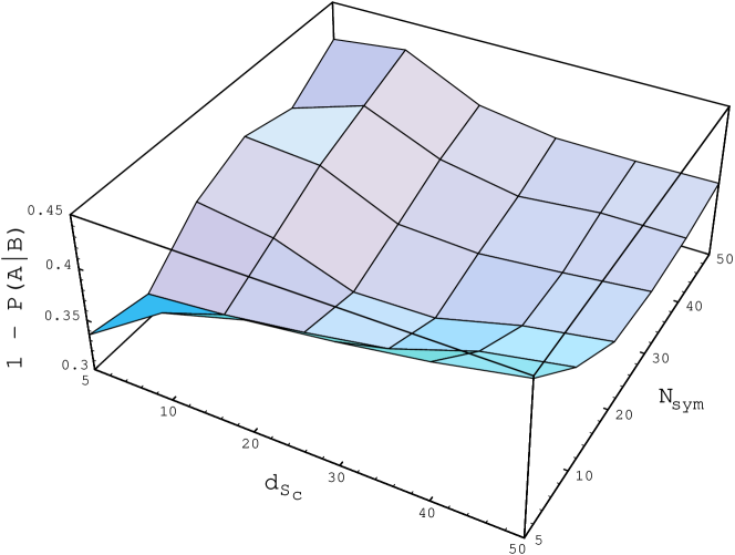
(b)

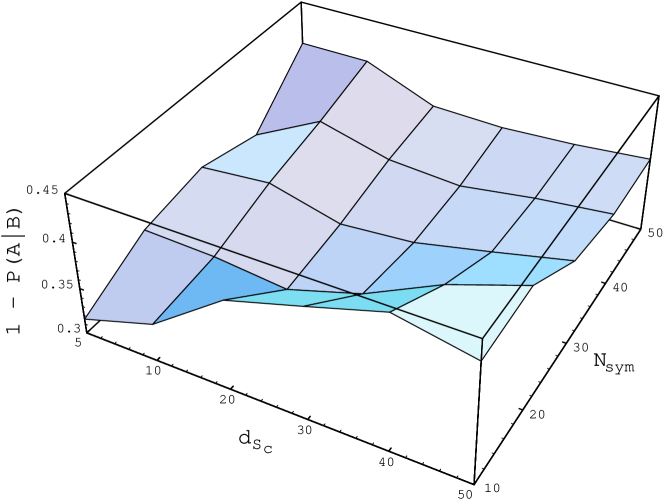
Figure 6: Since it is easier to visualise, the probability to violate the causality condition $(1-P(A|B))$ is shown for the (a) Euclidian distance measure $d_{E}$ and (b) structure distance measure $d_{I}$. The values have been estimated from $10^{5}$ trials ($p_{init}=0.25$).

We restrict ourselves to mutations on $S_{C}$ and examine the probability $(1-P(A|B))$ as a function of $d_{S_{C}}$ and $N_{sym}$, the results are shown in Figure 6 (a) for the Euclidian distance measure $d_{E}(M_{i},M_{j})$ and in (b) for the structure distance measure $d_{I}(M_{i},M_{j})$. Only the results for the $p_{\pm}$ mutation operator are shown, because the values for $p_{u}$ are only slightly lower and show a similar behaviour as in Figure 6. We note that the system is generally not strongly causal, especially for specific combinations ($d_{S_{C}},N_{sym}$). Furthermore, the best (lowest, since causality violations are shown) values on average are reached if the encoding parameters $d_{S_{C}}$ and $N_{sym}$ differ only slightly, thus we conclude $d_{S_{C}}\approx N_{sym}$. We also note that the differences between $d_{E}$ and $d_{I}$ are only marginal both qualitatively and quantitatively. Thus, from the point of view of causality the combined optimisation of the structure and the initial weight values seems to be sensible.

We will now, similar to section 3 in the domain of parameter optimisation, try to lower the probability of causality violations with the help of a new position dependent mutation operator. Firstly, we have to identify typical settings which are responsible for causality violations. One is a direct consequence of the redundant nature which from the viewpoint of accumulated mutation is also advantageous. Hence, we do not try to change the encoding to be less redundant, but instead we change the mutation operator, so that the mutation probability rises for redundant chromosome entries. If $p_{m}$ is the probability to mutate and $N_{x_{k}(S_{C})}$ denotes the number of occurrences of symbol $x_{k}(S_{C})$ in $S_{C}$ before the position of $x_{k}(S_{C})$, we write

$$p_{m}(x_{k}(S_{C}))=p_{m}\cdot(N_{x_{k}(S_{C})}+1)$$ (30)

Secondly, we observe that all elements from $S_{C}$ which occur in the first four elements in $L_{C}$ have a large impact on the connection matrix, since the first element in $S_{C}$ is always mapped onto this first block of elements in $L_{C}$. Therefore, we suggest a second modification to the mutation operator:

$$p_{m}(x_{k}(S_{C})) = p_{m}^{2}$$

$$\forall\;x_{k}(S_{C}) \in \{x_{1}(L_{C}),\ldots,x_{4}(L_{C})\}$$ (31)

Figure 7 (a) and (b) show the results for the probability of causality violating steps for the mutation operator with the modifications eqs. (30, 4.2) compared to the fixed mutation (dashed curve) rate $p_{m}$. In Figure 7 (a) we kept $N_{sym}$ constant and changed the length of $S_{C}$, since we expect that in this case modification (30) will have the largest impact because the amount of redundant elements in $S_{C}$ rises with $d_{S_{C}}$. Indeed, we observe that $(1-P(A|B))$ is considerably reduced and that the effect is more pronounced for larger values of $d_{S_{C}}$. Figure 7 (b) shows experiments carried out for the combinations $N_{sym}=d_{S_{C}}$ which, as we pointed out earlier, are the best choices for the coding parameters. The new mutation operator reduces the probability of causality violations also in these cases, however the difference to the fixed mutation rate is smaller than in Figure 7 (a). Thus, we conclude that minor modifications of the mutation operator can already have an causality enhancing effect on the search process and that it is worthwhile to analyse the (genotype $\rightarrow$ phenotype, mutation) system with respect to the question why and for which specific settings problems can occur.

(a)

(b)

Figure 7: The probability to violate the causality condition $(1-P(A|B))$ (see also Fig. 6) estimated from $10^{5}$ trials. (a) $N_{sym}=10$ is kept constant and (b) the relation $N_{sym}=d_{S_{C}}$ is fixed. The interlaced curve shows the values for the mutation operator with the modifications (30, 4.2) and the dashed curve for the standard mutation rate $p_{m}$ ($p_{init}=0.25$).

5 Conclusion

In this paper we suggested a condition which the setting (genotype $\rightarrow$ phenotype mapping, mutation) should fulfill in order to allow gradual changes for a local search on the phenotype space which can be controlled via the mutation parameter on the genotype space. We applied the probabilistic causality condition to problems in the domain of parameter optimisation and structure optimisation both analytically and constructively. Thus, besides examining the search process, we also suggested variations in the mutation operator to improve the setting with respect to our condition. Especially in the later domain, where complicated mappings are commonly used, we believe the measure could be a useful tool for constructing evolutionary algorithms. In the case of parameter optimisation, Figures 3 show that the setting which enhances the causal behaviour at the same time improves the performance.

Acknowledgements

This research work is part of the BMBF SONN project under Grant No. 01IB401A9.

References

- Gruau 1993 Gruau, F. (1993). Genetic synthesis of modular neural networks. In S. Forrest (Ed.), Proc. 5th Int. Conf. Genetic Algorithms, pp. 318–325. Morgan Kaufmann.
- Jones et al. 1995 Jones, T. and S. Forrest (1995). Fitness distance correlation as a measure of problem difficulty for genetic algorithms. In L. Eshelman (Ed.), Proc. 6th Int. Conf. Genetic Algorithms, pp. 184–192. Morgan Kaufmann.
- Kitano 1990 Kitano, H. (1990). Designing neural networks using genetic algorithms with graph generation system. Complex Systems 4, 461–476.
- Lohmann 1993 Lohmann, R. (1993). Structure evolution and incomplete induction. Biol. Cybern. 69(4), 319–326.
- Manderick et al. 1991 Manderick, B., M. de Weger, and P. Spiessens (1991). The genetic algorithm and the structure of the fitness landscape. In R. Belew and L. Booker (Eds.), Proc. 4th Int. Conf. Genetic Algorithms, pp. 143–150. Morgan Kaufmann.
- Miller et al. 1989 Miller, G. and P. Todd (1989). Designing neural networks using genetic algorithms. In D. Schaffer (Ed.), Proc. 3rd Int. Conf. Genetic Algorithms, pp. 379–384. Morgan Kaufmann.
- Rechenberg 1994 Rechenberg, I. (1994). Evolutionsstrategie ’94. Friedrich Frommann Holzboog.
- Schuster 1995a Schuster, P. (1995a). Artificial life and molecular evolutionary biology. In F. Moran et al. (Eds.), Advances in Artificial Life, pp. 3–19. Springer.
- Schuster 1995b Schuster, P. (1995b). How to search for RNA structures - theoretical concepts in evolutionary biotechnology. J. Biotechnology 41, 239–257.
- Sendhoff et al. 1996 Sendhoff, B. and M. Kreutz (1996). Analysis of possible genome–dependence of mutation rates in genetic algorithms. In T. Fogarty (Ed.), Evolutionary Computing, Volume 1143 of LNCS, pp. 257–269. Springer.
- Sendhoff et al. 1997 Sendhoff, B. and M. Kreutz (1997). Evolutionary optimization of the structure of neural networks using a recursive mapping as encoding. In Proc. 3rd Int. Conf. Artificial Neural Networks and Genetic Algorithms. Springer.
- Sendhoff et al. 1997 Sendhoff, B., M. Kreutz, and W. von Seelen (1997). Causality and the analysis of evolutionary algorithms. Submitted to IEEE Trans. Evolutionary Computation.
- Whitley 1995 Whitley, L. (1995). Genetic algorithms and neural networks. In J. Periaux and G. Winter (Eds.), Genetic Algorithms in Engineering and Computer Science, Chapter 11. John Wiley.