Evolution and extinction dynamics in rugged fitness landscapes.

Abstract

After an introductory section summarizing the paleontological data and some of their theoretical descriptions, we describe the ‘reset’ model and its (in part analytically soluble) mean field version, which have been briefly introduced in Letters[1, 2]. Macroevolution is considered as a problem of stochastic dynamics in a system with many competing agents. Evolutionary events (speciations and extinctions) are triggered by fitness records found by random exploration of the agents’ fitness landscapes. As a consequence, the average fitness in the system increases logarithmically with time, while the rate of extinction steadily decreases. This non-stationary dynamics is studied by numerical simulations and, in a simpler mean field version, analytically. We also consider the effect of externally added ‘mass’ extinctions. The predictions for various quantities of paleontological interest (life-time distribution, distribution of event sizes and behavior of the rate of extinction) are robust and in good agreement with available data.

1 Introduction and background

Life on earth originated 3.5 billion years ago. According to the earliest record of life, the first organisms were primitive one-celled non-photosynthesizing bacteria. Two billion years then followed, before more complex multicelled organisms appeared in a catastrophic event called the Cambrian explosion. This evolutionary event, which took place about 600 million years ago, led to a diversity of new species, and to a remarkable fossil record for the following Phanerozoic period, which provides valuable and fundamental material for scientists who seek insight into the fascinating history of life on earth.

Unfortunately, the fossil record is often limited when it comes to understanding the development of a given species at the level of organisms, i.e. the micro-evolutionary processes. However, the record makes out a good statistical material at the macro-evolutionary level, where species and higher taxa are the basic units considered[3]. At this and higher taxonomical levels, evolutionary measures, as for instance the distribution of life spans, provide a good characterization of biological evolution and a basis for understanding its underlying mechanism.

The evolution of species is typically sketched in the form of evolutionary trees with several lineage branchings. Whenever a lineage branches, it marks the appearance of new species (speciation), and whenever it stops, it marks the extinction of a species. We note that almost all species are extinct[4]. The possibility of hybridization, where two lineages merge to form a new intermediate species, is normally not seen. Other evolutionary changes are essential, the most prominent being the phyletic transformations taking place along a lineage. These transformations are basically Darwinian changes in species due to natural selection. The extinctions associated with phyletic transformations are called pseudo-extinctions.

Several questions arise when this Darwinian picture of evolution is taken under closer scrutiny. Did species always have time to adapt to the changes in their environment? And what are the selection mechanisms ( if any ) that on a species level determine who is to survive and who is to go extinct? Is evolution mostly characterized by gradual changes, or is it rather characterized by ‘quantal jumps’ or ‘punctuations’, where new species are formed on a relatively short geological time scale?

We may further ask: can evolution be described by dynamical processes fluctuating around fix values, or is there a sense of direction in biological evolution, expressed, for example, by a steadily increasing fitness measure? Why should nature select an average life time for species to be four million years? Why not four thousand years or 4 billion years?

Explanations of evolutionary and extinction history can be coarsely classified according to their standing on the question of gradualism, to the importance they confer to ‘bad luck’ as opposed to ‘bad genes’[5], and finally according to their view on stationarity. All these issue have been intensely debated by paleontologist. From fossil data, it seems to us that nature has indeed not selected an equilibrium. For example, the standing diversity of families of marine vertebrates[6] has increased by a large factor over the last 600 million years while, in the same period, the body plan complexity ( the number of different somatic cells in the most complex of the taxa extant at a given time ) has increased sixhundredfold[7]. The extinction rate does not appear to have reached an equilibrium either. Rather it seems to have a downward trend, as noted by Raup and Sepkoski[6] in 1982. Their data are reproduced in Fig. 1a. The decay of extinction intensity can be highlighted by integrating the extinction rate, measured as a percent of standing diversity. The accumulated extinction rate percent describes the number of extinctions in a (hypothetical) system with a constant standing diversity. If evolutionary dynamics were a stationary process, with – on average – an equal number of events taking place in any given time interval, this quantity would increase linearly in time. Instead, as shown in Fig. 1b, it increases as a power law $R(t)=t^{1-\gamma}$, and, correspondingly, the percentual rate of extinction $r(t)$ decays as $t^{-\gamma}$. The numerical value of $\gamma$ is $\approx 0.4$. Admittedly, the extinction record shows large fluctuations. The events which fall outside the expected statistical variation[8] are mainly related to the five big mass extinctions, which have attracted enormous interest, presumably due to their catastrophic impact on the ecosystem. The now most commonly accepted explanation of these events are meteor impacts[9].

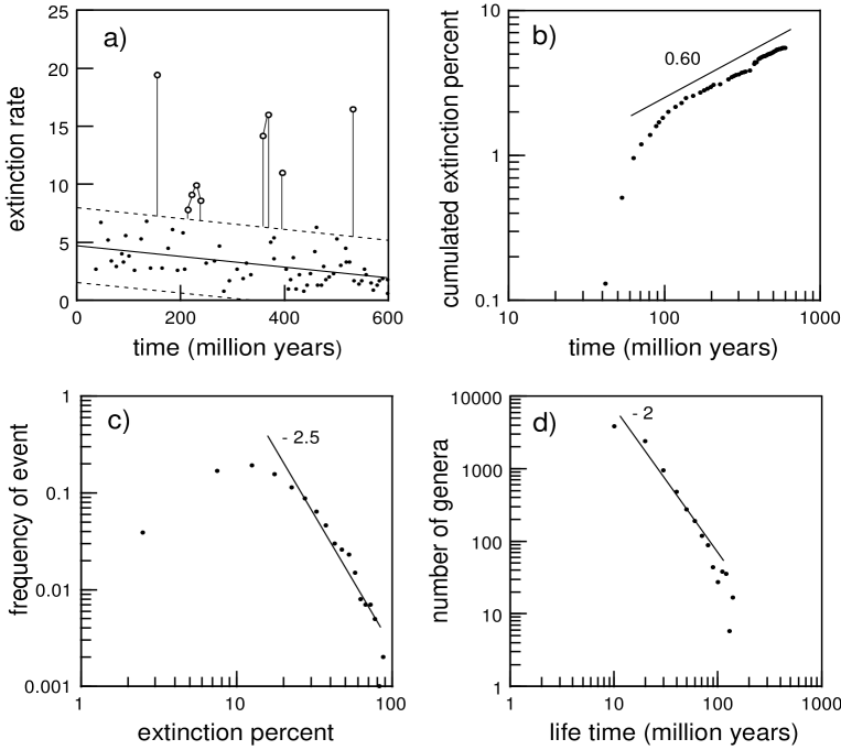
Figure 1:

a) The extinction rate (extinction per million years) for families of marine vertebrates and invertebrates is plotted as a function of geological time. These data are redrawn from Ref.[6]. b) Using the information on the corresponding standing diversity available from the same source, the extinction rate is converted in an extinction percentage, which is then integrated and shown in a log-log plot as a function of time. If extinction were a stationary process, this cumulative extinction percentage should fall on a line with slope $1$. Instead, as highlighted in the plot, the majority of data points fall on a line with slope $0.6$. In plots a) and b) the origin of time is set to $600$ million years ago, corresponding to the beginning of the Phanerozoic period. c) The shown data describe the distribution of extinction event sizes, expressed as fraction of the extant species killed. The data are redrawn from Ref. [4]. As shown in the figure the distibution of event sizes falls off approximately as a power law. The exponent is $-2.5$, which, as we argue in the text, is the reciprocal of the exponent characterizing the decay of the rate of extinction.

Meteor craters have been looked for and identified to account not only for the mass extinctions but also for several minor events, where a diversity of species seems to suddenly disappear within a short geological time span. However, since mass extinctions only represent a small fraction of the data, they only exert a relatively minor influence on the extinction rate.

An intriguing result of the decay of the extinction rate is its direct influence on other evolutionary measures. Consider for instance the frequency $G(x)$ of extinction events in which a fraction $x$ of the extant species are killed. The empirical form of this quantity is reproduced in Fig.1c after Raup’s data [4]. If $p(x,t)$ is defined as the joint probability density that an extinction of size $x$ happens at time $t$, we then have $G(x)\propto\int p(x,t)dt$ and $r(t)\propto\int p(x,t)dx$. Let us now for simplicity neglect fluctuations altogether, i.e. assume that extinctions of a given size only take place at a given time, with the biggest extinction coming first. If a stage has length $d$, the fraction $x_{0}(t)$ of the system which is removed at time $t$ is proportional to $dr(t)$. Furthermore, one can easily show that our deterministic assumption, together with the form of the marginal distributions, implies $p(x,t)\propto\delta(x-x_{0}(t))x$. We then find by integrating over $t$ that $G(x)\propto x^{-1/\gamma}$. In other words this ( undoubtedly oversimplified ) argument predicts that the size distribution should decay as a power-law, with an exponent which is the reciprocal of the one characterizing the decay of the rate of extinction. A glance to Fig.1c shows that - in spite of the approximation involved, the prediction is in reasonable agreement with the data, as far as the decaying part of the curve is concerned. The fact that we are ‘missing’ some of the small extinction events is – in this interpretation – attributed to a ‘finite time’ effect, in that the very small events are yet to come. An additional source of discrepancy pulling in the same direction is that small events might be simply lost in the noise. This interpretation differs from the stationary view of evolution implied in the kill curve[10], where events of any size can happen with a time independent probability distribution. By way of contrast, in a non-stationary scenario, the mean waiting time for an event of a given size, together with other statistical parameters, strongly depends on the age of the system.

A last very important available evolutionary measure is the distribution of the life-time of species, which is shown in Fig. 1d. These data were tabulated by Raup[4] based on the compilation of Sepkoski[3]. They describe the empirical life-time distribution of about $17500$ extinct genera of marine animals. They cover about $100$ million years and display a very clean $t^{-2}$ dependence. The distribution lacks an average, a wideness which matches the variation in the life times of now existing species.

2 Evolution and extinctions models

Available evolutionary data present a challenge for the theoretician, a challenge which has been recently taken up in several different approaches [1, 2, 11, 12, 13, 14, 15, 16, 17]. Starting from extremely simplified assumptions, these models make use of ideas and techniques borrowed form physics, particularly the statistical mechanics of interacting systems, in order to find quantitative predictions for evolutionary measures. It seems unlikely that any single model should capture all the complexity of biological evolution. An additional reason to keep an open mind on the issue of modeling is that even the interpretation of rather basic data is still open to discussion. It has for instance been suggested[18, 19] that extinction events should be periodic, with a period of approximately $26$ million years. The cause of periodicity is usually assumed to be external forcing. By way of contrast, other descriptions - including the present one - view extinction data as the realization of a stochastic process, where peaks and valleys do not need a detailed explanation. Instead, one is interested in understanding the distribution which generates the events.

Because evolution on a large scale is hardly a reproducible experiment, one might pessimistically believe that modeling beyond data fitting is a pointless exercise. Our point of view is that – on the contrary – exploring in detail the mathematical consequences of various assumptions will eventually contribute to a clarification.

Models strongly differ on the issue of the relationship between evolution and extinction. In some cases [12, 1, 2] it is assumed that the evolution of one species affects the likelihood that a ‘neighbor’ species would evolve. Evolutionary landscapes of different species become then linked to one another through ecological interactions. Modifications of the abiotic environment exemplified by meteor impacts or any other source of stress are included as an additional mechanism in Ref. [13], while in Ref. [14] they are considered the exclusive causes of extinctions in a system of non-interacting species.

The approximate scale invariance in several evolutionary measures (see Fig. 1) has prompted the hypothesis that evolutionary systems should be in a ‘self organized critical state’. The Bak and Sneppen model which explores this idea is extremely simple: A set of agents is placed on a line. Each agent - or species - is characterized by one random number, a barrier which has to be overcome. At any given time the agent with the lowest barrier evolves, i.e. it receives a new random number. The evolution of one agent triggers the movement of its neighbors, which are then removed from the lattice (evolve or die) and replaced by new agents with a random fitness. With this dynamical prescription, the system organizes itself into a state of dynamical equilibrium, where the overwhelming majority of the agents has fitness above a well defined critical threshold. An ‘event’ or avalanche starts when a fluctuations pushes at least one agent below the thresholds and subsides when the system returns to normality. The size distribution of the avalanches is a power-law with an exponent close to $-1.1$. This is relatively far from the behavior of the data, which are better described by an exponent close to $-2.5$ (see Fig. 1c). The distribution of the life-times of the agents is likewise a power-law, with an exponent $-1.1$, also relatively far from the correct value of $-2$. Newman and Roberts[13] have generalized the Bak-Sneppen model by including the effect of environmental forces, which are modeled by a randomly distributed fluctuating stress. Agents with fitness lower than the current stress value die and are replaced by new agents, whose fitness is randomly assigned. This model has the advantage over the Bak-Sneppen model of more clearly distinguishing between evolution and extinctions. It likewise offers a scale invariant event size distribution, with an exponent close to $-2$ (and closer to the data). In a later paper[14] Newman considers a different model, where the direct co-evolutionary element is removed, while the effect of the external environment remains the one just described. This is in other words a pure ‘bad luck’ model, with non interacting agents subject to a common source of external stresses, also referred to as ‘coherent noise’. The distribution of the event sizes is only very weakly dependent on the type of noise, and is in most cases well characterized by a power-law with an exponent $-2$ over a wide range of scales. The distribution of life-times is a power-law with an exponent close to $-1$. A related paper by Sneppen and Newman[15] analyzes this model from a more technical point of view. The authors find that for a wide variety of noise distributions the event sizes are distributed as $s^{-x}$, with $x=1+\alpha$ and $\alpha\approx 1$, slightly depending on the noise distribution. The life-time distribution is found to have the power-law form $t^{-2+1/\alpha}$. Therefore, it does not seem possible in this approach to have exponents for the size distribution and the life-time distribution which both are in the correct range.

The model of Solé and Manrubia[16] and an analytically tractable further development by Manrubia and Paczuski[17] strongly emphasize ecological interactions among species, and do not include the possibility of evolution of species in isolation. The interactions are defined by a connection matrix $W$, which has positive as well as negative entries. The sum of the elements of $W$ in column $i$ defines a ‘viability’ $v(i)$ of species $i$. The species goes extinct when its viability goes below zero. It is then replaced by a speciation process, in which the new agent filling the niche strongly resembles one of the extant species. (Which differs from all the other cases described, where replacements typically occur at random). The dynamics is driven by random changes in the connection matrix and leads to a power-law distribution of extinction events with an exponent close to $-2$. In the simplified analytical version the decrease in viability is put into the model rather than following from the change of the connectivity matrix. This model predicts the correct form of the life time distribution and of the extinction event size. Being stationary, it also has a constant average rate of extinction. On the other hand it produces an endogenous oscillatory behavior (waves of extinctions) which could offer an explanation of the possible periodicity of extinctions.

Most authors – implicitely or explicitly – assume that evolution is a fluctuation driven process. In this paper we take the opposite view, expanding a non-stationary model of macroevolution which has previously been described in two brief communications[1, 2]. We provide more detail on the model itself and a more complete discussion of its relationship to the empirical data and to other approaches.

The fact that a slow non-trivial transient dynamics is present in biological evolution seems to us a clear feature of the data which calls for further studies of the fossil record from a temporal perspective. We also note that a slow transient dynamics seems a general inherent property of strongly interacting systems with many degrees of freedom and a complex state space.

In the next sections, we shall pursue the idea of a transient evolution dynamics. Mathematical results that these models fortunately allow for will be derived and compared to available data. We mainly discuss two evolutionary measures which are natural in our approach: the life-time distribution and the rate of extinction. From the latter, the distribution of extinction event sizes, $G(x)$ can be approximately derived as sketched in the introduction.

2.1 Record driven dynamics

One might describe a living organism abstractly in terms of its genome - a string of data coding for a certain functionality. From this point of view, each individual is a point in an extremely large space or ‘fitness landscape’ [20], where genetically similar individuals appear as clusters. Species and higher taxa can be viewed as clusters at different levels of resolution. On appropriate time scales, the typical genotype, which coarsely describes the genetic pool (cluster) of a species, moves from one metastable configuration to another, due to the influence of mutations[21].

There are at least two conceptually distinct ways of producing punctuated behavior. One way is based on an ‘energy’ picture, where the fitness landscape is assumed to have strong barriers, which the population has to cross to get to another fitness peak[11]. This picture introduces long times of stasis, where the typical genotype of a species does not change. Another possibility is to emphasize entropic barriers. In this case, the long time scales are due not to fitness barriers, but rather to the simple fact that another fitness peak may be hard to find, given the enormous number of possible mutations. More specifically, one can expect a diffusion like behavior in genome space along directions which are selectively neutral [22], while, under stable or metastable conditions, mutations in other directions must be mainly rejected. Neutral mutations are instrumental in maintaining population diversity and in creating paths between distant local fitness maxima. In a simple golf metaphor, the energy picture corresponds to getting the ball over a hill; you have to push the ball against gravity to get it over to the other side. The entropy picture, on the other hand, corresponds to getting the ball into the hole, which may be difficult, even on a flat green.

We now consider an extremely simplified picture of evolutionary dynamics: a single species (with a population sufficiently large to avoid extinctions by size fluctuations and other random factors) evolving under constant external physical conditions. The model will be used as a stepping stone and a basic ingredient for the more complicated case involving co-evolutionary mechanisms. The main idea is to map evolutionary dynamics into a search for fitness records, which then correspond to evolutionary events. This mechanism does not strongly depend on whether entropic or energetic mechanism dominate the population dynamics. It leads to punctuated equilibrium, because, as new records are harder and harder to find, the system tends to stay put in the same state for longer and longer times. The idea of an optimization driven dynamics which becomes progressively slower has appeared before. In addition to the remark of Raup and Sepkowski already cited, we note that Kaufmann[23] has explored the idea in the context of ‘long jump ’ dynamics on NK landscapes, also speculating on its applicability to technological and biological evolution.

The exploration of genome space performed by a population of individuals is akin to a random walk, with a generation being the unit of time, and with mutations corresponding to steps taken in different random directions. If fitness values change smoothly - or not at all - from one site of the landscape to a neighboring site, there will be connected subsets of genome space within which fitness values are highly correlated. We assume that these correlated volumes can be visited within a certain characteristic time scale, choose this scale as the unit of time and coarse grain each correlated volume into one point. The coarse graining leaves us with a rugged fitness landscape, where each move leads to a new fitness value unrelated to the previous one. Species sit on a local fitness maximum in this landscape: More accurately, the individuals of the species occupy a correlated volume around a fitness peak.

In order to derive a dynamical rule for coarse level evolution, let us return to individual mutations. With a certain probability, the rare mutations which give their bearers a selective advantage over all other individuals will establish themselves throughout the population. Although this process may spontaneously regress, we assume for simplicity that it happens with probability one and within one (or few) of our coarse grained time step(s). Our ‘optimistic’ model makes each species the keeper of the ‘best’ genome found ‘so far’ in the evolutionary search within a neighborhood of the landscape.

As the rugged fitness landscape is very high dimensional, we can neglect the unlikely event of a random walker retracing its steps. In this case, the fitness values successively generated in a sequence of mutations leading from one region to the other in the landscape effectively constitute a stream of independent random numbers. Furthermore, according to our above assumption, the system evolves if and only if a fitness record is encountered, in which case the gene pool moves from a local fitness maximum to the new higher maximum. We call this form of evolutionary dynamics for record driven dynamics.

The evolution dynamics for one species in a fixed environment and the statistics of records in a series of random numbers independently drawn from an identical distribution are – in our model – mathematically equivalent. As it will become clear, the statistics of records is largely independent of the choice of distribution generating the fitness values. The size of the jump also being unimportant, we have a model with no fitting parameters, aside from the time unit.

The highly idealized one-species system in a constant physical environment is clearly far removed from natural conditions. It has however been studied in the laboratory with microbial cultures of E. Coli by Lenski et al.[24], whose experiments provide us with empirical data to which our predictions can be compared.

2.2 The statistics of records

A great advantage of the simple record model is that it allows for an exact mathematical description [25]. Consider a sequence of independent random numbers drawn from the same distribution at times $1,2,3,\ldots,t$. We exclude distributions supported on a finite set, because they eventually produce a record which cannot be beaten. The first number drawn is by definition a record. Subsequent trials lead to a record if their outcome is larger than the previous record.

We seek the probability $P_{n}(t)$ of finding precisely $n$ records in $t$ successive trials, where $1\leq n\leq t$. In the derivation we need the auxiliary function $P_{(1,m_{1},\ldots m_{k-1})}(t)$, which is the joint probability that $k$ records happen at times $1<m_{1},\ldots<m_{k-1}$, with $m_{k-1}\leq t$. $P_{1}(t)$ is simply the probability that the first outcome be largest among $t$. As each outcome has, by symmetry, the same probability of being the largest, it follows that $P_{1}(t)=1/t$. In order to obtain two records at times $1$ and $m$, the largest of the first $m-1$ random numbers must be drawn at the very first trial. This happens with probability $1/(m-1)$. Secondly, the $m$’th outcome must be the largest among $t$. This happens with probability $1/t$, independently of the position of the largest outcome in the first $m-1$ trials. Accordingly,

$$P_{(1,m)}(t)=\frac{1}{(m-1)t}$$ (1)

Summing the above over all possible values of $m$ we obtain

$$P_{2}(t)=\sum_{m=2}^{t}\frac{1}{(m-1)t}\approx\ln(t)/t.$$ (2)

In the more general case of $n$ events, we similarly obtain

$$P_{(1,m_{1}\ldots m_{n-1})}(t)=\frac{1}{\prod_{i=1}^{n-1}(m_{i}-1)t}.$$ (3)

We now take $q_{i}=m_{i}-1$ and sum over all possible values of the $q_{i}$’s. This leads to

$$P_{n}(t)=\sum_{q_{1}=1}^{t-n+1}\frac{1}{q_{1}}\ldots\sum_{q_{n-1}=q_{n-2}+1}^{t-1}\frac{1}{q_{n-1}}\frac{1}{t}.$$ (4)

An approximate closed form expression can be obtained by replacing the sums by integrals, which is reasonable for $t>>n>>1$. The integrals can then be evaluated finally yielding

$$P_{n}(t)=\frac{(\ln t)^{n-1}}{(n-1)!}\frac{1}{t}.$$ (5)

Interestingly, Eq. 5 is a Poisson distribution, but with $\ln t$ in place of the more usual $t$.

Let $\overline{n(t)}$ and $\sigma_{n}^{2}(t)$ be the average and variance of the number of events in time $t$. As an immediate consequence of Eq. 5 we note that

$$\overline{n(t)}=\sigma_{n}^{2}(t)=\ln t.$$ (6)

If one assumes that each evolutionary event carries a fixed amount of ‘improvement’, in a sense made precise later, measured averaged fitness and fitness variance will have the same type of time dependence. We also note that the ‘current’, i.e. the average number of events per unit of time decays as

$$\frac{d\overline{n}}{dt}=\frac{1}{t}.$$ (7)

Another consequence of Eq. 5 is the following: Let $t_{1}=1<t_{2}<\ldots<t_{k}<\ldots$ be the times at which the record breaking events occur, and let $\tau_{1}=\ln t_{1}=0<\tau_{2}\ldots<\tau_{k}=\ln t_{k}<\dots$ be the corresponding natural logarithms. The stochastic variables $\Delta_{k}=\tau_{k+1}-\tau_{k}=\ln(t_{k+1}/t_{k})$ are independent and identically distributed. Their common distribution is an exponential with unit average. By writing: $\tau_{k}=\Delta_{k-1}+\Delta_{k-2}+\ldots\Delta_{1}$ we have that $(\tau_{k+1}-k)/\surd k$ approaches a standard gaussian distribution for large $k$. Hence, the waiting time $t_{k}$ for the $k$’th event is approximately log-normal, and the average of its logarithm grows linearly in $k$. By Jensen’s inequality [26] we also find

$$\ln(\overline{t_{k}})\geq\overline{\ln(t_{k})}=k$$ (8)

We see that the average waiting time from the $k$’ th to the $k+1$ ’st event grows at least exponentially in $k$.

Consider finally the case in which a system is made up of $p$ several parts which act independently of each other. This could for example happen in a very large population which splits into subpopulations occupying geographically separated areas. The total number of record events within a certain period of time is the sum of the events affecting each subpopulation. This sum remains Poisson distributed, with average $p\log t$ rather than $\log t$ and our conclusions remain therefore unchanged up to a trivial scale factor.

2.3 Evolution revisited

We first note that the record dynamics gives rise to an event rate which, according to Eq. 7, decays as a power law. In the most simple scheme, where a fraction of the evolutionary events leads to extinctions, this would indeed imply a power-law decay of the extinction rate. However, the exponent would be $\gamma=1$, and not $\gamma\approx 0.4$ as suggested by the fossil data. It would also be surprising if the exponents coincided, since no ecological or co-evolutionary interactions among species have yet been considered. In the next chapter we shall see how such interactions may change the extinction rate.

The logarithmic growth of fitness in a population evolving under constant external conditions has been observed in experiments by Lenski and Travisano[24]. These authors considered 12 populations of E. Coli, which were all generated by identical (cloned) ancestors, and were allowed to grow in identical but physically separated environments. They investigated the change in mean cell volume and fitness, the latter defined as the Malthusian rate of population increase. The data depicted in Fig. 2 are taken from Ref. [24]. They show the time dependence of the average fitness in a single population of E. Coli, relative to its original ancestor. We have redrawn these data on a semilogarithmic scale, to demonstrate the agreement with the logarithmic growth predicted by our record driven dynamics. Lenski and Travisano also studied the variance of the mean fitness and cell volume across different populations, and found them to be growing. Our model predicts a logarithmic growth for the fitness variance as well as for any other quantities which changes - on average - by a constant amount upon an evolutionary improvement.

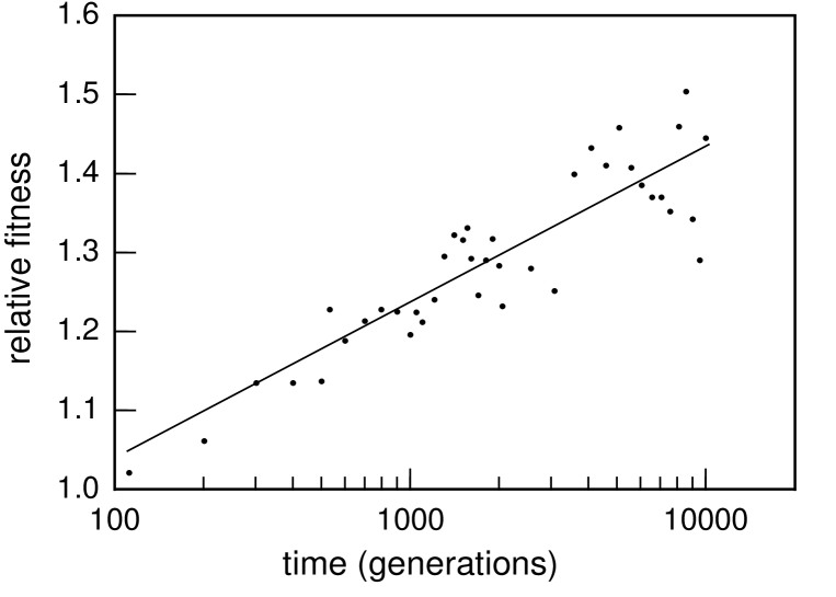
Figure 2:

The mean fitness in one population of E. Coli grown in a glucose-limited environment, is shown in a semilogarithmic plot as a function of the number of generations. The original data and a detailed description of the controlled evolution experiment can be found in Ref. [24]. Note that the data approximately follow the logarithmic fitness growth curve discussed in connection with the reset model.

3 The reset model

The ‘reset’ model includes the idea that macroevolutionary events are triggered by fitness records, and complements it with the possibility of extinctions through interspecies interactions in an ecological space. The model deals with a number of highly idealized species evolving and interacting with one other within an ‘ecology’. The whole system is conveniently depicted as a graph, in which nodes correspond to niches and edges represent interactions among the (neighbor) species which occupy them. Model species are born, evolve and eventually die. In most of the treatment below the (physical) external conditions are assumed constant. However, we additionally consider a ‘meteor’ variant of the model where the effects of changes in external conditions are modeled as random killings (i.e. unrelated to fitness ) of a fraction of the systems’ species.

The evolution part of the reset model is basically the record dynamics just described. Between evolutionary changes, no extinctions are allowed and the system remains quiescent. When a species evolves, it is assumed to modify the fitness landscape of its ecological neighbors, thus creating the possibility of extinctions. Consider a species evolving from fitness $f$ to $f^{\prime}>f$. By definition of the model update rule, those among its neighbors having fitness less than $f^{\prime}$ are declared extinct and removed from the system. In the next time step, the empty niche is ‘reset’, i.e. it becomes occupied by a freshly initialized species. This defines the reset model. Note that the reset rule depends on the rank ordering of the agents, not on the specific form of the fitness. We have implemented versions of the model with slight differences in the details of the removal and replacement of the species. However, we find the results to be robust to these changes.

In the simulations discussed below, the ecology is modeled as a regular lattice. Previously, we have investigated both one and two dimensional systems [1], obtaining very similar results, so we here confine ourselves to a 2D grid with unit lattice constant. In this grid, the neighborhood of the point $x_{0},y_{0}$ is defined as the set of integers: ${\cal N}_{0}=\{(x,y)\}$ such that $|x-x_{0}|\leq CR$ and $|y-y_{0}|\leq CR$. The only tunable model parameter is the Coupling Range, $CR$: If $CR=0$ our system reduces to a set of uncoupled agents, each searching for records in its own fitness landscape, while if $CR=\infty$ all agents are coupled to each other.

The reset dynamics could be simulated time step by time step, every time assigning for each agent a random trial fitness value, drawn from a given distribution. However, in this implementation nothing happens until the trial fitness value of a given agent exceeds the current value, a process which is computationally inefficient. Instead, we shall make use of some analytical results described below, allowing us to skip the inactive periods.

3.1 Fitness records and waiting times

Our simple choice is to draw all fitness values from a uniform distribution in the unit interval. As the first value drawn is by definition the first record $f_{1}$, this quantity is also uniformly distributed in the unit interval. The $k+1$’th record is required to exceed its predecessor and is therefore uniformly distributed in $(f_{k},1)$. The conditional probability density $p_{f}(x|k)$ that $f_{k+1}=x$ after $k$ records is given by :

$$p_{f}(x|k)=\frac{-\ln(1-x)^{k}}{k!}\;\;\;0\leq x<1.$$ (9)

The formula is trivially true for $k=0$. For $k>0$ it suffices to note that Eq. 9 solves the recursion relation $p_{f}(x|k)=\int_{0}^{x}p_{f}(x^{\prime}|k-1)(1-x^{\prime})^{-1}dx^{\prime}$, where the factor $(1-x^{\prime})^{-1}$ provides the proper normalization of a uniform density in the interval $(x^{\prime},1)$.

For later convenience we use the related fitness measure $z=-\ln(1-f)$. The probability density $g_{z}(x|k)$, that $z=x$ after $k$ records is found by a change of variables in Eq. 9 yielding

$$g_{z}(x|k)=\frac{x^{k}\exp(-x)}{k!}\;\;\;0\leq x<\infty.$$ (10)

The form of $g_{z}(x|k)$ indicates that $z|k$ arises as the sum of $k$ independent and identically distributed variables $\Delta_{1},\ldots,\Delta_{k}$, each describing the fitness increment in one evolutionary step. Their common distribution is an exponential of unit average:

$$p_{\Delta}(x)=\exp(-x)\;\;\;0\leq x<\infty.$$ (11)

It immediately follows from Eq. 10 that the average of $z$ grows linearly with the number of events and hence logarithmically in time.

Let us finally consider the distribution of the waiting times for the next record to happen given that the system has fitness $f$, with $0\leq f<1$. We assume that each trial takes one time unit. With probability $f$ an attempt does not lead to a record. The attempts being independent, the conditional probability for the waiting time to next record being $\delta$ is:

$$p_{w}(\delta|f)=f^{\delta-1}(1-f)\;\;\;\delta\in\{1,2\ldots\}$$ (12)

3.2 The reset algorithm

We are now ready to define a computationally efficient algorithm for the reset model. Although two equivalent fitness measures are in use: $f_{i}$ and $z_{i}$, with $z_{i}=-\log(1-f_{i})$ we only explicitly mention the latter in the following description.

At any fixed point of time an agent $i$ has two attributes: the fitness $z_{i}$, and the step time $t_{i}$ at which its next evolutionary step will be taken – unless the agent is killed at an earlier time by evolution in a neighbor site. Initially, the time is $t=0$ and all agents have fitness $z_{i}=0$, which means that there are no ‘living’ species in the system. The step-times $t_{i}$ for the next move are all initially set to the waiting time $\delta_{i}=1$, in accordance with Eq. 12. The core of the algorithm now iterates the following steps:

1. Move time to $t=\min_{i}\{t_{i}\}$

2. Pick the agent(s) $a_{k}$ with $t_{k}=t$, and update its (their) fitness and step-time(s):

   1. Generate the fitness change $\Delta_{k}$ according to Eq. 11

   2. Update fitness: $z_{k}\rightarrow z_{k}+\Delta_{k}$

   3. Generate the waiting time $\delta_{k}$ according to Eq. 12

   4. Update the step-time: $t_{k}\rightarrow t_{k}+\delta_{k}$

3. Select unfit neighbors and reset them:

   1. A neighbor $a_{j}$ of an updated agent $a_{k}$ is selected as unfit if $z_{j}<z_{k}$

   2. Reset fitness of unfit agents $a_{j}$: $z_{j}\rightarrow 0$

   3. Reset step-time of unfit agents: $t_{j}\rightarrow t+1$

Note that in one single pass an agent can both be updated in fitness and become tagged as unfit due to the evolution of one of its neighbors. This version of the reset rule is insensitive to the sequence in which these two events take place, which has some importance at short times, when the activity is high. Later, as evolutionary events thin out, it becomes increasingly unlikely that two neighbor sites would evolve in the same pass. Also note that the algorithm skips the increasingly long intervals of time where the system remains quiescent. This device makes it possible to run simulations spanning a large number of time decades. During the runs we collect a variety of statistics: e.g. the number of extinctions, the life-time of species, with the statistics gathered during a time window of selectable width, and the number of improvements that agents undergo during their life-time. Other statistical measures are the average fitness in the system as a function of time and the way in which empty niches are filled as the system evolves.

3.3 Analytical properties of the reset model

In a later section we present analytical results for a mean field version of the reset model. Here we like to mention a couple of properties of the full model which are easily derived: 1) punctuation in spite of the absence of stationary behavior on logarithmic time scales and 2) certainty of death for every agent.

Regarding 1) we note that the largest fitness value in the system $z_{max}$ is an increasing function of time. Indeed, when the agent ‘carrying’ this value changes its state, it either performs an evolutionary step, or it is killed by an evolving neighbor. In the former case $z_{max}$ clearly increases. In the latter, the neighbors’ new fitness value $z^{\prime}$ must exceed the previous $z_{max}$, thus becoming the new $z_{max}$. As $\overline{z}=N^{-1}\sum_{i}z_{i}>N^{-1}z_{max}$, we see that the average fitness value must increase as well. This eliminates the possibility that a system with finite $N$ will ever reach a stationary state, although it must be kept in mind that the increase will be extremely slow - i.e. logarithmic – and thus hardly perceptible at sufficiently long times.

Regarding 2), we only need consider the probability that the highest ranking agent in a system of two agents will eventually die, as the probability of being killed clearly grows with the number of neighbors. The killing must happen – if at all – for some $n\geq 1$, between the $n$’th and $n+1$’st record of the ‘victim’. Let us name these time intervals ‘epochs’. We bound from above the probability $S(n)$ that the agent survive $n$ epochs and show that $S(n)$ vanishes for $n\rightarrow\infty$. First we calculate the probability $R(n)$ that the agent be killed during its $n$’th epoch, given that it was alive at the beginning of the epoch.

Let the epoch be fixed and the fitness $f$ (or $z$) be given. Assume for the moment that the agent waits exactly $t$ steps before its next improvement. The probability that he is meanwhile overcome by his neighbor and therefore killed is

$$R(t,f,n)=\sum_{l=1}^{t}f^{l-1}(1-f)=1-f^{t}.$$ (13)

We first average over all possible values of $t$, with a weight given by Eq. 12, to obtain the probability that an agent with fitness $f$ is reset in its $n$’th epoch:

$$R(f,n)=\frac{1}{1+f}.$$ (14)

Averaging Eq. 14 over $f$ according to Eqs. 9 (and Eq. 10 after a convenient change of variable) yields the probability of being killed during epoch $n$:

$$R(n) = \int_{0}^{\infty}\frac{z^{n-1}\exp(-z)}{(n-1)!(2-\exp(-z))}dz$$ (15)

$$= \sum_{k=1}^{\infty}\frac{1}{2^{k}k^{n}}$$ (16)

The probability of being killed before the first improvement is $R(1)=\ln 2$. We also note that $R(n)>1/2$ for all $n$. Finally, the probability of surviving $n$ epochs is

$$S(n)=\Pi_{l=1}^{n}(1-R(l))<(1/2)^{n+1},$$ (17)

which vanishes in the limit $n\rightarrow\infty$ as claimed.

3.4 Simulation results

In this section we describe the behavior of the reset model obtained through numerical simulations. The data shown in this section represent a substantial numerical effort - of the order of one year of continuous calculation on a dedicated workstation. One single simulation took a full half year. Rather than reusing and modifying the Pascal code used in Ref. [1], completely new programs where developed in C by one of the authors (M. B.). This provided increased portability as well as an independent check. The current results concur with our previous simulation and extend them in several ways: The new simulations are considerably longer, revealing new features in the data and probe in addition the effect of externally imposed catastrophes (‘meteors’).

Throughout the sequel the symbols $\log$ and $\ln$ stand for base $10$ and natural logarithm respectively. We generally use $\log t$ as abscissa. As an inconvenient side effect, functions proportional to the natural logarithm of time appear in the plots as straight lines with slope $\ln 10=2.3$. All data shown stem from simulation of a system of 2500 agents located on a $50\times 50$ grid. Plotted fitness values are always the $z$ version described right above Eq. 10. An agent is defined as being active if it has fitness larger than zero.

In Fig. 3 we show, as a function of time a) the number of active agents; b) the average fitness and c) the minimum and d) the maximum fitness value among the active agents. As indicated, in each graph data are shown for $CR=0$, i.e. no coupling, $CR=2$, and $CR=4$. When $CR=0$ all agents are and remain active, except for the very first time step. The average fitness $\overline{z}$ is proportional to $\ln t$. The minimum and maximum fitness shown in plate c) and d) do the same. The punctuated behavior of the maximum fitness in the system is very clear. With $CR=2$ the number of active agents first saturates at $t\approx 10^{5}$. The average fitness goes through a cross-over at $t\approx 10^{3}$, with the slope changing from slightly above $1$ to $2.3$, which is the value for the uncoupled system. While the punctuated motion of the maximal fitness qualitatively is indistinguishable from the $CR=0$ case, it is clear that the minimal fitness stays close to zero up to $t=10^{5}$, as also expected from plate a). Similar behavior is seen for $CR=4$, except that the cross-over in average fitness appears at about $t=10^{7}$. Saturation of active agents is hardly seen, and the minimal fitness never increases.

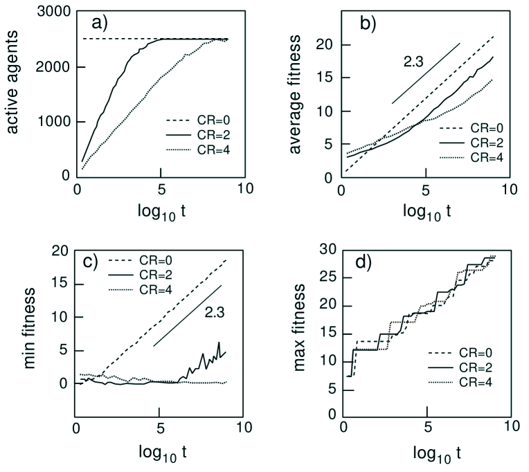
Figure 3:

As a function of time we plot: a) the number of active agents, b) the average fitness, c) the smallest fitness value among active agents and d) the largest fitness value among active agents. As indicated, in each of the subplots, different lines correspond to different degrees of coupling in the system.

In conclusion, we see that the systems’ behavior with respect to fitness eventually approaches that of an uncoupled system, with the fitness distribution moving with a velocity proportional to $\ln t$. Figure 4 describes the time dependence of the rate of extinction for a series of different coupling lengths. (In a stationary system, this quantity would remain constant) We note that coupling length $CR$ strongly affects the shape of the curves. For $CR=1$ the decay is – after a few decades – a power law with exponent $-1$. It is clear that for $CR=2$ and $3$, the data eventually reach the same asymptotic behavior. Based also on the previous results, we would guess that – independently of $CR$ – all curves reach the same asymptotic behavior. Note that, according to Eq. 7, $-1$ is the exponent characterizing the uncoupled record dynamics, if one relates extinctions and evolution by a proportionality factor. Considering the extremely large number of decades involved, it is however doubtful that the asymptotic behavior is the relevant one.

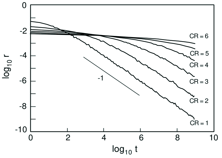
Figure 4:

The logarithm of the rate of extinction ( calculated as the fraction of extinctions taking place in each time bin ) is shown versus the natural logarithm of time for a series of different coupling lengths. For extremely long times the plots suggest that all the systems would eventually approach an algebraic decay with exponent $-1$, which corresponds to the behavior of the weakly coupled system. However, for many intermediate time scales the coupling length strongly affects the shape of the curves, with the effective decay exponent becoming progressively smaller as the coupling strength increases.

Over many decades (more than the empirical data can offer), the rate of extinction decays with an effective exponent which is numerically much smaller than $1$, and consistent with fossil data. We return to this issue in the next chapter in connection with the analysis of a continuum model [2].

Plates a) to f) in Fig. 5 each depict life span distributions in systems with $CR$ ranging from $1$ to $6$. Each plate contains nine different data sets, as most clearly seen in plate a). Each of these is the distribution of the life spans collected in a time window limited by system age $10^{0}$ – the origin of time – and $10^{i}$, with $i=1,2,3,\ldots,9$. Thus, the topmost graph is the life span distribution of all the species which died during the entire simulation. In the lowest graph only species which died during the first decade of simulation are counted. From plate d) on, i.e. for a coupling range $CR\leq 4$, all distributions are basically power-laws with an exponent of $-2$. This is again in good agreement with fossil data (Fig. 1d). At short times, a regime with a numerically lower exponent is visible, but only for small values of $CR$.

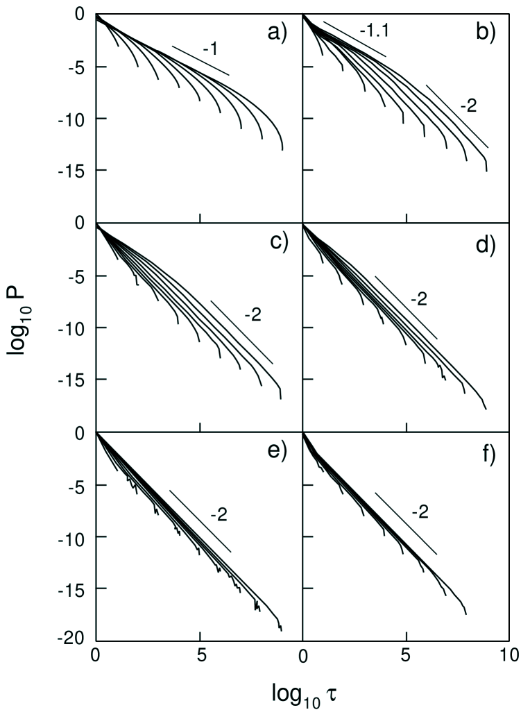
Figure 5:

This figure shows the logarithm of the life span distributions of the model species versus the logarithm of time. We investigate the effect of varying the coupling length, which increases from plate a) with $CR=1$ to plate f), with $CR=6$. In each case, we show the effect of different ways of collecting the statistics, an effect most clearly seen in plate a). In each plate we have nine different data sets: the topmost curve is the distribution of life spans collected in a time window stretching from $10^{0}$, the origin, to $10^{i}$, with $i=1,2,3\ldots 9$. Note that from plate d) on, all distributions are basically power-laws with exponent $-2$.

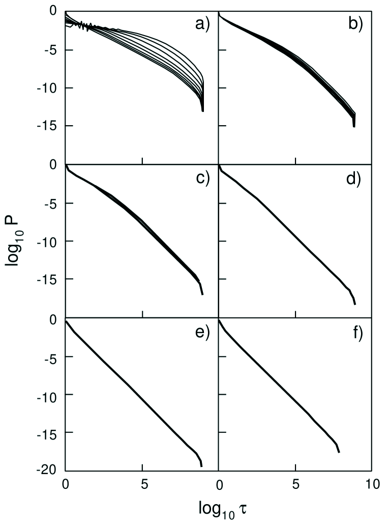
Figure 6:

This figure is similar to Fig. 5. It shows life spans distribution with the coupling length increasing from plate a), with $CR=1$ to plate f), with $CR=6$. We again have nine different data sets in each plate. Numbering them from the topmost down, the $i$’th data set is collected from time $10^{i}$ to $10^{9}$, which is the duration of the whole simulation. Again, we see that the $t^{-2}$ behavior robustly appears.

Figure 6 also depicts life-span distributions. It is organized in the same way as Fig. 5, with plates a) to f) describing $CR$ values from $1$ to $6$. The definition of the windows in system age during which the statistics is collected is however different from and complementary to that of Fig. 5. Referring for convenience to plate a), where the data sets are more easily distinguishable, the top most graph describes the life spans of agents which died between system age $10^{8}$ and $10^{9}$. The next graph pertains to those dying from $10^{7}$ to $10^{9}$ and so forth, down to the bottom one, which is identical to the top curve of the corresponding plate in Fig. 5, and which incorporates events happening during the entire run, from $10^{0}$ to $10^{9}$. Again, we see that the power law behavior with exponent $-2$ characterizes data with $CR\geq 4$. In the mean field model described below [2], the life-span distribution of a cohort – that is a set of agent born at the same time – is always a power law with exponent $-2$. Averaging over the time at which agents are born does not change this exponent, provided that the rate of extinction does not change ‘too drastically’ during the life-time of the agents. This concurs with the numerical results shown here, and further supports our explanation of the scaling form of the life span distribution obtained from the fossil record.

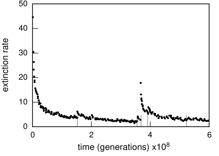
Figure 7:

We show the rate of extinction in the model as a function of time in a system subject to five external five catastrophes in which $12,14,52,12$ and $11$ % of the extanct species are killed at random (independently of their fitness) and replaced by others. The onset of the mass extinctions is marked by thin vertical line segments. Note the strong rebound effect after the mass extinctions, which is superimposed on the decaying background rate.

In order to describe the effect of external ‘catastrophes’ we simulated a modified version of the reset model, where – on top of the usual reset dynamics – a randomly chosen set of agents is destroyed and replaced at certain times $t_{1}\ldots t_{k}\ldots$. This replacement differs from the usual extinction rule in that it is indifferent to evolution, i.e. species with high and low fitness are killed with equal probability. Furthermore all the affected species are removed in a single time step, as in a mass extinction.

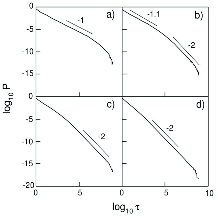
Figure 8:

We again show life-time distributions for four different coupling lengths ranging from $CR=1$ in plate a) to $CR=4$ in plate d). Even though these plots are almost indistinguishable from those of the previous two figures, the dynamics has been changed considerably by introducing five ‘external’ random catastrophes, where $12,14,52,12$ and $11$ % of the extanct species are chosen at random and removed. The corresponding times were $152.2,358.2,367.1,394.0$ and $528.4$ millions of steps. These figures show that the $t^{-2}$ behavior of the life time distribution is completely uneffected by even large external events.

We chose to introduce catastrophes roughly similar in spacing and size to the five big mass extinctions. In millions of generations the parameters $t_{1}\ldots t_{k}$ were $152.2$, $358.2$, $367.1$, $394.0$, and $528.4$. The severity of the events measured as a percent of the total extant species which were killed was $12,14,52,12$, and $11$. The massive events have a clear effect on the rate of extinction: randomizing the system makes the pace of evolution higher. Bursts of evolutionary activity after each big event are shown in Fig. 7, which depicts the rate of extinction in the relevant time window for a system with $CR=4$. The time is expressed in hundreds of millions of generation since the start of the simulation. Thin vertical line segments mark the onset of catastrophes.

The behavior of the life span distributions is shown in the four plates of Fig. 8, where the coupling range varies from a) $CR=1$ to d) $CR=4$. These curves are almost indistinguishable from their counterparts without catastrophes. The reason is simple: In the model, as well as in reality, the overwhelming majority of extinctions happens outside the big events.

4 The mean field model

Some analytical insight in the behavior of the reset model can be gained by studying a mean field version, of course at the price of introducing further simplifications. The extended model has one tunable parameter, the coupling length, which gauges the strength of interspecies interactions. If this parameter is large enough, i.e. four or above, its precise value has little influence on the behavior of the reset model. It seems therefore natural to investigate the extreme limit in which all species are coupled together. In this limit, it is possible to formulate a mean field theory as a partial differential equation for the distribution of fitness values, $P(z,t)dz$.

The material in this section mainly follows a brief account previously published in [2]. In addition we consider a model variant with a different form of the killing term. This variant has predictions in disagreement with the empirical data, but it is nevertheless included to illustrate, within this modeling context, the negative effect of choosing a symmetric type of interaction.

4.1 Generalities

The partial differential equations defining the time evolution of $P$ are designed to mimic the behavior of the reset model, where – as we have shown – a suitably defiend average fitness grows logarithmically in time. The additional fact that the distribution does not spread appreciably[27] during the course of evolution suggests that one should consider a first order transport partial differential equations (PDE).

In the simpler limiting case where no extinctions take place, we just have hill climbing in a random fitness landscape. As remarked right after Eq. 11, the average fitness then increases logarithmically in time, whence the average velocity fulfills $v=1/t=\exp(-z)$. This is generally true if each improvement is on average of the same size, a size which we for convenience assume equal to one.

With no interactions, each agent moves in fitness deterministically and independently of the others. The initial fitness distribution is therefore simply shifted in (log) time, as expressed by the following partial differential equation: $\partial P(z,t)/\partial t+\partial(v(z)P(z,t))/\partial z=0.$ We introduce interactions via a term $-gP(z,t)K(P(z,t))$, where $K$ is an effective killing rate reflecting the balance of extinction and speciation at a given $z$, while the proportionality constant $g$ determines what fraction of the system is affected by an evolutionary event. Assuming that evolution is the cause of extinction, we require that $K$ vanishes if the evolutionary current is zero. Species going extinct vacate a niche, which can be refilled at a later time. In order to formally account for this flow in and out of the system, it is convenient to introduce a ‘limbo’ state, which absorbs extinct species, and from which new species emerge at the low fitness boundary of the system. Requiring a finite upper bound to the total number of species which the physical environment can sustain amounts to a conservation law : $N(t)+\int_{0}^{\infty}P(y,t)dy=1$. In this notation $N(t)$ is the fraction of species in the limbo state, while $P(z,t)$ is the probability density of finding a living species with fitness $z$.

The above considerations result in the differential equations:

$$\frac{dN(t)}{dt}=-bN(t)+g\int_{0}^{\infty}P(y,t)K(P)dy$$ (18)

$$\frac{\partial P(z,t)}{\partial t}=-\frac{\partial(v(z)P(z,t))}{\partial z}-gP(z,t)K(P)$$ (19)

where $b$ is the rate at which species are generated at the low fitness end of the system. The initial and boundary conditions are:

$$N(t=0)=N_{0}$$ (20)

$$\forall z:P(z,t=0)=P_{0}(z)$$ (21)

$$\forall t:\int_{0}^{\infty}P(y,t)dy=1-N(t)<\infty$$ (22)

$$\forall t:P(z=0,t)=bN(t)$$ (23)

For later reference we introduce the auxiliary function

$$D(t)=\log(t+1),$$ (24)

which solves the deterministic equation of a particle moving with velocity $v(z)=\exp(-z)$: $dz/dt=\exp(-z)$, with $D(0)=0$.

A quantity often used to characterize paleontological data is the survivorship curve of a cohort or the related life span distribution[28]. In our treatment the former quantity corresponds to the probability $W_{t}(\tau)$ that an agent appearing at time $t$ will survive time $\tau$. The latter can be found from $W_{t}(\tau)$ by differentiation:

$$R_{b}(\tau\mid t)=-\frac{dW_{t}(\tau)}{d\tau}.$$ (25)

Here the subscript stands for ‘born’, to emphasize the meaning of $t$.

In our model, an agent surviving time $\tau$ has fitness $D(\tau)=\ln(\tau+1)$. Since the probability of being killed in the interval $d\tau$ is $K(P(D(\tau),t+\tau))d\tau$, $W$ fulfills the differential equation:

$$\frac{d\ln W_{t}(\tau)}{d\tau}=-gK(P(D(\tau),t+\tau));~{}\;\;\tau>0$$ (26)

with initial condition $W_{t}(\tau=0)=1$. The limit of $W$ for $\tau\rightarrow\infty$ is the probability of eventually escaping extinction. Considering that by far the largest number of species which ever lived are now extinct [29], we deem model choices leading to a non zero ultimate survival probability to be irrelevant in an evolutionary context: Interesting cases require $\int^{\infty}K(P(D(\tau),t+\tau))d\tau=\infty$.

Since, in general, the time of appearance of species is not known precisely, it is of interest to consider the effect of averaging over a time window $T$. Weighting $R_{b}(\tau\mid t)$ by the normalized rate at which new species flow into the system we obtain the average life-time distribution :

$$R(\tau)=\frac{\int_{0}^{T-\tau}N(t)R_{b}(\tau\mid t)dt}{\int_{0}^{T}N(t)dt}$$ (27)

This averaging is non trivial, if the rate at which species appear and die changes in time.

Finally, the model extinction rate is simply the number of species per unit of time which die at time $t$:

$$r(t)=g\int_{0}^{\infty}P(z,t)K(P(x,t))dx=dN/dt+bN$$ (28)

Note that in the limit $b\rightarrow\infty$, $bN(t)\rightarrow r(t)$ describes the situation considered in Ref. [1], where extinct species are immediately replaced.

4.2 Specific models

To proceed with the mathematical analysis we need to specify the killing term, which, as mentioned, should 1) only depend on the evolutionary current $v(z)P(z,t)$ and 2) vanish when $vP$ vanishes. We therefore consider two variants of the model which are consistent with these requirements:

a

The extinction rate depends on the total rate of change throughout the system: $K=(\int_{0}^{\infty}-\partial(vP)/\partial y\;dy)^{\alpha}=P(0,t)^{\alpha}$. In this case the probability of an agent being killed is independent oflifetime its fitness.

b

The extinction rate depends on the rate of change above $z$:
$K=(\int_{z}^{\infty}-\partial(vP)/\partial y\;dy)^{\alpha}=(v(z)P(z,t))^{\alpha}$. This choice similar in spirit to the model we have analyzed numerically. The assumption makes the interdependence of species asymmetrical: low-fitness species suffer if high fitness species evolve - but not vice versa. The older and fitter an agent becomes, the lesser is its probability per unit time of being killed.

In both cases the parameter $\alpha$ is introduced because it allows greater generality without unduly complicating the analysis. It is meant to describe possible correlations effects by which the size of the extinction cascade following the evolutionary step of one species becomes dependent on its fitness. If $\alpha<1$ $(>1)$, a move by an old, slowly evolving species has a larger (smaller) killing effect than one by a young, fast evolving species. In practice, good agreement with data is obtained for $\alpha$ close to but less than unity.

Model a) is at variance with empirical data. When contrasted with the good results of model b) this lack of success reveals the important role played by the asymmetry of the interactions.

4.2.1 Model a

The analysis is rather brief and mainly aimed at showing that the model is not a viable description. Utilizing $P(z=0,t)=bN(t)$, we easily find a differential equation for $N$ alone:

$$\frac{dN}{dt}=-bN+g(bN)^{\alpha}(1-N).$$ (29)

With $\tilde{N}(t)=(bN(t))^{\alpha}$ we obtain that the probability that a species born at time $t$ will survive time $\tau$ obeys:

$$\frac{d\ln W_{t}(\tau)}{d\tau}=-g\tilde{N}(\tau+t).$$ (30)

We note that Eq. 29 always has the stationary solution $N=0$. Furthermore, for $\alpha<1$ it has an additional non-zero stationary solution, $N_{s}$. A simple stability analysis shows that for $\alpha>1$ the zero solution is asymptotically approached as $\exp(-bt)$, while for $\alpha<1$ this solution is unstable and $N_{s}$ is stable. It now follows that, for $\alpha>1$, $\tilde{N}(t)$ is integrable with respect to time, leading to a non-zero ultimate survival probability. As mentioned, this behavior does not describe the extinction statistics. In the case $\alpha<1$ the right hand side of Eq. 30 is asymptotically a constant, the survival probability decays exponentially, and the rates of extinction and of birth of new species approach constants, also in disagreement with the empirical data.

Let us finally consider the case $\alpha=1$. Let $N_{0}=N(t=0)$ be the initial value of $N$, and let

$$C=\frac{N_{0}}{gN_{0}+1-g}.$$

The solution of Eq. 29 has, for $g\neq 1$, the form

$$N(t)=\frac{C(1-g)e^{-(1-g)bt}}{1-Cge^{-(1-g)bt}},$$ (31)

while for $g=1$ the solution is

$$N(t)=\frac{N_{0}}{bN_{0}t+1}.$$ (32)

We also note that, if $g>1$, then $N(t)\rightarrow\frac{g-1}{g}$ for $t\rightarrow\infty$, while if $g\leq 1$, $N(t)\rightarrow 0$ in the same limit. In both cases the decay is exponential, and both cases can be ruled out as irrelevant by the same arguments as used above.

In the case $g=1$, $N(t)$ asymptotically approaches $1/t$. Solving Eq. 30 for $W$ with $N$ given by Eq. 32 we find

$$W_{t}(\tau)=\frac{bN_{0}t+1}{bN_{0}(t+\tau)+1}.$$ (33)

The average life-time distribution is most easily obtained by averaging the conditional distribution $R_{b}(\tau\mid t)=-dW_{t}(\tau)/d\tau$ over the rate at which species appear, $bN(t)$. Omitting proportionality constants the result is

$$R(\tau)\propto\frac{1}{1+N_{0}b\tau}.$$ (34)

Even though these last choices lead to predictions which are not in strong disagreement with the data, fine tuning two parameters does not seem acceptable in the lack of specific evidence. This leads us to conclude that model a) is physically uninteresting.

4.2.2 Model b

As a first step we multiply Eq. 19 by $v(z)$, and obtain an equation for the new function $q=vP$. The solutions of this equation have the form $q(u(z,t))$, where $q$ is a function of just one variable satisfying the non-linear - but separable - ODE

$$dq/du=-gq^{\alpha+1}$$ (35)

and where $u(z,t)$ satisfies the linear inhomogeneous PDE

$$\partial u/\partial t+v(z)\partial u/\partial z=1.$$ (36)

The former equation is solved by $q=(\alpha gu)^{-1/\alpha}$. To find the solution of the latter, we let $A$ and $B$ be two arbitrary functions of a single real variable $z$, which are continuous for $z>0$ and which vanish identically for $z<0$. For $v=\exp(-z)$, the general solution has the form $u(z,t)=\epsilon\exp(z)+(1-\epsilon)t+A(t+1-\exp(z))+B(\exp(z)-(t+1))$ for some constant $\epsilon<1$. Thus, the general solution of Eq. 19 has the form

$$P(z,t)=\frac{\exp(z)}{\left[g\alpha(\exp(z)-1)+A(t+1-\exp(z))+B(\exp(z)-(t+1))\right]^{1/\alpha}}.$$ (37)

Utilizing the initial and boundary conditions, we find

$$A(z)=(bN(z))^{-\alpha},\;\;z>0$$ (38)

and

$$B(z)=(z+1)^{\alpha}P_{0}(\log(z+1))^{-\alpha}-g\alpha z,\;\;z>0.$$ (39)

Equation 37 can now be reshuffled into

$$P(z,t)=\frac{\exp(z)}{\left[g\alpha t+(\exp(z)-t)^{\alpha}P_{0}^{-\alpha}(\log(\exp(z)-t))\right]^{1/\alpha}};~{}\;\;z>D(t)$$ (40)

$$P(z,t)=\frac{\exp(z)}{\left[g\alpha(\exp(z)-1)+(bN(t+1-\exp(z)))^{-\alpha}\right]^{1/\alpha}};~{}\;\;z<D(t)$$ (41)

Note that the solution is continuous in $z$, although its derivative will in general be discontinuous at $z=D(t)$.

The survival probability of a species born at time $t$, obtained by solving Eq. 26, is

$$W_{t}(\tau)=\left[\frac{(bN(t))^{-\alpha}}{(bN(t))^{-\alpha}+g\alpha\tau}\right]^{1/\alpha}.$$ (42)

As $W$ vanishes for large $\tau$ all species eventually go extinct. This happens here for all values of $\alpha$, unlike the case previously described, where ultimate extinction with probability one is only achieved for $\alpha<1$. The above formula expresses a survivorship curve of a cohort[28], and the corresponding distribution of life spans follows from it by differentiation with respect of time (see Eq. 25). If $\alpha$ is close to unity, we find a $\tau^{-1}$ law for the former quantity, and a $\tau^{-2}$ for the latter, which is in good agreement with paleontological evidence. Further analysis of the model explains what happens when life span distributions are averaged over time dependent rates of extinctions and speciation.

For the sake of simplicity we only consider a limit case in which all probability is initially in the limbo state. This situation can e.g. be achieved by a limiting procedure, where 1) we choose $P_{0}(z)=bC/(b+C)\exp(-zC)$ and $N(t=0)=C/(C+b)$ for some $C$ (this fulfills the boundary conditions for any finite $C$), and 2) we subsequently let $C\rightarrow\infty$. In this limit the expression for $P(z,t)$ in the region $z<D(t)$ remains Eq. 41, while $P$ vanishes identically for $z>D(t)$.

A non-linear integral equation containing $N(t)$ alone is obtained by integration of Eq. 41, followed by a change of variables. The result is

$$1-N(t)=\int_{0}^{t}\frac{dy}{\left[g\alpha(t-y)+(bN(y))^{-\alpha}\right]^{1/\alpha}}.\\$$ (43)

Differentiating Eq. 43 with respect to time, and utilizing Eq. 28, we find the extinction rate:

$$r(t)=\int_{0}^{t}\frac{g\;dy}{\left[g\alpha(t-y)+(bN(y))^{-\alpha}\right]^{1+1/\alpha}}.\\$$ (44)

The life time distribution averaged over a window $T$ is found by using Eq. 41 in conjunction with Eqs. 26 and 27. This yields

$$R(\tau)=\frac{\int_{\tau}^{T}\frac{gdy}{\left[g\alpha\tau+(bN(y))^{-\alpha}\right]^{1+1/\alpha}}}{\int_{\tau}^{T}r(y)dy}.$$ (45)

Equivalently, one can average the life-time distribution of species born at time $t$ over the normalized rate at which new species flow into the system. This yields

$$R(\tau)=\frac{\int_{0}^{T-\tau}\frac{gdy}{\left[g\alpha\tau+(bN(y))^{-\alpha}\right]^{1+1/\alpha}}}{\int_{0}^{T-\tau}bN(y)dy}.$$ (46)

Finally, in order to better describe the $\tau$ dependence of $R$, it is useful to express $N^{-\alpha}$ in terms of the survival probability using Eq. 42. The procedure yields:

$$R(\tau)=g(g\alpha\tau)^{-1-1/\alpha}\frac{\int_{\tau}^{T}(1-W_{y}^{\alpha}(\tau))^{1+1/\alpha}dy}{\int_{\tau}^{T}r(y)dy}.$$ (47)

The $\tau$ dependence stemming from the limits of the above integrals is only relevant when $\tau\approx T$, and can be safely ignored, if $T$ is sufficiently large. Furthermore, Eq.  42 shows that, if $\alpha g\tau>(bN(y))^{-\alpha}$ is fulfilled throughout the integration interval, then $W_{y}(\tau)\approx 0$, and the $\tau$ dependence of the integrand becomes negligible. In this case, $R\propto\tau^{-1-1/\alpha}$, i.e. an algebraic decay with an exponent close to $-2$ for $\alpha\approx 1$. As shown numerically below, the assumption regarding $r(t)$ is confirmed by model calculations for a wide range of parameter values. In particular, when $\alpha$ close to unity the model yields $r(t)\approx bN(t)\approx t^{-\delta}$ , with $\delta$ close to $0.5$ for a considerable time range. In this situation, even though $\tau<<T$, $\tau>T^{\delta\alpha}$ can be fulfilled for reasonable $\tau$ values. Consider for instance $\delta=0.5$, $\alpha=1$ and $T=10^{12}$ (generations). The power law behavior with exponent $-2$ then occurs for $\tau>3\times 10^{4}$ (generations) which is rather short life-time. The cross-over from a slow decay to the $\tau^{-2}$ law is also found in simulations of the full model, where moves to shorter times as the degree of interaction among species increases, and the decay exponent $\delta$ correspondingly decreases. (see e.g. Figs. 5 and 6).

From the point of view of biological data assuming that the extinction rate varies slowly over some typical time scale of species life time, seems very reasonable: The rate of extinction appears to change appreciably on a scale of a hundred million years, while the range of species life-times is better expressed in millions of years.

Returning to the analysis of the model, we first note a major difference in the asymptotic behavior for $\alpha<1$ and $\alpha\geq 1$. In both cases the time independent function $P_{\infty}(z)$ obtained by taking $t\rightarrow\infty$ and by setting $N(t)=N_{\infty}\neq 0$ in Eq. 41 formally satisfies the model equations. However, only for $\alpha<1$ is $P_{\infty}(z)$ normalizable and thus a true solution. The corresponding steady state value of $N$, $N_{\infty}$ is then implicitly given by the relation $1-N_{\infty}=(bN_{\infty})^{1-\alpha}/(g(1-\alpha))$, which always has a solution in the unit interval.

In the case $\alpha\geq 1$, normalizability of $P(z,t)$ requires that $N(t)\rightarrow 0$ for $t\rightarrow\infty$. No steady state solution can then exists, since $P(z,t)$ vanishes with $t$ at any fixed $z$, as e.g. in the familiar case of simple diffusion on the infinite line.

Even when a steady state solution exists the fact that $D(t)$ only changes logarithmically shows, in connection with Eqs. 40 and 41, that the relaxation is extremely slow, and that, depending on the initial condition, the transient behavior might well be the only relevant one.

The long time asymptotic solution can be obtained explicitly in the case $\alpha=1$. If $bt>>1$ the term $dN/dt$ in Eq. 18 is negligible, and $bN(t)\approx r(t)$. In this limit we can also neglect $N$ compared to one, thus finding the following approximate equation for the rate of extinction:

$$1=\int_{0}^{t}\frac{gdy}{g(t-y)+r(y)^{-1}},$$ (48)

which is solved by $r(t)=(gt)^{-1}$.

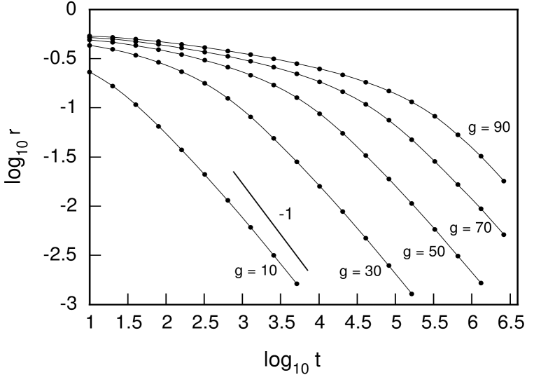
Figure 9:

We show the logarithm of rate of extinction of the analytical model plotted as a function of the logarithm of time, for $\alpha=1$, $b=1$ and various values of the coupling constant $g$. Note the change from a slow to a faster decay, and the fact that the cross-over time between the two regimes increases with $g$. This behavior strongly resembles that of the full reset model shown in Fig. 4.

In Fig. 9 we show the the rate of extinction of the mean field model as a function of time, for $\alpha=1$, $b=1$ and several choices of the coupling constant $g$. Note the striking similarity with the extinction rate of the full reset model, shown in Fig. 4. In both cases there is a cross-over from a power-law with a (numerically) small effective decay exponent to to another power-law with exponent approaching $-1$. Furthermore, the cross-over time strongly increases with the degree of coupling, which is expressed in one case by thethe parameter $CR$ and in the other by $g$.

5 Summary and conclusion

In this paper we have described a model of evolutionary dynamics which builds on two basic elements: 1) the dynamics of a single species in a constant physical environment is assumed to follow a record statistics, leading to a logarithmic improvement of different evolutionary measures, and 2) extinctions are caused by co-evolution: the evolution of a species removes its less fit neighbors. This approach is analyzed numerically as well as analytically in a simpler, mean field version.

Our first model assumption stems from considering the behavior of random walks in highly dimensional rugged fitness landscapes. It stresses the fact that a species maintains a record of its past history through a stable genetic pool and states that the statistical properties of this pool can only change when a random mutation appears, which is better than the ‘best so far’. Its predictions are in good agreement with the intersting empirical data obtained by Lenski and Travisano [24] on the evolution of bacterial cultures in a nutrient deprived environment. Our second assumption leads to good agreement with empirical data regarding the life time distribution of species and the decay of the extinction rate. The size distribution of events, which is the main focus of many other (stationary) approaches, is in our case derived from the the rate of extinction, as discussed already in the introduction. Also in this respect our model is in good agreement with the data. The behavior of the system as a whole is characterized by the fact that, as time goes, the dynamics approaches that of a single agent optimizing its fitness. In this sense one could talk about increasing correlations among the species. When the system is partly randomized by external catastrophes modeling sudden changes of the environment, the whole system is set back in its evolution as shown by the strong rebound effect in the rate of extinction. Interestingly, catastrophes do not change the life-time distribution in any significant way. In summary, our model offers a single, albeit approximate, explanation of most evolutionary data, linking the distribution of life spans with the behavior of the rate of extinction and of the distribution of event sizes.

From the vantage point of a theoretical physicist, the scale invariance present in evolution and extinction data begs for an explanation. As mentioned in our introductory discussion several different theoretical approaches currently exist. On the opposite extreme of the modeling spectrum, purely statistical considerations have lead to the suggestion that extinctions are basically due to external periodic forcing, stemming impacts from from celestial bodies[18, 19]. As biological evolution is a non-reproducible experiment (within the time scales available to human observers ), the dilemma of what really has happened might not be easily solved. Biological history contains a good measure of frozen accidents which do not have and probably do not require specific explanations. Therefore, it seems hard (and pointless) to exclude that different mechanisms for evolution and extinction (i.e. rocks from the sky and species competition) could have play together to shape the course of evolution. We would expect progress in clarifying the relative importance of various modeling elements to come from closer scrutiny of the basic assumptions, particularly at the level of population dynamics.

Acknowledgments
P. S. would like to thank the Santa Fe Institute of Complex Studies for nice hospitality and Mark Newman for interesting discussions. This work was supported in part by Statens Naturvidenskabelige Forskningsråd.

References

- [1] Paolo Sibani, Michel R. Schmidt and Preben Alstrøm Phys. Rev. Lett., 75, 2055 (1995)
- [2] Paolo Sibani Phys. Rev. Lett., 79, 1413 (1997)
- [3] J. John Sepkowski, Jr. Paleobiology, 19, 43 (1993)
- [4] David M. Raup, The role of extinction in evolution, in Tempo and mode in evolution, Walter M. Fitch and Francisco J. Ayala Ed., National Academy of Sciences, 1995.
- [5] D. M. Raup Extinction: Bad genes or bad luck? (Norton, New York, 1991)
- [6] David M. Raup and J. John Sepkoski Science, 215, 1501 (1982)
- [7] James W. Valentine, Late Precambrian Bilaterians: Grades and Clades in Tempo and mode in evolution, Walter M. Fitch and Francisco J. Ayala Ed., National Academy of Sciences, 1995.
- [8] We note that in more recent works Raup criticizes the separation in ‘background’ and ‘mass’ extinctions as artificial. See e.g. Ref. [4]. Our data analysis (i.e. the values of the exponents) depends very weakly on making this assumption. However, at least within the theoretical model we propose, the distinction between ‘mass’ and ‘background’ is meaningful and corresponds to two different modes of extinction, one endogenous and the other exogenous. Our model predicts the decaying background extinctions and robustly absorbes externally imposed mass extinctions.
- [9] Luis W. Alvarez, Walter Alvarez, Frank Asaro and Helen V. Michel Science 208, 1095 (1980)
- [10] David M. Raup Paleobiology, 17, 37 (1991)
- [11] P. Bak and K. Sneppen Phys. Rev. Lett., 71, 4083 (1993)
- [12] Kim Sneppen, Per Bak, Henrik Flyvbjerg and Mogens H. Jensen. Proc. Natl. Acad. Sci. USA, 92, 5209 (1995)
- [13] M. E. J. Newman and B. W. Roberts Proc. R. Soc. Lond. B , 260, 31, (1995)
- [14] M. E. J. Newman J. Theor. Biol. , in press
- [15] Kim Sneppen and M. E. J. Newman Physica D, in press
- [16] Ricard V. Solé, Jordi Bascompte and Susanna C. Manrubia Proc. Roy. Soc. B, 263, 1407 (1996)
- [17] S. C. Manrubia and M. Paczuski preprint cond-mat/9607066
- [18] David M. Raup and J. John Sepkoski, Jr. Proc. Natl. Acad. Sci. USA, 81, 801 (1984)
- [19] J. John Sepkoski, Jr. Journal of the Geological Society, 146, 7 (1989)
- [20] S. Wright Evolution, 36, 427 (1995)
- [21] G. Weisbuch, in Spin glasses and biology, edited by D. L. Stein (world Scientific, Singapore, 1992), pp. 141–158.
- [22] M. Kimura. The neutral theory of molecular evolution Cambridge University Press 1983.
- [23] Stuart Kauffman At home in the universe, Chapt. 9, Oxford University Press (1995)
- [24] Richard E. Lenski and Michael Travisano Proc. Natl. Acad. Sci. USA, 91, 6808 (1994), and Dynamics of adaptation and diversification, in Tempo and mode in evolution, Walter M. Fitch and Francisco J. Ayala Ed., National Academy of Sciences (1995)
- [25] Paolo Sibani and Peter B. Littlewood Phys. Rev. Lett., 71, 1485 (1993)
- [26] Walter Rudin Real and complex analysis, McGraw-Hill (1966)
- [27] M. Schmidt Master Thesis, Odense Universitet, (1995)
- [28] David M. Raup Paleobiology, 4, 42 (1978)
- [29] David M. Raup Science, 231, 1528(1986)