Domain formation in transitions with noise and time-dependent bifurcation parameter

Many physical systems undergo a transition from a spatially uniform state to one of lower symmetry. Classical examples are the formation of magnetic domains and the Rayleigh-Benard instability [1]. Such systems are commonly modeled by a simple differential equation, having a bifurcation parameter with a critical value at which the spatially uniform state loses stability. Noise is often assumed to provide the initial symmetry-breaking perturbation permitting the system to choose one of the available lower-symmetry states, but is not often explicitly included in mathematical models. However, when the bifurcation parameter is slowly increased through its critical value it is necessary to consider noise explicitly.

The phenomenon of delayed bifurcation and its sensitivity to noise has been reported in the case of non-autonomous stochastic ordinary differential equations [2]; here the corresponding phenomenon is examined in partial differential equations. A characteristic length for the spatial pattern is demonstrated from a stochastic partial differential equation (SPDE), supported by numerical simulations. Noise is added in such a way that it has no correlation length of its own (white in space and time) and a finite difference algorithm is used whose continuum limit is an SPDE.

The mathematical description of transitions is in terms of a space-dependent order parameter $Y$ and a bifurcation parameter $g$. Because it is the simplest model with the essential features, the real Ginzburg–Landau equation (GL) is considered first. Results are also presented for the Swift–Hohenberg equation (SH), that is more explicitly designed to model Rayleigh-Benard convection.

When the bifurcation parameter $g$ is constant the following is found. For $g<0$, in both GL and SH, the solution with $Y$ everywhere $0$ is stable. In GL for $g>0$ one sees a pattern of regions where $Y$ is positive and regions where $Y$ is negative (domains) separated by narrow transition layers. In SH for $g>0$ there is a structure resembling a pattern of parallel rolls, interrupted by defects.

When $g$ is slowly increased through $0$ in the presence of noise a characteristic length is produced as follows. The field $Y$ remains everywhere small until well after $g$ passes through $0$. At $g\simeq g_{c}$, where

$$g_{c}=\sqrt{2\mu|\ln\epsilon|},$$ (1)

$\mu$ is the rate of increase of $g$ and $\epsilon$ is the amplitude of the noise, $Y$ at last becomes ${\cal O}{(1)}$ and the spatial pattern present is frozen in by the nonlinearity. Thereafter one observes spatial structure with characteristic size proportional to $({|\ln\epsilon|/\mu})^{{1\over 4}}$. In GL this length is the typical size of the domains; in SH it is the typical distance betwen defects.

The results reported here were obtained by solving SPDEs [3] of the following dimensionless form for stochastic processes $Y$ depending on $x$ and $t$:

$${\rm d}Y=[g(t)Y-Y^{3}+{\cal L}Y]{\rm d}t+\epsilon{\rm d}W.$$ (2)

The equations were solved as initial value problems, with $g(t)=\mu t$ slowly increased from $-1$ to $1$. Here $Y:[0,L]^{m}\times[-{1\over\mu},{1\over\mu}]\times\Omega\to\cal{R}$, $\Omega$ is a probability space and $W$ is the Brownian sheet [4], the generalisation of the Wiener process (standard Brownian motion) to processes dependent on both space and time. Periodic boundaries in $x$ are used so that any spatial structure is not a boundary effect. The constants $\mu$, $\epsilon$ and ${1\over L}$ are all $\ll 1$. Results are reported for ${\cal L}=\Delta$ (GL) and ${\cal L}=-(1+\Delta)^{2}$ (SH) where $\Delta=\sum_{i=1}^{m}{\partial^{2}\over\partial x_{i}^{2}}$, the Laplacian in ${\cal R}^{m}$.

In the first order finite difference algorithm for numerical realisations of the lattice version of (2), $y_{t+\Delta t}(i)$ is generated from $y_{t}(i)$ as follows:

$$y_{t+\Delta t}(i)= y_{t}(i)+[\mu ty_{t}(i)-y_{t}^{3}(i)+\tilde{\cal{L}}y_{t}(i)]\Delta t$$ (3)

$$+\epsilon\,\left(\Delta x\right)^{-{m\over 2}}\,n_{t}(i)\,\sqrt{\Delta t}.$$ (4)

In (3), $y_{t}(i)$ is numerical approximation to the value of $Y$ at site $i$ at time $t$ and $\tilde{\cal{L}}$ is the discrete version of ${\cal{L}}$. The $n_{t}(i)$ are Gaussian random variables with unit variance, independent of each other, of the values at other sites, and of the values at other times.

It is also possible to introduce multiplicative noise, for example to make $g$ a random function of space and time [5,6]. The effect in that case is proportional to the magnitude of the noise and is thus less dramatic at small intensities than that of additive noise.

The timing of the emergence of spatial structure can be understood by deriving the stochastic ordinary differential equation for the most unstable Fourier mode, which is of the form [7]

$${\rm d}y=[g(t)y-y^{3}]{\rm d}t+\epsilon{\rm d}w,$$ (5)

where $w$ is the Wiener process. Trajectories of (4) remain close to $y=0$ until well after $g=0$, then jump abruptly towards one of the new attractors (Figure 1). The value of $g$ at the jump can be determined by solving the linearised version ; for $\mu\ll 1$ it is a random variable with mean approximately $g_{c}$ and standard deviation proportional to $\mu$ [8].

FIG. 1.: Dynamic pitchfork bifurcation with noise. The dotted lines are the loci of stable fixed points of $\dot{y}=gy-y^{3}$ as a function of $g$. The solid lines are solutions of the non-autonomous SDE (4) with $g=\mu t$, for noise levels $\epsilon=10^{-3}$, $10^{-6}$, $10^{-9}$, $10^{-12}$. (In each case $\mu=0.01$ and the initial condition is $y=1.0$ at $g=-1.0$.)

The Ginzburg-Landau equation is a simple model of a spatially extended system where a uniform state loses stability to a collection of non-symmetric states. When $g$ is fixed and positive in this equation, a pattern of domains is found. In each domain, $Y$ is close either to $\sqrt{g}$ or to $-\sqrt{g}$. The gradual merging of domains on extremely long timescales [9] is not the subject of this paper; here the focus is on how the domains are formed by a slow increase of the bifurcation parameter through $0$. An example is depicted in Figure 2: a pattern of domains emerges when $Y$ is everywhere small and is frozen in at $g\simeq g_{c}$. When $Y$ is small an excellent approximation to the correlation function, $c(x)=\big{<}Y_{t}(v)Y_{t}(x+v)\big{>}$, can be calculated from the solution of the linearised version of (2) (that is, without the cubic term). The correlation length at $g=g_{c}$ becomes the characteristic length for spatial structure after $g=g_{c}$.

For GL, the solution of the linearised version of (2) is:

$$Y_{t}(x)=\int_{[0,L]^{m}}G({\scriptstyle t,-{1\over\mu},x,v})f(v){\rm d}v+$$ (6)

$$\epsilon\int_{-{1\over\mu}}^{t}\int_{[0,L]^{m}}G({\scriptstyle t,s,x,v}){\rm d}v{\rm d}W_{s}(v),$$ (7)

FIG. 2.: Dynamic transition, GL, one space dimension. Four configurations, $Y_{t}(x)$, are shown from one numerically-generated realisation of the SPDE (note the different vertical scales). Nonlinear terms become important when $g\simeq 0.64$; their effect is to freeze in the spatial structure. ($L=300$, $\mu=0.01$, $\epsilon=10^{-10}$.)

where $G({\scriptstyle t,s,x,v})=$

$${\scriptstyle[4\pi(t-s)]}^{-{m\over 2}}\exp\left({\scriptstyle-{\,\,(x-v)^{2}\over 4(t-s)}-\mu(t^{2}-s^{2})}\right)$$

with $x-v$ understood modulo $[0,L]^{m}$. The first term, dependent on the initial data $f(x)$, relaxes quickly to very small values and remains negligible if $2\mu|\ln\epsilon|<1$. The correlation function is therefore obtained from the second integral in (5). The mean of the product of two such stochastic integrals is an ordinary integral [4]. Performing the integration over space [7], assuming that $L>({8\over\mu})^{{1\over 2}}$, gives

$$c(x)=\epsilon^{2}\int_{0}^{t}{{\rm e}^{\mu(t^{2}-s^{2})}{\rm e}^{{-x^{2}\over 8(t-s)}}\over[8\pi(t-s)]^{{m\over 2}}}{\rm d}s.$$ (8)

Before $g$ approaches $0$, the correlation function differs by only ${\cal{O}}({\mu\over g^{2}})$ from its static ($g=$constant) form [7]; it remains well-behaved as $g$ passes through $0$ and, for $g>\sqrt{\mu}$, is well approximated by:

$$c(x)\simeq{\epsilon^{2}{\rm e}^{\mu t^{2}}\over({8\mu t})^{{m\over 2}}}{\rm e}^{-{x^{2}\over 8t}}.$$ (9)

For ${1\over\sqrt{\mu}}<g<g_{c}$, typical values of $Y(x)$ increase exponentially fast and the correlation length is proportional to $\sqrt{t}$. Effectively noise acts for $g\leq\sqrt{\mu}$ to provide an initial condition for the subsequent evolution. At a value of $g$ that is a random variable with mean $g\simeq g_{c}$ and standard deviation proportional to $\mu$, the cubic nonlinearity becomes important. Its effect is to freeze in the spatial structure; no perceptible changes occur between $g=g_{c}$ and $g=1$.

In one space dimension it is possible to put the scenario just described to quantitative test by producing numerous realisations like that of Fig.2 and recording the number of times $Y$ crosses upwards through $0$ in the domain $[0,L]$ at $g=1$. In Fig.3 the average number of upcrossings is displayed as a function of the sweep rate $\mu$. The solid line is the expected number of upcrossings of zero,

$$r={L\over 2\pi}\left({-c^{\prime\prime}(0)\over c(0)}\right)^{\frac{1}{2}}={L\over 4\pi}\left({\mu\over 2|\ln\epsilon|}\right)^{{1\over 4}},$$ (10)

for a field with correlation function (7) at $g=g_{c}$ [10]. The hypothesis that the spatial pattern does not change after $g=g_{c}$ is succesful.

FIG. 3.: Number of zero crossings after a dynamic transition. The dots are the mean number of upcrossings of $0$ at $g=1$ in numerical realisations of GL in one space dimension. The solid line is the prediction based on the assumption that the correlation function (7) is valid until $g=g_{c}$, after which time the spatial pattern does not change. ($\epsilon=10^{-4}$ and $L=800$.)

In one space dimension, the solution of the SPDE (2) is a stochastic process with values in a space of continuous functions [3,12,13]. That is, for fixed $\omega\in\Omega$ and $t\in[-{1\over\mu},{1\over\mu}]$, one obtains a configuration, $Y_{t}(x)$, that is a continuous function of $x$. This can be pictured as the shape of a string at time $t$ that is constantly subject to small random impulses all along its length. In more than one space dimension, however, the $Y_{t}(x)$ are not necessarily continuous functions but only distributions [3,12]. Typically the correlation function $c(x)$ diverges at $x=0$. In the dynamic equations studied here, however, the divergent part does not grow exponentially for $g>0$, and by $g=g_{c}$ it is only apparent on extremely small scales, beyond the resolution of any feasible finite difference algorithm. Figure 4 depicts configurations at $g=1$ from realisations of (2) in two space dimensions. In Figures 4(a) and 4(b) (GL) one sees that a faster rate of increase of $g$ results in a smaller average domain size. The SPDEs were simulated on a grid of $512\times 512$ points with second order timestepping [13].

   

   

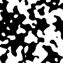
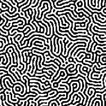
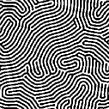
FIG. 4.: Two-dimensional pattern at $g=1$: smaller $\mu$ means larger characteristic length. In black regions $Y<0$; in white or grey regions $Y>0$. In GL, (a) and (b), the typical domain size decreases with $\mu$ , the rate of increase of $g$. In SH, (c) and (d), where there is a short-range structure resembling parallel rolls, the effect of reducing $\mu$ is to reduce the number of defects. 4(a): GL, $L=300$, $\epsilon=10^{-5}$, $\mu=0.03$. 4(b): GL, $L=300$, $\epsilon=10^{-5}$, $\mu=0.003$. 4(c): SH, $L=200$, $\epsilon=10^{-5}$, $\mu=0.01$. 4(d): SH, $L=200$, $\epsilon=10^{-5}$, $\mu=0.001$.

The essential difference between the Swift-Hohenberg and Ginzburg–Landau models is that the first spatial Fourier mode to become unstable has $k=1$ rather than

$k=0$. Hence there is a preferred small-scale pattern that resembles the parallel rolls seen in experiments. However, there is no preferred orientation of the roll pattern and when the correlation length is smaller than the system size, many defects are found, separating regions where the rolls have different orientations. When $g$ is increased through $0$, the number of defects resulting decreases when $\mu$ decreases – Fig.4(c) and (d). Here a grid of $300\times 300$ points was used with first order timestepping.

A notable feature of dynamic bifurcations and dynamic transitions is that the evolution for $g>0$ is independent of the initial conditions (provided they are such that that the system descends into the noise). Noise acts, near $g=0$,

to wipe out the memory of the system and to provide an initial condition for the subsequent evolution. The correlation function (7) is, for example, a natural initial condition for studying the dynamics of defects and phase separation because it emerges from a slow increase to supercritical of the bifurcation parameter in the presence of space-time noise, mimicking an idealised experimental situation.

In summary, dynamic transitions are analysed in models of spatially extended systems with white noise. The correlation length that emerges from the noise during a slow sweep past $g=0$ is frozen in by the nonlinearity as a characteristic length proportional to $({|\ln\epsilon|/\mu})^{{1\over 4}}$ where $\mu$ is the rate of increase of the bifurcation parameter and $\epsilon$ is the amplitude of the noise.