Modeling diffusion of innovations with probabilistic cellular automata

Abstract: We present a family of one-dimensional cellular automata modeling the diffusion of an innovation in a population. Starting from simple deterministic rules, we construct models parameterized by the interaction range and exhibiting a second-order phase transition. We show that the number of individuals who eventually keep adopting the innovation strongly depends on connectivity between individuals.

1 Introduction

Diffusion phenomena in social systems such as spread of news, rumors or innovations have been extensively studied for the past three decades by social scientists, geographers, economists, as well as management and marketing scholars. Traditionally, ordinary differential equations have been used to model these phenomena, beginning with the Bass model (Bass, 1969) and ending with sophisticated models that take into account learning, risk aversion, nature of innovation, etc. (Mahajan et al., 1990; Mahajan and Peterson, 1985; Rogers, 1995). Models incorporating space and spatial distribution of individuals have been also proposed, although most research in this field has been directed to refining of the discrete Hägerstrand models (Hägerstrand, 1952, 1965) and to constructing partial differential equations similar to diffusion equations known to physicists (Haynes et al., 1977).

Diffusion of innovations (we will use this term in a general sense, meaning also news, rumors, new products, etc.) is usually defined as a process by which the innovation “is communicated through certain channels over time among the members of a social system” (Rogers, 1995). In most cases, these communication channels have a rather short range, i.e. in our decisions we are heavily influenced by our friends, family, coworkers, but not that much by unknown people in distant cities. This local nature of social interactions makes cellular automata (CA) a well-adapted tool in modeling diffusion phenomena. In fact, epidemic models formulated in terms of automata networks have been successfully constructed in recent years (Boccara and Cheong, 1992, 1993; Boccara et al., 1994).

2 Simple deterministic models

We will construct models of diffusion of innovations based on elementary (radius-1) cellular automata (Wolfram, 1986). If $s(i,t)$ denotes the state of lattice site $i$ at time $t$, the function $(i,t)\mapsto s(i,t)$ is a mapping from ${\mathbf{Z}}\times{\mathbf{N}}$ to ${\mathbf{Z}}_{2}=\{0,1\}$. Given a function $f:\{0,1\}^{2r+1}\mapsto\{0,1\}$, the discrete dynamical system

$$s(i,t+1)=f(s(i-r,t),s(i-r+1,t),\ldots,s(i+r,t))$$ (1)

is called a cellular automaton (CA) of radius $r$, and $f$ is called its local (function) rule.

In the simplest version of our model, the sites of an infinite lattice are all occupied by individuals. The individuals are of two different types: adopters $\Big{(}s(i,t)=1\Big{)}$ and neutrals $\Big{(}s(i,t)=0\Big{)}$. Moreover, we wil assume that an individual can get information only from it two nearest neighbors. To simplify our model, we will also assume that once an individual becomes an adopter, he remains an adopter, i.e. his state cannot change. This condition fixes four entries in the rule table: $\left\{0,1,0\right\}\rightarrow 1$, $\left\{0,1,1\right\}\rightarrow 1$, $\left\{1,1,0\right\}\rightarrow 1$ and $\left\{1,1,1\right\}\rightarrow 1$, and since the information comes from nearest neighbors, if both are neutral, then the individual will stay neutral, i.e., $\left\{0,0,0\right\}\rightarrow 0$. This leaves three entries in the rule table to be determined, and this can be done in $2^{3}=8$ ways, as shown in Table 1. The first

code	1,1,1	1,1,0	1,0,1	1,0,0	0,1,1	0,1,0	0,0,1	0,0,0
204	1	1	0	0	1	1	0	0
206	1	1	0	0	1	1	1	0
220	1	1	0	1	1	1	0	0
222	1	1	0	1	1	1	1	0
236	1	1	1	0	1	1	0	0
238	1	1	1	0	1	1	1	0
252	1	1	1	1	1	1	0	0
254	1	1	1	1	1	1	1	0

Table 1: Eight possible elementary rules for diffusion of an innovation.

Rule $204$ (for rule codes cf. Wolfram 86) listed in this table is just the identity, and it will be excluded from further considerations. Rules $220$ and $252$ can be obtained respectively from $206$ and $238$ by spatial reflection, therefore they will be excluded too. This leaves us with five distinct rules.

Rule 254:

An individual adopts if, at least, one of his neighbors is an adopter.

Rule 238:

An individual adopts only if his right neighbor is an adopter.

Rule 222:

An individual adopts only if exactly one of his neighbors is an adopter.

Rule 206:

An individual adopts only if his right neighbor is an adopter and its left neighbor is neutral.

Rule 236:

An individual adopts only if both his neighbors are adopters.

We will now demonstrate that in all five cases, the density of adopters $\rho(t)$ at time $t$ can be exactly computed, assuming that we start from a disordered initial configuration with $\rho(0)=\rho_{0}$.

(i) In order to understand the dynamics of Rule 254, we can view the initial configuration as clusters of ones separated by clusters of zeros. Only neutral sites adjacent to a cluster of ones change their state, while all other neutral sites remain neutral, as shown in the example below (sites that will change their state to $1$ in the next time step are underlined):

$\cdots$ 1 0 0 0 1 1 0 0 0 0 1 1 $\cdots$

This implies that the length $l$ of every cluster of zeros decreases by two every time step, i.e.

$$M(l,t+1)=M(l+2,t),$$ (2)

where $M(l,t)$ denotes a number of clusters of zeros of size $s$ per site at time $t$, and therefore

$$M(l,t)=M(l+2t,0).$$ (3)

For a random initial configuration with initial density $\rho_{0}$, the cluster density is given by $M(l,0)=(1-\rho_{0})^{l}\rho_{0}^{2}$, hence

$$M(l,t)=(1-\rho_{0})^{l+2t}\rho_{0}^{2}.$$ (4)

The density of zeros at time $t$, denoted by $\eta(t)$, is given by

$$\eta(t)=\sum_{l=1}^{\infty}lM(l,t)=(1-\rho_{0})^{2t+1},$$ (5)

and finally the density of ones $\rho(t)$ is equal to

$$\rho(t)=1-\eta(t)=1-(1-\rho_{0})^{2t+1}.$$ (6)

(ii) For Rule $238$, the derivation is similar, except that now every cluster of zeros decreases by one every time step, which means that we have to replace $2t$ by $t$ in the previous result, i.e.

$$\rho(t)=1-(1-\rho_{0})^{t+1}.$$ (7)

(iii) In Rule 222, individuals “dislike overcrowding”, and they do not become adopters if their two neighbors are already adopters. adopt if both neighbors adopted, i.e. $\left\{1,0,1\right\}\rightarrow 0$. As a consequence, clusters of size $l>1$ decrease their size by two units every time step, while clusters consisting of a single isolated zero ($l=1$) do not change their size. Clusters of size $1$ are thus created from clusters of size $3$, as well as those of size $1$. For the density of ones, this yields (using a similar reasoning as before)

$$\rho(t)=1-\rho_{0}^{2}(1-\rho_{0})-\rho_{0}\frac{(1-\rho_{0})^{3}}{2-\rho_{0}}-\left[1-\rho_{0}^{2}+\frac{\rho_{0}(1-\rho_{0})^{2}}{\rho_{0}-2}\right](1-\rho_{0})^{2t+1},$$ (8)

and

$$\lim_{t\to\infty}\rho(t)=\rho(\infty)=1-\rho_{0}^{2}(1-\rho_{0})-\rho_{0}\frac{(1-\rho_{0})^{3}}{2-\rho_{0}}.$$ (9)

(iv) Rule 206 is just like Rule 222, except that clusters of zeros decrease their length by one. Therefore, we obtain

$$\rho(t)=1-\rho_{0}(1-\rho_{0})-(1-\rho_{0})^{t+2},$$ (10)

and $\rho(\infty)=1-\rho_{0}(1-\rho_{0})$.

(v) Rule 236 is the simplest because, after the first iteration, all clusters of zeros of size $1$ disappear while all other clusters remain unchanged, therefore

$$\rho(t)=1-(1-\rho_{0})^{2}(1+\rho_{0}).$$ (11)

In summary, in all cases (except for Rule 236), the density of ones approaches the fixed point $\rho(\infty)$ exponentially. In a real social system, however, this is not the case. The density of adopters usually follows an S-shaped or logistic curve. The model discussed in the next section eliminates this shortcoming.

3 Probabilistic model

In order to generalize the simple model discussed previously, consider a 2-state probabilistic cellular automaton, with a dynamics such that $s(i,t+1)$ depends on $s(i,t)$ and $\sigma(i,t)$, where

$$\sigma(i,t)=\sum_{n=-\infty}^{\infty}s(i+n,t)p(n),$$ (12)

and $p$ is a nonnegative function satisfying

$$\sum_{n=-\infty}^{\infty}p(n)=1.$$ (13)

(deterministic automata networks of this type have been studied in details by Boccara et al., 1997).

Our generalized model is defined as follows. At every time step, a neutral individual located at site $i$ at time $t$ can become an adopter at time $t+1$ with a probability depending on $\sigma(i,t)$ (in this section we will simply assume that this probability is equal to $\sigma(i,t)$). As before, once an individual becomes an adopter, he remains an adopter, i.e. his state cannot change.

The model can be viewed as a probabilistic cellular automaton with the probability distribution

$$P\Big{(}s(i,t+1)=0\Big{)} = \Big{(}1-s(i,t)\Big{)}\Big{(}1-\sigma(i,t)\Big{)}$$ (14)

$$P\Big{(}s(i,t+1)=1\Big{)} = 1-\Big{(}1-s(i,t)\Big{)}\Big{(}1-\sigma(i,t)\Big{)}$$ (15)

The transition probability $P_{b\leftarrow a}$ is defined as

$$P_{b\leftarrow a}=P\Big{(}s(i,t+1)=b|s(i,t)=a\Big{)},$$ (16)

and represents the probability for a given site of changing its state from $a$ to $b$ in one time step. In our case, the transition probability matrix has the form

$$\mathbf{P}=\left[\begin{array}[]{cc}P_{0\leftarrow 0}&P_{0\leftarrow 1}\\ P_{1\leftarrow 0}&P_{1\leftarrow 1}\end{array}\right]=\left[\begin{array}[]{cc}1-\sigma(i,t)&0\\ \sigma(i,t)&1\end{array}\right].$$ (17)

As a first approximation we we consider $\sigma(i,t)$ defined by

$$\sigma(i,t)=\frac{1}{2R}\left(\sum_{n=-R}^{-1}s(i+n,t)+\sum_{n=1}^{R}s(i+n,t)\right).$$ (18)

$\sigma(i,t)$ is then the local density of adopters at time $t$ over the $2R$ closest neighbors of site $i$. This choice of $\sigma$, although somewhat simplistic, captures some essential features of a real social system: the number of influential neighbors is finite and these neighbors are all located within a certain finite radius $R$. Opinions of all neighbors have equal weight here, which is maybe not realistic, but good enough as a first approximation. Let $\rho(t)$ be the global density of adopters at time $t$ (i.e. number of adopters per lattice site), and $\eta(t)=1-\rho(t)$. Since $P_{1\leftarrow 1}=1$, the number of adopters increases with time, and $\lim_{t\rightarrow\infty}\rho(t)=1$. If we start with a small initial density of randomly distributed adopters $\rho_{0}$, $\rho(t)$ follows a characteristic S-shaped curve, typical of many growth processes. The curve becomes steeper when $R$ increases, and if $R$ is large enough it takes only a few time steps to reach a high density of ones (e.g. $0.99$). Figure 1 shows some examples of curves obtained in a computer experiment with a lattice size equal to $10^{5}$ and $\rho_{0}=0.02$.

Figure 1: Density of adopters (vertical axis) as a function of time (horizontal axis) for several values of radius $R$.

4 Exact Results

Average densities $\rho(t+1)$ and $\eta(t+1)$ can be obtained from previous densities $\rho(t)$ and $\eta(t)$ using the transition probability matrix ( $\langle\rangle$ denotes a spatial average)

$$\left[\begin{array}[]{c}\eta(t+1)\\ \rho(t+1)\end{array}\right]=\left[\begin{array}[]{cc}\langle P_{0\leftarrow 0}\rangle&\langle P_{0\leftarrow 1}\rangle\\ \langle P_{1\leftarrow 0}\rangle&\langle P_{1\leftarrow 1}\rangle\end{array}\right]\left[\begin{array}[]{c}\eta(t)\\ \rho(t)\end{array}\right],$$ (19)

hence

$$\rho(t+1)=\rho(t)\langle P_{1\leftarrow 1}\rangle+(1-\rho(t))\langle P_{1\leftarrow 0}\rangle,$$ (20)

and using (17) we have

$$\rho(t+1)=\rho(t)+(1-\rho(t))\langle\sigma(i,t)\rangle.$$ (21)

This difference equation can be solved in two special cases, $R=1$ and $R=\infty$.

If $R=1$, only three possible values of local density $\sigma$ are allowed: $0,\frac{1}{2}$ and $1$. The initial configuration can be viewed as clusters of ones separated by clusters of zeros. Only neutral sites adjacent to a cluster of ones can change their state, and they will become adopters with probability $\frac{1}{2}$. All other neutral sites have a local density equal to zero, therefore they will remain neutral. This implies that the length of a cluster of zeros will on the average decrease by one every time step, just like in the case of Rule 238. The density of adopters, therefore, is, as for Rule 238, given by

$$\rho(t)=1-(1-\rho_{0})^{t+1}.$$ (22)

Using the above expression, we obtain

$$\rho(t+1)=\rho(t)+(1-\rho(t))\rho_{0}.$$ (23)

Comparing with (21) this yields $\langle\sigma(i,t)\rangle=\rho_{0}$, i.e. the average probability that a neutral individual adopts the innovation is time-independent and equal to the initial density of adopters, which was a priori not obvious.

When $R\rightarrow\infty$, the local density of ones becomes equivalent to the global density, thus in (21) we can replace $\langle\sigma(i,t)\rangle$ by $\rho(t)$. Hence

$$\rho(t+1)=\rho(t)+(1-\rho(t))\rho(t),$$ (24)

or

$$1-\rho(t+1)=(1-\rho(t))^{2},$$ (25)

that is

$$\rho(t)=1-(1-\rho_{0})^{2^{t}}.$$ (26)

Note that this case corresponds to the mean-field approximation, as we neglect all spatial correlations and replace the local density by the global one.

For $1<R<\infty$, we may assume that the density of adopters can be written in the form

$$\rho(t)=1-(1-\rho_{0})^{f(t,R)},$$ (27)

where $f$ is a certain function satisfying $f(t,1)=t+1$ and $f(t,\infty)=2^{t}$. Computer simulations suggest that for a finite $R$, $f(t,R)$ becomes asymptotically linear (when $t\rightarrow\infty$), and the slope of the asymptote increases with $R$. Moreover, for large $R$, $f$ satisfies the following approximate equation

$$f(t+k,2^{k}R)=2^{k}f(t,R),$$ (28)

where k is a positive integer. Detailed discussion of $f(t,R)$ and its properties can be found in Fukś and Boccara (1996).

5 Generalization

The model presented in the previous chapter was rather crude. One of its assumptions is that once the individual accepts the innovation, he will never change his mind. In practice, every technology or product has a finite life span. For some products, as TV sets, this time is relatively long, while for other items, like computer software, it is much shorter. One way to incorporate this phenomenon in our model is to assume that at every time step, any adopter can drop the innovation with a given probability $p$. Therefore, the average time during which an individual is an adopter is $1/p$ (geometric distribution).

To make the model even more realistic, we will also assume that the adoption probability is not equal but proportional to the local density of adopters

$$P_{1\leftarrow 0}=q\sigma(i,t),$$ (29)

where $q\in[0,1]$. Hence, the new transition probability matrix is

$$P_{mn}=\left[\begin{array}[]{cc}P_{0\leftarrow 0}&P_{0\leftarrow 1}\\ P_{1\leftarrow 0}&P_{1\leftarrow 1}\end{array}\right]=\left[\begin{array}[]{cc}1-q\sigma(i,t)&p\\ q\sigma(i,t)&1-p\end{array}\right].$$ (30)

The difference equation for the average density of adopters

$$\rho(t+1)=\rho(t)\langle P_{1\leftarrow 1}\rangle+\Big{(}1-\rho(t)\Big{)}\langle P_{1\leftarrow 0}\rangle$$ (31)

now becomes

$$\rho(t+1)=(1-p)\rho(t)+q\Big{(}1-\rho(t)\Big{)}\langle\sigma(i,t)\rangle.$$ (32)

The previous model is recovered for $p=0$ and $q=1$. When $q=0$, the solution is $\rho(t)=\rho_{0}(1-p)^{t}$. When $R=1$, the model can also be considered as a discrete version of the contact process, an irreversible lattice model involving nearest-neighbor interactions, used to study catalytic reactions (Harris, 1974; Liggett, 1985). In the contact process, a particle desorbs spontaneously with rate $p$ and adsorbs at a given unoccupied site at a rate proportional to the number of neighboring occupied sites.

Although it is not possible to solve exactly equation (32), the general nature of the solution can be understood using the mean-field approximation (MFA), in which it is assumed that the average local density $\langle\sigma(i,t)\rangle$ is the same as the global density $\rho(t)$ (this is actually true for $R=\infty$). Our equation becomes

$$\rho(t+1)=(1-p)\rho(t)+q\rho(t)\Big{(}1-\rho(t)\Big{)}.$$ (33)

The substitution

$$\rho(t)=\frac{1-p+q}{q}x(t)$$ (34)

yields

$$x_{t+1}=(1-p+q)x(t)\Big{(}1-x(t)\Big{)}.$$ (35)

For $R=\infty$, therefore, the dynamics of the model can be understood as an iteration of the logistic map $Q_{\lambda}:x\mapsto\lambda x(1-x)$ with $\lambda=1-p+q$. Note that $0\leq\lambda\leq 2$, which excludes stable periodic points and chaos.

$Q_{\lambda}$ has always two fixed points $x^{(1)}(\infty)=0$ and $x^{(2)}(\infty)=1-1/\lambda$. Only one, however, is stable, depending on $\lambda$, namely $x^{(1)}(\infty)$ when $\lambda<1$ and $x^{(2)}(\infty)$ when $\lambda>1$. In terms of $\rho(t)$ we obtain

$$\lim_{t\rightarrow\infty}\rho(t)=\left\{\begin{array}[]{ll}0&\mbox{if $p>q$,}\\ 1-p/q&\mbox{otherwise.}\end{array}\right.$$ (36)

Since $|Q_{\lambda}^{\prime}(x_{\infty})|<1$ if $\lambda\neq 1$, the stable fixed point is hyperbolic (strongly attracting). At $\lambda=1$, however, it becomes nonhyperbolic (weakly attracting), and $Q_{\lambda}$ exhibits a transcritical bifurcation (Bardos and Bessis, 1980) with exchange of stability.

6 Phase Transition

The mean-field approximation discussed in the previous section becomes correct only when $R\rightarrow\infty$. For small values of $R$, like in the basic model, strong correlations are created and substantial deviations from MFA can be expected. Figure 2 represents the $(p,q)$ phase diagram for different values of $R$ obtained in computer simulations. The smaller $R$ is, the larger the deviation from MFA (dotted line) becomes.

Figure 2: $(p,q)$ phase diagram obtained using Monte Carlo simulations. Lines separating regions where $\rho(\infty)=0$ and $\rho(\infty)\neq 0$ are shown for $R=1$ ($\circ$), $R=4$ ($\Box$), and $R=16$ ($\triangle$). The dotted line represents the mean-field approximation. Lattice size is equal to $10000$.

As we can see, the line separating $\rho(\infty)\neq 0$ and $\rho(\infty)=0$ shifts to the left (toward larger $p$) when $R$ increases. This means that the connectivity between sites increases the robustness of the innovation, i.e. even if $p$ is large, it can be compensated by a large $R$. To see it, consider a point on the $(p,q)$ phase diagram which is located between the $R=1$ and the mean-field lines (e.g. $(0.2,0.3)$). If we plot $\rho(\infty)$ as a function of $R$, we obtain a bifurcation (or phase-transition) diagram, as shown in Figure 3. For $R\leq 6$ the asymptotic density of adopters goest to zero, but if $R>6$, $\rho(\infty)$ becomes positive. Three distinct regions of the $(p,q)$ phase space, therefore, can be distinguished:

1. In the region bounded by the $q$ axis and the $R=1$ critical line, $\rho(\infty)>0$ regardless of $R$.

2. In the region bounded by the $R=1$ and the mean-field critical lines, $\rho(\infty)$ is either equal to zero or positive, depending on the value of $R$. In general, $\rho(\infty)$ is positive for a sufficiently large $R$.

3. In the region bounded by the mean-field critical line, $\rho(\infty)=0$ regardless of $R$.

Figure 3: Phase transition of $\rho(\infty)$ with $R$ playing the role of the control parameter for $p=0.2$ and $q=0.3$.

7 $R=1$ critical line

We studied the boundary between regions $1$ and $2$, i.e., the $R=1$ critical line, using the local structure theory (LST) up to order $4$ (Gutowitz, 1987; Gutowitz et al., 1987), as shown in Figure 4.

Figure 4: $R=1$ critical line ($\Box$) and its local structure theory approximations. Starting from the right, the consecutive solid lines correspond to $n=1$, $2$, $3$ and $4$.

As we increase the order $n$ of the approximation, we obtain an approximate critical line closer to the experimental one. This can be also seen if we plot $\rho(\infty)$ obtained from LST as a function $p$, keeping $q$ constant. An example of such curves is shown in Figure 5, where six consecutive orders of LST are presented. For this particular value of $p$, the sixth-order critical $q$-value $q_{c}$ differs by about $11\%$ from the numerical result, as shown below.

$n$	1	2	3	4	5	6	simulation
$q_{c}$	0.200	0.362	0.430	0.462	0.479	0.490	0.549

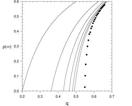
Figure 5: Local structure approximation for $p=0.2$. Solid lines represent consecutive orders of the local structure approximations, starting with $n=1$ (the leftmost curve), and ending with $n=6$ (the rightmost solid curve). The dots represent results of computer simulations ($p=0.2$, $R=1$).

As mentioned earlier, for $q=1$ and $R=1$, our model can be considered as a discrete realization of the contact process. For the contact process, theoretical studies as well as Monte Carlo simulations suggest that the phase transition occurs at $p_{c}$=0.3032 (Dickman and Jensen, 1991; Jensen and Dickman, 1993). The table below compares this result with our numerical simulations and local structure theory approximate results.

$n$	1	2	3	4	5	simulation	CP
$p_{c}$	1.00	1.00	0.70	0.62	0.55	0.48	0.3032

The discrepancy between discrete and continuous time versions of the contact process is understandable, since the synchronous dynamics of CA allows, for example, for one site to change its state from 1 to 0, and, at exactly the same time, for its neighbor to change its state from 0 to 1, something that does not occur in the continuous time model. We should stress at this point that although there are many analytical techniques developed to treat stochastic processes such as the contact process, none of them, in general, can be easily translated to the language of cellular automata theory, and the synchronicity of updating is usually the main source of difficulties. For example, the cluster approximation recently proposed for the contact process (Ben-Naim and Krapivsky, 1996) belong to this category.

On the other hand, when all transition probabilities are small, a single site of the lattice is rarely changed, and during most of the iterations of the CA it will remain in the same state. The updating, therefore, becomes more and more similar to asynchronous updating, and as a consequence, we can expect that the model should behave almost like the time-continuous contact process.

8 Conclusion

We have studied a probabilistic cellular automata model for the spread of innovations. Our results emphasize the importance of the range of the interaction between individuals. The innovation spreads faster when the range increases since increased connectivity between individuals reduces constrains on the exchange of information. Larger connectivity could be also achieved by increasing space dimensionality.

The range of interaction $R$ not only affects the growth rate, but in the region of parameter space $(p,q)$ bounded by the $R=1$ critical line and the mean-field line it can be a decisive factor for the asymptotic density of adopters $\rho(\infty)$. In this region, if $R$ is too small, $\rho(\infty)=0$, while for a sufficiently large connectivity $\rho(\infty)>0$.

References

- Bardos and Bessis (1980) Bardos, C. and Bessis, D., editors: Bifurcation Phenomena in Mathematical Physics and Related Topics. D. Reidel, Dordrecht, 1980.
- Bass (1969) Bass, F. M.: A new product growth for model consumer durables. Management Sciences 15:215, 1969.
- Ben-Naim and Krapivsky (1996) Ben-Naim, E. and Krapivsky, P. L.: Cluster approximation for the contact process. J. Phys. A: Math. Gen 27:L481, 1994.
- Boccara and Cheong (1992) Boccara, N. and Cheong, K.: Automata network sir models for the spread of infectious diseases in populations of moving individuals. J. Phys. A: Math. Gen. 25:2447, 1992.
- Boccara and Cheong (1993) Boccara, N. and Cheong, K.: Critical behaviour of a probabilistic automata network sis model for the spread of an infectious disease in a population of moving individuals. J.Phys. A: Math. Gen. 26:3707, 1993.
- Boccara et al. (1994) Boccara, N., Cheong, K., and Oram, M.: Probabilistic automata network epidemic model with births and deaths exhibiting cyclic behaviour. J. Phys. A: Math. Gen. 27:1585, 1994.
- Boccara et al. (1997) Boccara, N., Fukś, H., and Geurten, S.: A new class of automata networks. Physica D 103, 1997. To appear.
- Dickman and Jensen (1991) Dickman, R. and Jensen, I.: Time-dependent perturbation theory for nonequilibrium lattice models. Phys. Rev. Lett. 67:2391, 1991.
- Fukś and Boccara (1996) Fukś, H. and Boccara, N.: Cellular automata models for diffusion of innovations, in Instabilities and Nonequlibrium Structures VI, editor E. Tirapegui, Kluwer, Dordrecht, to appear.
- Gutowitz (1987) Gutowitz, H.: Local Structure Theory for Cellular Automata. Ph.D. thesis, Rockefeller University, New York, New York, 1987.
- Gutowitz et al. (1987) Gutowitz, H. A., Victor, J. D., and Knight, B. W.: Local structure theory for cellular automata. Physica D 28:18, 1987.
- Hägerstrand (1952) Hägerstrand, T.: The Propagation of Innovation Waves. Lund Studies in Geography. Gleerup, Lund, Sweden, 1952.
- Hägerstrand (1965) Hägerstrand, T.: On Monte Carlo simulation of diffusion. Arch. Europ. Sociol. 6:43, 1965.
- Harris (1974) Harris, T. E.: Ann. Prob. 2:969, 1974.
- Haynes et al. (1977) Haynes, K. E., Mahajan, V., and White, G. M.: Innovation diffusion: A deterministic model of space-time integration with physical analog. Socio-Econ. Plan. Sci. 11:23, 1977.
- Jensen and Dickman (1993) Jensen, I. and Dickman, R.: Nonequilibrium phase transitions in systems with infinitely many absorbing states. J. Stat. Phys. 48:1710, 1993.
- Liggett (1985) Liggett, T. M.: Interacting particle systems. Springer-Verlag, New York, 1985.
- Mahajan et al. (1990) Mahajan, V., Muller, E., and Bass, F. M.: New product diffusion models in marketing: A review and directions for research. Journal of Marketing 54:1, 1990.
- Mahajan and Peterson (1985) Mahajan, V. and Peterson, R. A.: Models for Innovation Diffusion. Number 07-048 in Quantitative Applications in the Social Sciences. Sage Publications, Beverly Hills, 1985.
- Rogers (1995) Rogers, E. M.: Diffusion of Innovations. The Free Press, New York, 1995.
- Wolfram (1986) Wolfram, S.: Theory and applications of cellular automata. World Scientific, Singapore, 1986.