Experiences with a simplified microsimulation
for the Dallas/Fort Worth area

Abstract

We describe a simple framework for microsimulation of city traffic. A medium sized excerpt of Dallas was used to examine different levels of simulation fidelity of a cellular automaton method for the traffic flow simulation and a simple intersection model. We point out problems arising with the granular structure of the underlying rules of motion.

Keywords: traffic, cellular automata, complex systems, parallel computing, route planning, shortest paths

1 Introduction

In recent time, traffic demand in metropolitan areas has largely exceeded capacity. Typical remedies such as the expansion of the road way system or road improvement do not work well anymore for various reasons: On the one hand communities cannot afford the increased costs of road construction, on the other hand there are political and environmental objections.

Therefore, computer simulation as a means of evaluating, planning, and controlling large traffic systems has gained considerable importance. The classical approach of traffic research consists of four steps: traffic generation, route planning, static assignment of routes onto the network, and evaluation. In recent years, more and more work has been invested to consider the dynamic aspects of these components. Especially the microsimulation part has taken great advantage of models developed in classical research areas such as physics, mathematics and computer science.

The failure of classical simulations to describe (and possibly predict) traffic was in part due to insufficient computational speed. One had the choice of simulating a rather large area (e.g. the metropolitan area of Los Angeles) at a low fidelity (vehicle densities instead of individual vehicles) or simulating a small excerpt (e.g. a suburb) at a high resolution. Only in recent years, it has become possible to use high-performance computers in conjunction with computationally efficient microsimulation models to simulate large areas at high resolution. Despite this advantageous development, execution speed still remains an issue. Especially since the traffic simulation consists of several stages, some of which have to be iterated several times to produce valid and consistent results. In this paper we would like to concentrate on the microsimulation portion.

In the next section, we present a simple model capable of executing a route set provided by a router. The functionality of the two major components, namely intersections and street segments, are outlined. The enforcement of speed limits and the usage of traffic lights are used to define four different levels of fidelity. We continue in section 3 by showing first results of the simulation obtained in conjunction with a TRANSIMS [1] case-study. Section 4 outlines the computational performance of the model as well as some aspects of its implementation on a parallel computer. We conclude by giving a short summary and some hints at future work.

2 Model

We use a simple representation of the underlying street network by transferring its basic elements (e.g. intersections and street segments) into their simulation counterparts, which we call nodes and edges. Each intersection is associated with a node. In contrast to their real-world counterparts, the simulation nodes do not have a micro-structure (e.g. shape, elaborate traffic light phases), but are reduced to very basic characteristics.

Each direction of street segment is represented by a directed edge connecting the respective nodes and pointing into the direction of traffic flow. This convention covers both one-way (e.g. exit/access ramps of freeways) and bi-directional street segments. Internally the traffic on each edge is simulated with a modified version of the cellular automaton of Ref. [2].

Next we will describe the two major components of our simulation.

2.1 Street Segments

The directed connection (edge) between two nodes is represented as a grid equivalent to the model by Nagel/Schreckenberg [2] and its two-lane extension [3]. The characteristics length, speed-limit, and number of lanes are used to adapt the cellular automaton (CA) model. The size of the grid is computed by using the grid-site length of 7.5 [meter] as a unit.

It is important to note that the characteristics mentioned so far are constant for the whole segment. Typical details like additional turning lanes in front of intersections are modeled by inserting additional nodes to split a given segment and assigning different parameters to the various parts.

Cellular Automaton Model

In case of only one lane the model of motion is equivalent to the original Nagel/Schreckenberg traffic CA [2] with an optional speed-limit $v_{sl}<v_{max}$. We would like to outline this model for the convenience of the reader.

The system consists of a one dimensional grid of $L$ sites with periodic boundary conditions. A site can either be empty, or occupied by a vehicle with an integer velocity zero to $v_{max}$. The velocity is equivalent to the number of sites that a vehicle advances in one update — provided that there are no obstacles ahead. Vehicles move only in one direction. The index $i$ denotes the index of a vehicle, $x(i)$ its position, $v(i)$ its current velocity, $v_{sl}(i)$ (“sl” for “speed limit”) its maximum speed imposed by a segment-specific speed-limit $pred(i)$ the index of the preceding vehicle, $gap(i):=x(pred(i))-x(i)-1$ the width of the gap to the predecessor. At the beginning of each time-step rules $S1\ldots S3$ (see below) are applied to all vehicles simultaneously (parallel update, in contrast to sequential updates which yield slightly different results). Then the vehicles are advanced according to their new velocities.

• IF $v(i)<v_{sl}(i)$ THEN $v(i):=v(i)+1\quad$ (S1)

• IF $v(i)>gap(i)$ THEN $v(i):=gap(i)\quad$ (S2)

• IF $v(i)>0$ AND $rand<p_{d}$ THEN $v(i):=v(i)-1\quad$ (S3)

S1 represents a constant acceleration until the vehicle has reached its maximum velocity $v_{sl}$. S2 ensures that vehicles having predecessors in their way slow down in order not to run into them. In S3 a random generator is used to decelerate a vehicle with a certain probability modelling erratic driver behavior. The free–flow average velocity is $v_{sl}-p_{d}$ (for $p_{d}\neq 1$).

In case of two lanes the model corresponds to the one described in [3]. For more than two lanes we extend the model using the same lane-changing rules. Collision of vehicles changing to the same neighboring site are prevented by a right-before-left lane priority (see also [4]).

Recently, the strictness of the CA model has been relaxed by maintaining only time as a discrete value, while using continuous values for location and velocity [5]. Modifications to the multi-lane rule-set yielded promising similarity to the lane-changing behavior found on German Autobahn through-ways [6, 7, 8].

Speed Limit

In contrast to the original CA model which assumed a maximum limit of approximately 120 km/h (freeway traffic), the speed limit within a city is usually lower. In order to match the speed-limits of the Dallas study area, for each segment we introduced a CA speed limit

$$v_{sl}=\lfloor v_{sl}^{real}/l_{site}+0.5+p_{d}\rfloor$$

where $v_{sl}$ is the CA speed limit given in sites per time-step, $v_{sl}^{real}$ the real speed limit given in meters per second, $l_{site}$ the CA site length given in meters, and $p_{d}$ the deceleration probability of the CA rule set. Moreover, $v_{sl}$ is forced to be in $[1\ldots v_{max}]$.

2.2 Intersections

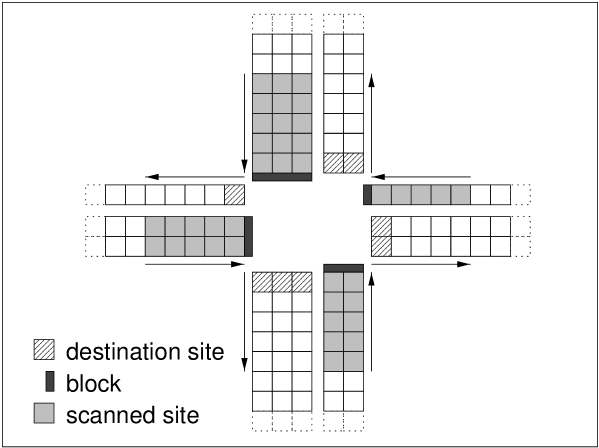
Figure 1: Geometry of an intersection

Intersections are modeled in a very simple fashion. The geometry is shown in figure 1. Although the figure gives the impression of an intersection having a spatial ’extent’, the simulation actually treats it as having no size at all. A vehicle is never inside the intersection, but either on the incoming lane or on one of the outgoing lanes. Therefore, the intersection does not have an explicit capacity unless incorporated into the network (e.g. transfer lanes at freeway-junctions [4]). An intersection of degree two (usually a node used to mimic the geometric trajectory of a street) is treated in a special way by connecting the incoming segments without any interruption visible to the vehicles.

All incoming lanes of each incoming segment are equivalent. At the very end of each incoming lane $v_{max}$ sites are scanned for vehicles before the usual rules of motion are applied. During each time-step, at most one vehicle per incoming lane of the source segment can be moved to one of the insertion sites of the destination segment. If possible the same lane is used on the destination segment. If the destination segment has fewer outgoing lanes than the incoming segment has incoming lanes the vehicle is inserted into the leftmost lane. If that site is occupied, the next neighboring site off to the right is checked until a vacant site is found or the right-most lane is reached. Note that the scanning of the incoming lanes is always done beginning at the site nearest to the intersection. That way, the order of the vehicles with respect to each other is not changed. In order to ensure unbiased processing of all incoming lanes, the scanning is done in a robin round fashion with respect to consecutive time-steps.

For a vehicle approaching the intersection there are two alternatives: either it is absorbed from the scanning area and inserted into the destination segment or it proceeds according to its CA rules of motion. Due to block at the end of the lane (or earlier due to other preceding travelers) it will eventually stop. This behavior is important to model the spill backs in real world traffic. The queues are resolved as one would expect: As soon as the situation on the destination lane(s) improves, vehicles are removed one by one starting at the site nearest to the block. Note that a vehicle may be blocked by other vehicles (having a different destination) although its destination segment is vacant.

Approach and turning behavior

In contrast to other traffic simulations with resolution at city-street level, we do not model a special behavior for vehicles while approaching or transversing intersections. In the implementation described in this paper, all incoming lanes are equivalent. This was done for two reasons. First, modeling detailed approach and turning behavior requires extensive geometric information which is often not available or not consistent. Second, the current rules of motion show a quickly decreasing lane-changing probability as soon as the density exceeds a certain threshold. This is mainly due to a strict ’look-back’ rule which checks for following traffic on the neighboring lane. In contrast to freeway conditions, where this rule maintains the desired traffic jam waves (see [3]), in this context, it would prevent proper lane-changing. This again would result in vehicles queuing up, since they could not change to their respective turning lanes [9].

Traffic Lights

Traffic lights are modeled by activating the scanning mechanism for the duration of the green phase and deactivating it for the length of the non-green-phase (which includes both the red phase and transition phases). Since there is only one phase per incoming segment, any direction-specific phasing information is averaged over all directions weighted by the number of active lanes into the respective direction.

Note that due to this averaging, the complete phase cycles $T_{rg}=T_{g}+T_{r}$ (green phase + red phase) of the incoming segments may differ from each other, resulting in a continuous phase shift. This is different from real world traffic light installations where the starting time is usually defined by taking a multiple of $T_{rg}$ and adding a relative offset.

Interferences

Two types of interference can occur at an intersection: (a) vehicles that have to obey right of way must wait for gaps in the crossing or oncoming traffic stream, and (b) vehicles that have right of way are obstructed by others blocking the intersection. In the simplest version of our intersection of neither of these interferences is handled. However, it is simple to force a reduced throughput through the intersection by examining the overall occupancy of the $v_{max}$ last sites of all outgoing segments and introducing an additional transfer probability. This probability would be one if all sites in the examined area are vacant, zero if all occupied with a functional (possibly linear) transition between the two extremes.

2.3 Plan Following

For each simulation run all plans can be regarded as static. For the time being, we do not perform any on-line re-routing. A plan-set is generated from an activity set consisting of a source plus a departure time on the one hand and destination on the other hand. The plan-set used for the study presented here (also referred to as plan-set 11) is a very preliminary plan-set which was generated in the course of the Dallas/Fort Worth case study of TRANSIMS. Since this paper concentrates on microsimulation aspects, describing the method how plan-sets were obtained goes beyond the scope of this paper. Work on plan-sets in the context of the same case study can be found in Refs. [10, 11].

The plan-sets in TRANSIMS are sequences of links plus estimates when these links will be reached. From this, one can calculate when every driver expects to be on a certain link. In consequence, one can calculate the complete time dependent demand structure, which would correspond to the traffic which would happen if everybody could act according to her expectations.

This demand structure is best displayed in terms of the ratio of flow demand to capacity, also called V/C ratio. If the V/C ratio is exactly one, the number of vehicles which are planning to use a certain link is equal to the maximum number of vehicles the link can let through. If the V/C ratio is larger than one, then the number of vehicles in excess of the capacity will not be able to get through and will be queued up at the entrance of the link. This means that these vehicles will not be at other links downstream when they expected, so that the demand structure downstream of a congested link (i.e. V/C $>1$) becomes wrong. From this argument it becomes immediately clear that one has to run the microsimulation to obtain dynamically correct traffic patterns.

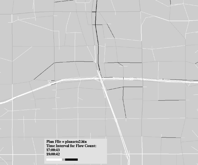
Figure 2: V/C-ratios. White links mean that demand is lower than capacity ($V/C<1$); for gray links demand is between capacity and two times capacity ($1\leq V/C<2$); for black links demand is larger than two times capacity ($2\leq V/C$)

Fig. 2 shows a graphical display of the demand structure of a plan-set which is similar to the one used for the simulation runs in this paper.

All plan-sets are computed for the whole Dallas/Forth-Worth area which means that all routes have to be restricted to the study area if only that portion of the map is simulated. The truncation of the plans is done in a straight-forward way: any route that contains at least one segment within the study-area will be part of the restricted plan set. Its departure will be delayed by the amount of time that the vehicle would spent outside the study-area before it reaches the first segment within the simulation area. For all edges transversed up to entry, we use the cruising velocities assumed by the planner.

After the start of the simulation, route-plans are executed as follows: (a) At the time-step given by the departure-time, a vehicle is created at the departure node (source) of the route. (b) The vehicle is inserted into a queue associated with the source. (c) Each time-step the queue is scanned for pending vehicles. If possible, the vehicle is removed from the queue and inserted into the first segment, from where it starts following its route-plan. (d) As soon as it reaches the destination, the vehicle is removed from the segment. The travel time is recorded for statistical evaluation.

Note that all vehicles try to execute their route-plans independent of the actual traffic conditions that they encounter along their way. In heavily congested areas, vehicles often spill back across intersections because they cannot enter their next respective destination segments. In combination with the grid-oriented characteristics of the CA model, this can result in complete grid-locks of the simulation area, which cannot be resolved anymore within the current rule-set. This artifact will be discussed in paragraph 3.2

Sources and Sinks

Vehicles are inserted into and removed from streets at special sites acting as sources and sinks. A source consists of $n_{source}$ consecutive sites (in each lane), which all have to be vacant before a vehicle can be inserted. The location of a source (or sink) is usually defined by intersections with the lower level street network that have not been included into the simulation network. Thus, the sources serve as aggregate feeding facilities.

The maximum throughput source is one vehicle per time-step and lane, which is well above the rates seen in reality. In fact, these values will never be reached, since the CA model usually restricts the throughput of a lane to about 1600-1800 vehicles per hour. Remember that the actual feeding frequency of a source, however, is determined by the number of plans originating from it.

A sink consists of $v_{max}$ consecutive sites (on each lane) which are scanned for vehicles that have reached their destination. This is to make sure that every vehicle passing the sink spends at least one time-step within this range. Since every vehicle is deleted without delay, the sink can — using the inverse argument as above — absorb all incoming traffic without generating a spill–back.

3 Simulation Results

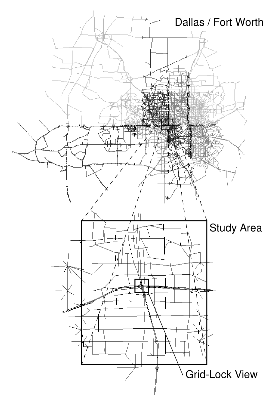
Figure 3: Maps used in simulation. The different shades of gray in the Dallas/Fort Worth map correspond to the mapping to different processors of the parallel computer topology.

All figures shown in this section are based upon data sets used in a case study of the TRANSIMS [12] project. We used two maps (see 3): the complete Dallas/Fort Worth Area and a small excerpt of the latter called study area. The study area maps comprises all streets except small ones in residential areas and similar areas. The large map further contains all minor and major arterials for Dallas and all major arterials for Forth Worth.

The plan-sets which we had available contained only trip departure times between 7 a.m. and 10 a.m. of which we selected those between 7 a.m. and 8 a.m. as period of interest. We thus started the simulation at 7 a.m. and let it run at least until 8 a.m. After that, the simulation either terminated when (a) 99% of all route-plans had been executed, or (b) a grid-lock was detected. In this context we assume the system to be grid-locked if the number of vehicles in the system is constant for more than 600 time-steps. For the CA model we used the deceleration probability of $p_{d}=0.3$ in all simulations.

During the simulation we keep track of: the number of vehicles inserted so far, the number of vehicles currently in the network, and the number of vehicles that have reached their destination. Upon arrival of each vehicle we store the estimated travel time (computed by the router beforehand) and the actual travel time. These can be compared to check the prediction quality of the router.

Except for the curves depicting the number of vehicles in the study-area (figure 7), we considered only vehicles that arrived before time-step 1800. Also, all curves have been aggregated over 10 simulation-runs (using different random seeds). They have been normalized by the respective number of vehicles that have reached their destinations before time-step 1800. Moreover the area underneath each curve has been normalized to one.

3.1 Levels of Fidelity

It must be the principal goal of a traffic simulation within a cellular automaton context to keep the interaction rule-set as small as possible. This has two advantages: (a) The number of parameters will be small, which reduces the probability of artifacts and makes the model more credible, if it can be successfully validated using those parameters. (b) A simple rule-set usually results in efficient coding, which is essential, considering the before-mentioned necessity of iteration and statistical averaging.

We examine different levels of fidelity by simulating the same plan-set after activating different combinations of characteristics of intersections and street segments which were described above. We ran simulations for the combinations listed in table 1.

short name	lf	sl	tl	hf	rl
long name	low fidelity	speed limits	traffic lights	high fidelity	reduced lights
speed limit	no	yes	no	yes	yes
traffic lights	no	no	yes	yes	$q_{r}$

Table 1: Parameters (bottom rows) defining the fidelity (right columns) of the simulation: In case of an active speed-limit the maximum velocity $v_{max}$ is reduced from its original value of 5 to a segment-specific value. In case of active traffic lights, the transfer at intersections is decreased by introducing periodic red phases during which some of the incoming segments are blocked. Reduced non-green phases ($q_{r}$) are discussed in paragraph 3.3.

Delay of arrival

Figure 4: Distribution of relative delays for plan-set 11

Figure 5: Running average of relative delays for plan-set 11

Since upon arrival of each vehicle its actual travel time $t_{actual}$ is recorded, we could compute the distribution of relative delay $d$

$$d=\frac{t_{actual}-t_{scheduled}}{t_{scheduled}}$$

with respect to the scheduled trip time $t_{scheduled}$ forecast by the router. Note that negative values denote early arrivals. Figure 4 shows the results for plan-set 11 in all fidelities. It is obvious that in mode lf (due to the missing speed-limit) route-plans are executed much too fast. There are hardly any late-comers at all. In modes sl and tl the peak is already shifted towards zero delays but still biased. Mode hf generates a distribution which peaks almost exactly at zero delay. The average, however, is shifted towards positive delays. This can be verified in figure 5, which displays the running average (over the latest 1000 vehicles) of the relative delay. As can be seen, in the uncongested regime the travel times of the microsimulation are in general shorter than what the planner had expected. Yet, in highly congested situations, travel times in the microsimulation become longer than what the planner had expected.

We have to point out that it cannot be the goal of the dynamic microsimulation to reproduce static results forecast by the planner. These comparisons only serve as a consistency-check. It is to be expected that results of the microsimulation will considerably differ, e.g. in places where the implicit aggregation of the planner smoothes over sudden peaks in traffic load.

Trip Duration

Figure 6: Distribution of trip duration

Figure 6 depicts the distribution of trip durations for all fidelities. As expected mode lf has its peak shifted far left towards small trip durations. Mode tl has a significant peak at approximately 50 [sec], where it reaches the same value as lf. This is due to the fact that the probability of encountering a traffic light is a very small for short trips, rendering modes lf and tl equivalent in that regime. Modes tl and hf have a very slow descent towards large trip durations due to grid-locks. The curve of planned trip duration is best matched by mode sl.

3.2 Reproducibility and Grid-Locks

Figure 7: Vehicles in study area for plan-set 11

Since the CA model contains a stochastic element, we receive a unique evolution of the simulation for each seed of the random number generator. In a sub-critical system the network is able to transport all vehicles (albeit with delay) so that all runs will look similar on a macroscopic level. In a system with a network throughput incapable of handling the loading, the system will most likely grid-lock (see below). Between the two extremes we find a regime in which the specific configuration may either block or not block. Figure 7 depicts the number of vehicles which are in the study-area at a given time-step. Fidelities lf and sl belong to the sub-critical regime. Both curves reach a plateau (at 4500 vehicles after time-step 500 for lf and at 10000 vehicles after time 2500 for sl) after an initial loading phase representing an equilibrium between the insertion and deletion rates of vehicles. After the loading phase all remaining vehicles are discharged within 400 time-steps for lf and within 900 time-steps for sl.

Modes tl and hf belong to the super-critical regime. They never reach an equilibrium between insertion and deletion during the loading phase; and the plateau after the loading of the network is due to grid-lock.

See Ref. [13] for a similar (albeit much smaller scale) investigation on the relation between network loading and network throughput.

Grid-locks

Figure 8: Grid-lock

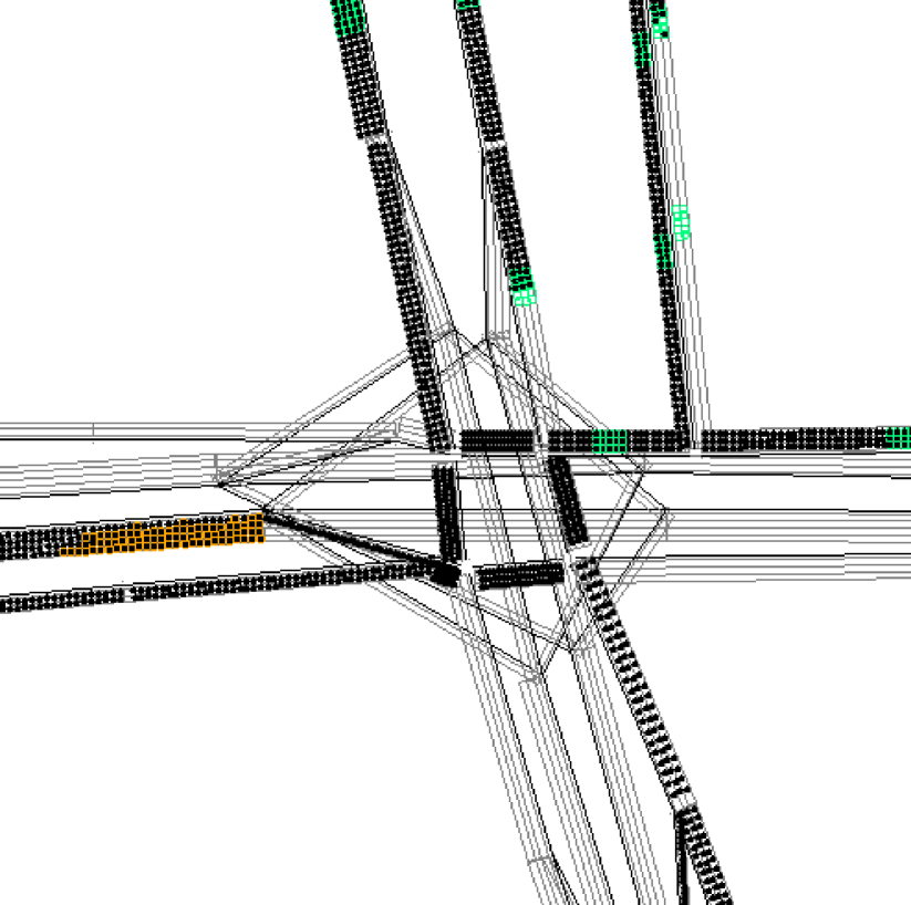
Figure 9: Grid-lock in study-area (plan 11, mode hf)

A grid-lock situation can be determined by a horizontal line after time-step 3600 (e.g. the end of vehicle insertion). This is caused by closed loops in the traffic network in which all sites are occupied. Figure 8 depicts a simplified intersection. In the left half traffic is already dense, though not grid-locked. Due to high demand and the red-phases at the intersection, the segments of the loop are no longer cleared. In the right half the whole loop is blocked: the first vehicle in each lane is forced to make a right turn into another lane which is also blocked. This phenomenon (in its strict form) cannot be seen in real-world traffic, because drivers move out of the lanes and pass on the on-coming lane or they abandon their current route and choose a detour. Figure 9 shows a screen-shot of a simulation run with plan-set 11 in mode hf. Vehicles are represented by dark dots, lane boundaries by grey lines. Right at the center, there is a small grid-locked loop blocking traffic from all incoming directions.

3.3 Reduced Non-Green Phase Length

Figure 10: Distribution of relative delay of plan-set 11 (different $q_{r}$)

Figure 11: Vehicles in study area (different $q_{r}$)

Figure 12: Vehicles in study area ($q_{r}=0.55,0.6,0.65,0.7$)

Above we have seen cases of sub-critical and super-critical loading of the network. Although the respective models are defined by different types of rule-sets, they can be regarded as two specific cases of a more general rule-set (called rl) in which in the effective red-phase $T_{r,eff}$ is computed by multiplying the original phase-length $T_{r}$ by a certain factor $q_{r}\in[0\ldots 1]$. Consequently, $q_{r}=0$ represents mode sl while $q_{r}=1$ represents mode hf.

We have made several runs for different values of $q_{r}$ between 0 and 1. Both figures 10 and 11 show a smooth transition between modes sl and hf (for $0.6$ and $0.65$ blocking and non-blocking representatives were chosen) as far as delay and trip duration are concerned. Values below $0.6$ show a secure sub-critical (no grid-locks), and values above $0.65$ a secure super-critical behavior. For $0.6$ and $0.65$ the system has a certain chance of reaching a grid-lock (1 out of 10 runs for $q_{r}=0.6$ and 5 out of 10 for $q_{r}=0.65$), which can better be seen in figure 12.

A similar effect was reported for simple 2-dimensional grid models [14, 15, 16], except that in these studies the overall density was changed instead of the efficiency of the network components. Intuitively, the grid-lock effect seems to be the same. Yet, further investigations will be necessary to understand in how far simple models on a 2-dimensional grid can indeed offer insight for real-world city traffic, which is admittedly happening in 2-dimensional space but is composed of traffic on 1-dimensional links. It is for example unclear if dynamical critical exponents are the same.

4 Performance and Implementation

Map	Study Area				Dallas / Fort Worth
Architecture	SUN Sparc 20				8 SUN Sparc 20
Resolution	lf	sl	tl	hf	hf
MOSPS (average)	0.015	0.032	0.077	0.092	0.095
MOSPS (max)	0.022	0.045	0.125	0.153	0.156
MUPS (average)	0.704	0.689	0.788	0.647	4.880
MUPS (max)	2.020	1.989	1.953	1.908	8.950

Table 2: Performance

We measure performance in units of the so-called real-time-ratio (RTR). An RTR of 1.0 means that one simulation second (corresponding to one simulation time-step) takes one wall-clock second to execute. Larger values denote faster simulations. Other interesting measurement units are the number of vehicles (MOSPS = million object seconds per second) and the number of sites (MUPS = million updates per second) that can be updated in one wall-clock second. Table 2 contains an overview of all performance benchmarks. Note that the MOSPS values are density-dependent which results in larger numbers for grid-locking modes tl and hf since the network contains up to three times as many vehicles.

4.1 Study Area (1 CPN)

Figure 13: Performance for study area map

The map excerpt representing the study-area comprises of 374 intersections (93 of which have traffic lights) and 528 segments (142 of which are one-way). The total length of the roadway summed over all lanes is 1154 [kilometer] or 153,022 sites. All runs were done on single Sparc Stations 5 and 20. Figure 13 shows the performances for all fidelities during the simulation. The RTR drops rapidly until approximately 5000 vehicles are in the system and more slowly until the end of the vehicle insertion phase is reached. As expected, the high fidelity mode is the slowest. The difference between the modes is minimal and the RTR does not drop far below four during the main portion of the simulation.

4.2 Dallas/Fort Worth (8 CPN)

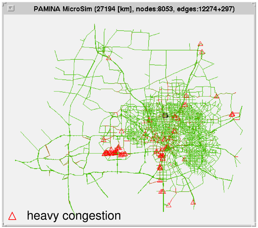
Figure 14: Screen-shot of congestion in Dallas/Fort Worth area after 9 minutes

The map representing the whole Dallas/Fort Worth area comprises of 8053 intersections (93 of which have traffic lights = those in the study area) and 12,274 segments (4772 of which are one-way and 366 of which were split across CPN boundaries). The total length of the roadway summed over all lanes is 27,194 kilometers or 3,608,781 sites.

The whole Dallas/ Fort Worth Area was simulated on a SUN Sparc workstation cluster using 8 machines coupled via optical LAN (see figure 3). The RTR was approximately 1.0 between time-steps 500 and 1200 when the number of vehicles reached its maximum at 128,000 vehicles. Unlike before, the route set contained all routes through the region. Disk space limitations forced us to shorten the insertion period to 20 minutes: Using the current TRANSIMS plans format, plans for one hour would have needed close to one GByte of disk space. The results presented here shall thus only serve as a proof of feasibility. For the time being, a more detailed evaluation is not reasonable, since the underlying network was not homogeneous: outside Dallas only major arterials were used to hold the traffic which is usually spread over the topmost two or three street hierarchies. We experienced extreme clogging of those arterials. A good estimate for the computational speed of the overall detailed network can be obtained if the overall length (in lane kilometers ) of the network is known. Usually the factor between a high-fidelity and a arterial network is about 3 to 5 which would still result in a RTR of about 0.2-0.3 for this type of architecture.

Figure 14 depicts the network after 9 minutes of loading. The small triangles denote heavy congestion. Note the heavy congestion along the southbound and westbound axes.

Parallelization

We use a geometrical domain decomposition approach to distribute the street network among the CPN. A recursive orthogonal bisection is used to determine the sub-networks which are connected through boundaries located in the middle of street-segments. Before each time-step boundary information consisting of vehicle state information is passed to neighboring CPN with message passing routines (PVM[17]). The time-step itself is independently performed in parallel on all machines. For a more detailed description of parallelization scheme see [4, 18].

5 Summary, Conclusion and Future Work

We have presented a simple microsimulation model for city traffic. The goal was to find a simple extension to the original traffic CA which can handle city-like intersections. In its “high fidelity” mode, the proposed intersection model reaches satisfactory results while maintaining a high computational speed.

We have pointed out the danger of grid-locks which are due to the granular structure in combination with static route-plans. It will be necessary to include on-line re-routing to reduce the risk of grid-locks. Also, the impact of travellers’ information systems can only be examined, if route-plans are no longer static for the duration of one simulation run.

We showed that the a simple parameter like $q_{r}$ can be used to fine-tune the performance of the intersection throughput. For $q_{r}\simeq 0.6$ the curves for relative delay were optimal while the behavior with respect to grid-locking was improved considerably.

In future, we will repeat the runs with more detailed maps: on the one hand, it is necessary to determine what fidelity the enclosing network (that is Dallas/Fort Worth without the study area) will have to have to suppress the congestion outside the study area. On the other hand, the map of the study area which was used for all simulations in this paper did still not include all street levels. The system actually was missing some of its road capacity located in residential areas. The sources and sinks acted as devices which aggregated (or disaggregated respectively) the traffic flow close to insertion and deletion points. As a result, the existing streets are not loaded as homogeneously as they would be, if all access points (sources or sinks) only represented their immediate vicinities.

Running the simulation multiple times reveals information about the robustness of traffic flow along specific routes. It will be interesting to classify street segments by the fluctuation of traffic flow data collected over several runs. Areas of high fluctuations may be good candidates to install intelligent traffic control mechanism to prevent congestion using on-line traffic counts. Another interesting aspect would be the examination of damage spreading in a complex traffic system: reducing the efficiency or blocking an intersection for a certain period will cause traffic jams moving away from the origin of the disturbance and possibly changing the fluctuation structure in another region of the network.

References

- [1] K. Nagel, C. Barrett, and M. Rickert. Parallel traffic microsimulation by cellular automata and application for large scale transportation modeling. Technical report, TSA-DO/SA, Los Alamos National Lab, New Mexico, USA, and Santa Fe Institute, Santa Fe, New Mexico, USA, and Center for Parallel Computing, University of Cologne, Germany, 1996.
- [2] K. Nagel and M. Schreckenberg. A cellular automaton model for freeway traffic. J. Phys. I France, 2:2221, 1992.
- [3] M. Rickert, K. Nagel, M. Schreckenberg, and A. Latour. Two lane traffic simulations using cellular automata. Physica A, 231:534, 1996.
- [4] M. Rickert and P. Wagner. Parallel real-time implementation of large-scale, route-plan-driven traffic simulation. Int.J.Mod.Phys. C, 7:133–153, 1996.
- [5] S. Krauss, P. Wagner, and C. Gawron. A continuous limit of the Nagel-Schreckenberg model. Phys. Rev. E, 54:3707, 1996.
- [6] K. Nagel, P. Wagner, and D.E. Wolf. in preparation, 1997.
- [7] P. Wagner, K. Nagel, and D.E. Wolf. Realistic multi-lane traffic rules for cellular automata. Physica A, 234:687, 1997.
- [8] P. Wagner. Traffic simulations using cellular automata: Comparison with reality. In D.E.Wolf, M.Schreckenberg, and A.Bachem, editors, Traffic and Granular Flow, Singapore, 1996. World Scientific.
- [9] C.L. Barrett. Personal communication.
- [10] M. Marathe, D. Anson, M. Stein, M. Rickert, K. Nagel, and C.L. Barrett. Engineering the route planner for the Dallas case study. In preparation.
- [11] K. Nagel and C.L. Barrett. Using microsimulation feedback for trip adaptation for realistic traffic in Dallas. International Journal of Modern Physics C, this issue.
- [12] TRANSIMS URL. http://www-transims.tsasa.lanl.gov/.
- [13] C.L. Barrett and M.A. Wolinsky. Incident-induced flow anomaly analysis and detection testbed final report: Design and concept demonstration. Technical report, Los Alamos National Laboratory, TSA-DO/SA, 1995.
- [14] Cuesta J A, Martínez F C, Molera J M, and Sánchez A. Phase transitions in two-dimensional traffic flow models. Phys. Rev. E, 48(6):R4175–R4178, 1993.
- [15] J. Freund and T. Pöschel. A statistical approach to vehicular traffic. Physica A, 219(1–2), 1995.
- [16] T Nagatani. Effect of traffic accident on jamming transition in traffic-flow model. J. Phys. A, 26(19):L1015, 1993.
- [17] PVM URL. http://www.epm.ornl.gov/pvm/pvm_home.html.
- [18] M. Rickert, P. Wagner, and Ch. Gawron. Real-time traffic simulation of the German Autobahn Network. In Proceedings of the 4th PASA Workshop, 1996. in press.
- [19] URL. http://www.zpr.uni-koeln.de/Forschungsverbund-Verkehr-NRW/.