Cellular Automata Models for Diffusion of Innovations

Abstract

We propose a probabilistic cellular automata model for the spread of innovations, rumors, news, etc. in a social system. The local rule used in the model is outertotalistic, and the range of interaction can vary. When the range $R$ of the rule increases, the takeover time for innovation increases and converges toward its mean-field value, which is almost inversely proportional to $R$ when $R$ is large. Exact solutions for $R=1$ and $R=\infty$ (mean-field) are presented, as well as simulation results for other values of $R$. The average local density is found to converge to a certain stationary value, which allows us to obtain a semi-phenomenological solution valid in the vicinity of the fixed point $n=1$ (for large $t$).

1 Introduction

Diffusion phenomena in social systems such as spread of news, rumors or innovations have been extensively studied for the past three decades by social scientists, geographers, economists, as well as management and marketing scholars. Traditionally, ordinary differential equations have been used to model these phenomena, beginning with the Bass model [1] and ending with sophisticated models which take into account learning, risk aversion, nature of innovation etc. [9, 10, 11]. Models incorporating space and spatial distribution of individuals have been also proposed, although most research in this field has been directed to the refining of discrete Hagerstrand models [5, 6] and to constructing partial differential equations similar to diffusion equations known to physicists [7].

Diffusion of innovations (we will use this term in a general sense, meaning not only innovations, but also news, rumors, new products etc.) is usually defined as a process by which the innovation “is communicated through certain channels over time among the members of a social system” [11]. In most cases, these communication channels have rather short range, i.e. in our decisions we are heavily influenced by our friends, family, coworkers, but not that much by unknown people in distant cities. This local nature of social interactions makes cellular automata a convenient tool in modeling of diffusion phenomena. In fact, epidemic models formulated in terms of automata networks have been succesfully constructed in recent years [2, 3, 4].

In what follows, we will propose a model for the spread of innovations formulated in terms of probabilistic cellular automata, and investigate the role of the range of interaction in the diffusion process.

Let us define a symbol set ${\cal G}=\{0,1,...k-1\}$ and a bisequence over ${\cal G}$ which is a function on ${\rm Z}$ (the set of all integers) to ${\cal G}$, that is, $s:{\rm Z}\to{\cal G}$. The set of all bisequences over ${\cal G}$, i.e. ${\cal S}={\cal G}^{{\rm Z}}$, is called the configuration space, and its elements are called configurations. The mapping $T:{\cal S}\to{\cal S}$ defined by $[T(s)](i)=s(i+1)$ for every $i\in{\rm Z}$ is called the (left) shift.

Let $F:{\cal S}\to{\cal S}$ be a continuous map commuting with $T$. In general, a cellular automaton (CA) [12] is a discrete dynamical system defined by

$$s_{t+1}=F(s_{t}).$$ (1)

As proved in [8], in this case one can always find a local mapping such that the value of $s_{t+1}(i)$ depends only on a finite number of neighboring $s_{t}(j)$ values. In the remaining part of this paper we will only consider 2-state probabilistic cellular automata, with a dynamics such that $s_{t+1}(i)$ depends on $s_{t}(i)$ and $\sigma_{t}(i)$, where

$$\sigma_{t}(i)=\sum_{n=-\infty}^{\infty}s_{t}(i+n)p(n),$$ (2)

and $p$ is a nonnegative function satisfying

$$\sum_{n=-\infty}^{\infty}p(n)=1.$$ (3)

In the simplest version of our model, the sites of an infinite lattice are all occupied by individuals. The individuals are of two different types: adopters ($s_{t}(i)=1$) and neutrals ($s_{t}(i)=0$). Once an individual becomes an adopter, he remains an adopter, i.e. his state cannot change. At every time step, each neutral individual can become an adopter with a probability depending on the parameter $\sigma$. In this paper we will assume that this probability is equal to $\sigma$.

The model can be viewed as a probabilistic cellular automaton with probability distribution

$$P(s_{t+1}(i)=0) = \big{(}1-s_{t}(i)\big{)}\big{(}1-\sigma_{t}(i)\big{)}$$ (4)

$$P(s_{t+1}(i)=1) = 1-\big{(}1-s_{t}(i)\big{)}\big{(}1-\sigma_{t}(i)\big{)}$$ (5)

The transition probability $P_{b\leftarrow a}$ is defined as

$$P_{b\leftarrow a}=P(s_{t+1}(i)=b|s_{t}(i)=a),$$ (6)

and represents the probability for a given site of changing its state from $a$ to $b$ in one time step. The transition probability matrix in our case has the form

$$\mathbf{P}=\left[\begin{array}[]{cc}P_{0\leftarrow 0}&P_{0\leftarrow 1}\\ P_{1\leftarrow 0}&P_{1\leftarrow 1}\end{array}\right]=\left[\begin{array}[]{cc}1-\sigma_{t}(i)&0\\ \sigma_{t}(i)&1\end{array}\right].$$ (7)

Subsequently, we will consider an uniform outertotalistic neighborhood of radius $R$, with the parameter $\sigma$ defined as

$$\sigma_{t}(i)=\frac{1}{2R}\left(\sum_{n=-R}^{-1}s_{t}(i+n)+\sum_{n=1}^{R}s_{t}(i+n)\right).$$ (8)

$\sigma$ is then a local density of adopters over $2R$ closest neighbors. This choice of $\sigma$, although somewhat simplistic, captures some essential features of a real social system: the number of influential neighbors is finite and these neighbors are all located within a certain finite radius $R$. Opinions of all neighbors have equal weight here, which is maybe not realistic, but good enough as a first approximation. Let $n_{t}$ be the global density of adopters at time $t$ (i.e. number of adopters per lattice site), and $m_{t}=1-n_{t}$. Since $P_{1\leftarrow 1}=1$, the number of adopters increases with time, and $\lim_{t\rightarrow\infty}n_{t}=1$. If we start with a small initial density of randomly distributed adopters $n_{0}$, $n_{t}$ follows a characteristic S-shaped curve, typical to many growth processes. The curve becomes steeper when $R$ increases, and if $R$ is large enough it takes only a few time steps to reach a high $n$ (e.g. $n=0.99$). Figure 1 shows some examples of curves obtained in a computer experiment with a lattice size equal to $10^{5}$ and $n_{0}=0.02$.

Figure 1: Density of adopters (vertical axis) as a function of time (horizontal axis) for several values of radius $R$

2 Exact Results

Average densities $n_{t+1}$ and $m_{t+1}$ can be obtained from previous densities $n_{t}$ and $m_{t}$ using the transition probability matrix ( $\langle\rangle$ denotes a spatial average)

$$\left(\begin{array}[]{c}m_{t+1}\\ n_{t+1}\end{array}\right)=\left[\begin{array}[]{cc}\langle P_{0\leftarrow 0}\rangle&\langle P_{0\leftarrow 1}\rangle\\ \langle P_{1\leftarrow 0}\rangle&\langle P_{1\leftarrow 1}\rangle\end{array}\right]\left(\begin{array}[]{c}m_{t}\\ n_{t}\end{array}\right),$$ (9)

hence:

$$n_{t+1}=n_{t}\langle P_{1\leftarrow 1}\rangle+(1-n_{t})\langle P_{1\leftarrow 0}\rangle,$$ (10)

and using (7) we have

$$n_{t+1}=n_{t}+(1-n_{t})\langle\sigma_{t}(i)\rangle.$$ (11)

This difference equation can be solved in two special cases, $R=1$ and $R=\infty$.

If $R=1$, only three possible values of local density $\sigma$ are allowed: $0,\frac{1}{2}$ and $1$. The initial configuration can be viewed as clusters of ones separated by clusters of zeros. Only neutral sites adjacent to a cluster of ones can change their state, and they will become adopters with probability $\frac{1}{2}$. All other neutral sites have local density equal to zero, therefore they will remain neutral, as shown in an example below (sites that can change are underlined):

$\cdots$ 1 0 0 0 1 1 0 0 0 0 1 1 $\cdots$

This implies that the length of a cluster of zeros will on average decrease by one every time step, i.e.

$$M(s,t+1)=M(s+1,t),$$ (12)

where $M_{(}s,t)$ denotes a number of clusters of zeros of size $s$ at time $t$, and furthermore

$$M(s,t)=M(s+t,0).$$ (13)

For a random configuration with initial density $n_{0}$, the cluster density is given by

$$M(s,0)=(1-n_{0})^{s}n_{0}^{2},$$ (14)

hence

$$M(s,t)=(1-n_{0})^{s+t}n_{0}^{2}.$$ (15)

The density of zeros can be now easily computed as

$$m_{t}=\sum_{s=1}^{\infty}sM(s,t)=(1-n_{0})^{t+1},$$ (16)

and finally

$$n_{t}=1-(1-n_{0})^{t+1}.$$ (17)

Using the above expression, we obtain

$$n_{t+1}=n_{t}+(1-n_{t})n_{0},$$ (18)

Comparing with (11) this yields $\langle\sigma_{t}\rangle=n_{0}$, i.e. the average probability that a neutral individual adopts the innovation is time independent and equal to the initial density of adopters.

When $R\rightarrow\infty$, local density of ones becomes equivalent to the global density, thus in (11) we can replace $\langle\sigma_{t}\rangle$ by $n_{t}$:

$$n_{t+1}=n_{t}+(1-n_{t})n_{t},$$ (19)

or

$$1-n_{t+1}=(1-n_{t})^{2}.$$ (20)

Hence

$$n_{t}=1-(1-n_{0})^{2^{t}}.$$ (21)

Note that this case corresponds to the mean-field approximation, as we neglect all spatial correlations and replace the local density by the global one.

3 Simulations

Solutions obtained for the limiting cases discussed in the previous section suggest that in general the density of adopters might have the form

$$n_{t}=1-(1-n_{0})^{f(t,R)},$$ (22)

where $f$ is a certain unknown function satisfying $f(t,1)=t+1$ and $f(t,\infty)=2^{t}$. Plots of this function for several different values of $R$ are shown in Figure 2. They were constructed by measuring

Figure 2: Plots of $f(t,R)$ (vertical axis) as a function of time (horizontal axis) for several values of radius $R$.

$n_{t}$ and using

$$f(t,R)=\frac{\ln(1-n_{t})}{\ln(1-n_{0})}.$$ (23)

Two apparent features of $f(t,R)$ can be observed: for every finite $R$, the function $f(t,R)$ becomes asymptotically linear, and the slope of the asymptote increases with $R$. This slope can be defined as a limit

$$a(R)=\lim_{t\rightarrow\infty}\frac{\ln(1-n_{t})}{t\ln(1-n_{0})},$$ (24)

and as Figure 2 indicates, $a(R)$ increases with $R$.

Since $f(t,\infty)=2^{t}$, we can “rescale” $f(t,R)$ and introduce $g(t,R)=2^{-t}f(t,R)$, so that $\lim_{R\rightarrow\infty}g(t,R)=1$. Several sample graphs of $g(t,R)$ as a function of $R$ for different values of $t$ are shown in Figure 3.

Figure 3: Plots of $g(t,R)=2^{-t}f(t,R)$ (vertical axis) as a function of radius $R$ (horizontal axis) for several values of time $t$.

This set of graphs reveals certain regularity of $g(t,R)$, namely the shape of the $g(t,R)$ for a given $t$ is the same as the shape of $g(t+1,R)$ with vertical axis rescaled by a factor 2, i.e. $g(t+1,2R)=g(t,R)$. In terms of our original function $f$ this becomes

$$f(t+k,2^{k}R)=2^{k}f(t,R),$$ (25)

where k is a positive integer. This condition is more accurate for larger $R$, although we found it well satisfied even for rather small $R$ (less than 10). It is seriously violated only for $R=1$, when $f(t,1)=t+1$.

Combining (11) and (22), we can express average local density $\sigma$ in terms of $f(t,R)$:

$$\langle\sigma_{t}\rangle=1-(1-n_{0})^{f(t+1,R)-f(t,R)}.$$ (26)

Since $f(t,R)$ is linear for large $t$, the average local density must become time-independent for large $t$, and therefore

$$\lim_{t\rightarrow\infty}\langle\sigma_{t}\rangle=1-(1-n_{0})^{a(R)}.$$ (27)

This limit will be referred to as $\langle\sigma_{\infty}\rangle$. The average local density converges to $\langle\sigma_{\infty}\rangle$ rather quickly. For example, when $R=15$, only 10 time steps are needed in practice to reach the limit value, as shown in Figure 4.

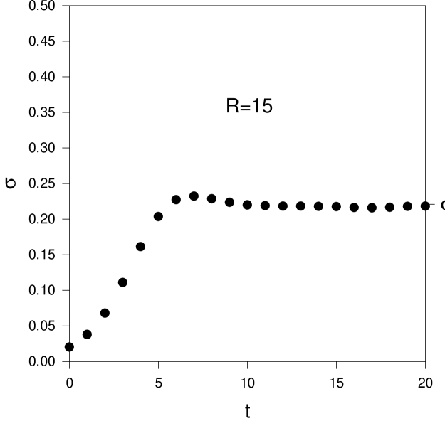
Figure 4: Typical plot of the $\sigma_{t}$ versus time, for $R=15$.

Condition (25) can be now used to find the dependence of $\sigma_{\infty}$ upon the radius $R$. As we already noted, $f(t,R)$ is asymptotically linear when $t\rightarrow\infty$, and the convergence is so fast that we can assume $f(t,R)=a(R)t+b(R)$ for large $t$. Using condition (25) we have

$$f(t,2R)=2f(t-1,R)=2a(R)t+b(R)-a(R),$$ (28)

which implies that $a(2R)=2a(R)$, i.e. $a(R)$ is proportional to $R$. This can be easily verified if we rewrite (27) as

$$a(R)\ln(1-n_{0})=\ln(1-\langle\sigma_{\infty}\rangle),$$ (29)

and plot the right hand side of the above equation versus $R$, as shown in Figure 5.

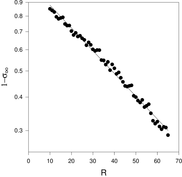
Figure 5: Plot of $\ln(1-\langle\sigma_{\infty}\rangle)$ as a function of $R$.

Of course, the slope $a(R)$ could also be measured directly from graphs of $f(t,R)$, and then plotted as a function of $R$. In both cases, $a(R)=\gamma R$, where $\gamma=0.89\pm 0.05$, and finally

$$\langle\sigma_{\infty}\rangle=1-(1-n_{0})^{\gamma R}.$$ (30)

As before, this expression is not very accurate if the radius $R$ is small (close to 1).

The value of $a(R)$, in a sense, provides us with a measure of a “speed” of convergence toward fixed point $n=1$, assuming we are sufficiently close to $n=1$. It does not carry, however, useful information about the early stage of the process, away from $n=1$ (all our previous derivations assume large $t$).

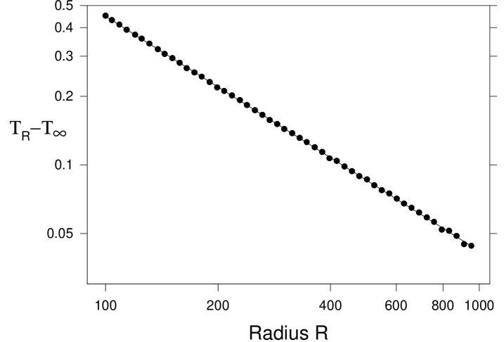
Figure 6: Asymptotic behavior of $T_{R}-T_{\infty}$ for large $R$.

Therefore, we will consider another quantity, often used in marketing, called the takeover time, and usually defined as the time required to go from $n=0.1$ to $n=0.9$. For an S-shaped curve, the inverse of its maximal slope carries a similar information as the takeover time, therefore we define

$$T_{R}=\left(\max_{t\in{\rm N}}\{(n_{t+1}-n_{t})\}\right)^{-1}.$$ (31)

Subsequently, $T_{R}$ will be used as a measure of the takeover time for a model with neighborhood radius $R$, and for simplicity we will just call it takeover time.

For $R=\infty$, the largest $n_{t+1}-n_{t}$ occurs at $t=5$, therefore

$$T_{\infty}=(n_{6}-n_{5})^{-1}=\left((1-n_{0})^{32}-(1-n_{0})^{64}\right)^{-1}$$ (32)

We used $n_{0}=0.02$, which yields $T_{\infty}=4.00915$.

We studied the asymptotic behavior of $T_{R}-T_{\infty}$ as $R$ tends to infinity (Figure 6). This log-log plot shows that $T_{R}$ tends to $T_{\infty}$ as $R^{-\alpha}$, where $\alpha=1.03\pm 0.01$. This exponent depends rather weakly on the initial density of adopters $n_{0}$. For example, if $n_{0}$ is two times smaller ($n_{0}=0.01$), $\alpha$ changes its value by approximately $2\%$, i.e. $\alpha=1.05\pm 0.01$. Note that in this case $T_{\infty}$ is different too, namely $T_{\infty}=4.01051$.

4 Conclusion and Remarks

We have studied a probabilistic cellular automata model for the spread of innovations. Our results emphasize the importance of the range of interaction between individuals, as the innovation propagates faster when the radius is larger. Increased connectivity between individuals reduces constraints on the exchange of information, and thus the growth rate increases. It should be pointed out that larger connectivity can be also achieved by increasing dimensionality of space. We performed some measurements of the takeover time in two and three dimensions (to be reported elsewhere), and as expected, the takeover time was found smaller when dimensionality increased. This is also consistent with the fact that, in general, in higher dimensions we are closer and closer to the mean-field approximation.

The behavior of local and global densities of adopters is an interesting feature of the model. While the global density of adopters always converges to $1$, the local density does not. It quickly reaches certain “equilibrium value” and stays constant after that (for infinite lattice only, since for a finite lattice both densities reach $1$ after a finite number of steps).

More sophisticated (and realistic) models can be constructed by relaxing some assumptions discussed in the introduction. For example, since every technology has a finite life span, we can allow adopters to go back to neutral state with a certain probability. Moreover, we can incorporate “reluctance” to adopt by assuming that the probability of adoption is not equal, but proportional to the local density of adopters. Such a generalized model exhibits a second order phase transition with a transition point strongly dependent on $R$. These results will be reported in details elsewhere.

References

- [1] Frank M. Bass. A new product growth for model consumer durables. Management Sciences, 15(5):215–227, 1969.
- [2] N. Boccara and K. Cheong. Automata network sir models for the spread of infectious diseases in populations of moving individuals. J. Phys. A: Math. Gen., 25:2447–2461, 1992.
- [3] N. Boccara and K. Cheong. Critical behaviour of a probabilistic automata network sis model for the spread of an infectious disease in a population of moving individuals. J.Phys. A: Math. Gen., 26:3707–3717, 1993.
- [4] N. Boccara, K. Cheong, and M. Oram. Probabilistic automata network epidemic model with births and deaths exhibiting cyclic behaviour. J. Phys. A: Math. Gen., 27:1585–1597, 1994.
- [5] T. Hagerstrand. The Propagation of Innovation Waves. Lund Studies in Geography. Gleerup, Lund, Sweden, 1952.
- [6] T. Hagerstrand. On Monte Carlo simulation of diffusion. Arch. Europ. Sociol., 6:43–67, 1965.
- [7] Kingsley E. Haynes, Vijay Mahajan, and Gerald M. White. Innovation diffusion: A deterministic model of space-time integration with physical analog. Socio-Econ. Plan. Sci., 11:25–29, 1977.
- [8] G. A. Hedlund. Endomorphisms and automorphisms of the shift dynamical system. Mathematical Systems Theory, 3(4):320–375, 1969.
- [9] Vijay Mahajan, Eitan Muller, and Frank M. Bass. New product diffusion models in marketing: A review and directions for research. Journal of Marketing, 54:1–26, 1990.
- [10] Vijay Mahajan and Robert A. Peterson. Models for Innovation Diffusion. Number 07-048 in Quantitative Applications in the Social Sciences. Sage Publications, Beverly Hills, 1985.
- [11] Everett M. Rogers. Diffusion of Innovations. The Free Press, New York, 1995.
- [12] Stephan Wolfram. Theory and applications of cellular automata. World Scientific, Singapore, 1986. ISBN 9971-50-124-4 pbk.