A model of macroevolution with a natural system size

Abstract

We describe a simple model of evolution which incorporates the branching and extinction of species lines, and also includes abiotic influences. A first principles approach is taken in which the probability for speciation and extinction are defined purely in terms of the fitness landscapes of each species. Numerical simulations show that the total diversity fluctuates around a natural system size $N_{\rm nat}$ which only weakly depends upon the number of connections per species. This is in agreement with known data for real multispecies communities. The numerical results are confirmed by approximate mean field analysis.

Keywords: Macroevolution, Bak-Sneppen model, speciation, extinction

The Bak-Sneppen model was introduced to illustrate the possible role of self-organised criticality in evolving ecosystems (Bak 1993, 1997). It is a toy model that describes every species by a single scalar quantity, relating to the expected time before that species evolves to a new form. Interactions in the ecosystem are incorporated by assuming that a species that evolves can alter the time taken for other species to evolve, such as those involved in predator-prey or host-parasite relationships. The model is said to be self-organised critical because it approaches a critical state without any apparent need for fine parameter tuning. Consequently, it predicts that extinction events of magnitude $\Delta E$ should occur with a frequency proportional to $(\Delta E)^{-\alpha}$, which is consistent with known paleobiological data (Solé 1996). Further evidence has come from analysis of the temporal distribution of extinctions, which exhibits “1/f noise”, also predicted by the model (Solé 1997a).

Other simple models of macroevolution have now been devised which also claim agreement with the paleobiological data (Peliti 1997). Some of these are believed to be self-organised critical (Solé 1997b), although others exhibit power law behaviour via different mechanisms (Roberts 1996, Newman 1997). All of these models have in common the assumption of a constant system size. This has been justified by assuming that each species occupies a single ecological niche, and that if a species is made extinct its niche is immediately filled by a similar, newly emerged species. The concept of an ecological niche refers to a set of conditions and interactions within the ecosystem that only a single species can satisfy. However, since the definition of a niche depends upon the other species, the total number of niches should be defined from within the system itself rather than being fixed to some arbitrary constant value for the benefit of computer simulation.

Models have been devised which are similar to the Bak-Sneppen model but allow the total number of species to vary in time. Kramer et al. introduced a model in which the species are placed onto a branching phylogenetic tree structure, where each species only interacts with its closest relatives (Kramer 1996). Depending upon the choice of a parameter, the tree either expands indefinitely or stops growing after a finite time. In the model of Wilke et al. the system refills after an extinction event at a rate according to a parameter $N_{\rm max}\,$, which is “the maximal number of species that can be sustained with the available resources” (Wilke 1997). However, since the resources are themselves biotic, we believe that any such $N_{\rm max}$ should be defined from within the system.

In this paper, we derive and study a version of the Bak-Sneppen model in which the probabilities for speciation and extinction are defined purely in terms of the individual species. Nonetheless, the total diversity fluctuates around a natural system size without the need for global control. In particular, there is no recourse to “ecological niches”. The rules of the model are based on careful considerations of the motion of species on their fitness landscapes. This is described in Sec. II, and the results of numerical simulations of the model are presented in Sec. III. Comparisons to real ecosystems are made in Sec. IV. Approximate analysis of the model is presented in Sec. V which supports and enhances the numerical work. Finally, we discuss our results in Sec. VI.

II Quantitative descriptions of macroevolution

To quantitatively describe an evolving ecosystem requires some general principle that applies equally to all species. A candidate for such a principle is to consider the relationship between an organism’s genotype and its fitness, which is some measure of the expected number of genes passed back into the species’ gene pool (Dawkins 1983). Each point in the multidimensional space of all possible genotypes can be assigned its own fitness value, forming a fitness landscape, as schematised in Fig. 1. The process of evolution can then be described as a walk over this landscape in the direction of increasing fitness. Rather than try to calculate the fitness for each genotype from first principles, clearly a hopeless task, Kauffman has assumed that the relationship is so complex that it can be well approximated by random variables (Kauffman 1993). This leads to the concept of rugged fitness landscapes, where “rugged” refers to the large variations in fitness that can result from small changes in genotype.

FIG. 1.: Schematic of a typical fitness landscape for a species labelled $i$, where for clarity the space of all possible genotypes has been compressed onto a single axis. The fitness scale is arbitrary. The barriers have heights of $f_{i1}$ and $f_{i2}$.

Models based on the Bak-Sneppen approach assume that each species moves on its own rugged fitness landscape, eventually becoming trapped in the region of a local maximum. If the landscape is fixed, then the species can only evolve by moving to a different maximum. Suppose that a species labelled $i$ is at a local maximum which is separated from nearby maxima by fitness barriers of heights $f_{ij}\,$, where $j=1,2,3,\ldots$ and the $f_{ij}$ are ordered such that $f_{ij}\leq f_{ij+1}$. Over time, fluctuations in the species’ fitness may bring it into the vicinity of one of its barriers, allowing it to crossover to a different maximum. This constitutes an evolutionary event in which the species changes from one typical genotype to another. For uncorrelated fluctuations, the expected time $\tau_{ij}$ to crossover a barrier of height $f_{ij}$ will be given by an Arrhenius equation of the form

$$\tau_{ij}\sim\exp(f_{ij}/f_{0})\>,$$ (1)

where the constant $f_{0}$ fixes the timescale and is analogous to temperature.

Since the landscape is rugged, a species that escapes from one maximum will soon become trapped by another, and will find itself surrounded by an entirely new set of barriers $f_{ij}$. In the limit $f_{0}\rightarrow 0$, (1) implies that it will always be the species $i$ with the smallest $f_{ij}$ in the system that evolves first, and that the other species will have moved no appreciable distance towards their own barriers by the time this occurs. Thus the ecosystem will consist of species that infrequently hop between maxima at a rate that depends upon the $f_{ij}\,$, but are otherwise essentially static. The evolution of species $i$ will alter the landscapes of all those species $k$ linked to it in the ecosystem, for instance via predator-prey or host-parasite relationships. Although each species $k$ will in general have to move on their new landscapes before finding a new maximum, it is a further approximation of the theory that this can be ignored and only the barriers $f_{kj}$ are affected.

The original Bak-Sneppen model is defined purely in terms of the smallest barriers $f_{i1}\,$, which are arranged on a lattice in such a way that interacting species occupy adjacent lattice sites. The evolutionary process described in the previous paragraphs then reduces to the dynamical interaction between adjacent $f_{i1}$. The system is static until the site with the smallest $f_{i1}$ evolves, when $f_{i1}$ and all of the $f_{k1}$ in adjacent sites $k$ are assigned new values. The system is again static until another site evolves, and so on. It has been shown that the essential system behaviour is insensitive to details such as the choice of probability distribution for the $f_{i1}$ (Bak 1993, Paczuski 1996). This robustness relates to the universality of the critical state, and is essential if such a simple model is to faithfully describe real ecosystems.

The Bak-Sneppen model can be enhanced by a more detailed consideration of the fitness landscapes and their interaction. Three features absent from the original model will be considered here, namely speciation, extinction and external noise. Each feature is described in general terms below before the new model is fully specified.

Speciation: Speciation occurs when two sub-populations reach a state of reproductive isolation and should be considered as separate species (Maynard-Smith 1993, Ridley 1993). For instance, two groups that are reunited after prolonged geographical isolation may have evolved so much in different directions that they are unable to produce viable offspring. Up until now, a species has been described as simply occupying a region of genotype space. More detailed analysis shows that a population forms a “cloud” of points of roughly equal fitness around the local maximum (Kauffman 1993). Normally the whole population crosses over the same barrier $f_{i1}$, but if $f_{i2}\approx f_{i1}$ then it is possible that part of the population will instead cross over the barrier $f_{i2}$. If this happens, the two subpopulations will move to different maxima and a speciation event will have occurred. A simple criterion for speciation is to say that species $i$ will branch into two subspecies if

$$f_{i2}-f_{i1}<\delta s$$ (2)

when it evolves to a new form, where $\delta s$ is a constant parameter. Further barriers could also be considered to incorporate the simultaneous splitting into three or more subspecies, but such events will be very rare and are ignored here.

Extinction: The system size would increase without limit if only speciation were allowed, so some mechanism is required by which a species can be made extinct and permanently removed from the system. The original Bak-Sneppen model does not distinguish between this form of extinction and pseudo-extinction, which is where a rapidly evolving species disappears from the fossil record if its intermediate forms are not recorded. What is required is some criterion for true extinction defined purely in terms of the individual species’ fitness landscapes, analogous to (2). It is not clear how this may be achieved. Instead, a heuristic approach is adopted here, which is to say that a species $k$ is made extinct if it is linked to the species with the minimum barrier, and has $f_{k1}$ greater than some threshold value. This proves to be the simplest choice for which the system size does not diverge.

External noise: A fitness landscape is ultimately a function of the species itself, the species with which it interacts, and any factors external to the ecosystem, so fluctuations in the inorganic environment can also cause the fitness barriers to change. Examples include local disturbances such as volcanic eruptions or the formation of a new river, to global events including meteor impacts and changes in the sea level. The interactions between species have already been incorporated into the model, but no allowance has yet been made for these abiotic factors. Continuing with the philosophy that changes in fitness can be approximated by random variables, external influences are assumed to alter the fitness landscapes by an amount $O(\delta g)$ per unit time, where $\delta g$ is a new parameter. More precisely, every species in the system will have their barriers altered by an amount

$$f_{ij}\rightarrow f_{ij}+\delta g_{ij}\>,$$ (3)

where the $\delta g_{ij}(t)$ are uniformly distributed on $[-\frac{\delta g}{2},\frac{\delta g}{2}]$ and uncorrelated in time. External effects will occur on a separate timescale to the evolutionary processes in (1), but for simplicity both timescales are fixed at the same constant rate in this model.

It remains to be decided how interacting species are linked together. The original Bak-Sneppen model placed the species on a regular crystalline lattice in which interacting species occupy adjacent sites, but this is not flexible enough to incorporate the addition of new species to the system and is of no use here. Real food webs have a much more involved structure, and if the full range of interactions is allowed rather than just links in the food chain, then it appears that a great many species interact at least weakly (Hall 1993, Caldarelli 1998). Trying to model this would only serve to draw attention away from the main motivation for the new model, which is to allow a variable system size. Instead, we adopt the mean field approach in which each species $i$ interacts with $K-1$ other species $k$ chosen at random from the system. The species $k$ are reselected at every time step.

The extended model can now be fully specified. The ecosystem consists of $N(t)$ species labelled by $i=1\ldots N(t)$. Each species occupies the region around a local maximum on a rugged fitness landscape, and is separated from nearby maxima by barriers of various heights $f_{ij}$. The larger barriers can be ignored since they will rarely contribute to the dynamics, but at least two must be retained if speciation is to be incorporated. Hence each species is defined by its two smallest barriers $f_{i1}$ and $f_{i2}$, which are uniformly distributed over the range [0,1] and then ordered so that $f_{i2}\geq f_{i1}$. The following steps (i)–(vi) are iterated for every time step.

(i) Evolution: The smallest $f_{i1}$ in the system is found and marked for evolution. It will move to a new maximum in step (vi).

(ii) Speciation: If the single species marked for evolution has $f_{i2}-f_{i1}<\delta s\,$, then a new species is introduced to the system with random barriers. $N\rightarrow N+1$.

(iii) Interaction: $K-1$ other species are chosen at random from the remaining $N-1$ in the system. They will be assigned new barriers in step (vi).

(iv) Extinction: If any the of the $K-1$ interacting species has $f_{i1}>1$, it is removed from the system. $N\rightarrow N-1$.

(v) External noise: Every barrier $f_{ij}$ in the system is transformed according to (3), and reordered if necessary.

(vi) New barriers: The species marked for evolution in step (i) and the $K-1$ interacting species from step (iii) are assigned new random barriers, ordered such that $f_{i2}\geq f_{i1}$.

With such specific definitions of general processes, it is obviously important to check that the model is robust to any arbitrary choices. To test this, the simulations have been repeated with various changes to the rules, and in no case was any qualitative deviation observed. For instance, different values for the extinction threshold in step (ii) give the same behaviour, even if the threshold value varies in time around a fixed mean. Both $\delta s$ and $\delta g$ were chosen from uniform, Gaussian and exponential distributions, again with no apparent change in behaviour. Since the model appears to be robust, further discussion will be restricted to the simple set of rules given in (i)–(vi). The threshold value for extinction was fixed at 1 to minimise the number of new parameters.

Before continuing, it should be pointed out that the algorithm presented in steps (i)–(vi) above is not exactly the same as that described in our previous exposition of this work (Head 1997). This earlier model assumed that all $K$ species “mutate” (evolve) at every time step, whereas it is of course just the species with the minimum barrier that evolves. The corrected model studied here behaves in much the same way as its previous incarnation, except that the number of species is now only weakly dependent on the connectivity $K$. This is in agreement with data for real multispecies communities, as discussed further in the next section.

III Results of numerical simulations

The quantity of interest is the total system size $N(t)$. This varies in a manner that depends upon the choice of values for the parameters $K$, $\delta s$ and $\delta g$, as described below.

$\bullet$ $\delta s=\delta g=0$: Steps (ii), (iv) and (v) never feature in the time evolution of the system and the larger barriers $f_{i2}$ are redundant. The $f_{i1}$ interact in the same way as the original Bak-Sneppen model, the only difference being that each $f_{i1}$ is the smaller of two uniform distributions on [0,1] and so is distributed according to $P(f_{i1})=2(1-f_{i1})$, $f_{i1}\in[0,1]$. Since the model is robust to the choice of probability distribution, this difference is not important. $N(t)$ remains fixed at its initial value.

$\bullet$ $K=1$: There are no interactions, and the species that evolves will always have $f_{i1}<1$ so extinction is impossible. $N(t)\rightarrow\infty$ if $\delta s>0$ or remains fixed if $\delta s=0$.

$\bullet$ $K>1$, $\delta s>0$ and $\delta g=0$: There is speciation but no extinction, $N(t)\rightarrow\infty$.

$\bullet$ $K>1$, $\delta s=0$ and $\delta g>0$: There is extinction but no speciation, $N(t)\rightarrow 0$.

$\bullet$ $K>1$, $\delta s>0$ and $\delta g>0$: $N(t)$ fluctuates around some constant value $N_{\rm nat}$ which is independent of the initial system size. An example is given in Fig. 2. Note that if $\delta g\gg\delta s$, $N_{\rm nat}$ is so small that statistical fluctuations will eventually send $N(t)\rightarrow 0$ and the simulation is over.

That $N_{\rm nat}$ should exist at all is by no means obvious, since $N(t)$ does not explicitly appear in the rules for speciation and extinction. It exists because of the external noise of order $\delta g$, which is just as likely to push two barriers apart as to bring them together and so does not affect the rate of speciation. However, the noise acts asymmetrically on barriers near the threshold for extinction, tending to push species over this threshold into the small tail corresponding to those species that will be made extinct when next selected. Since every species is subjected to external noise at every time step, the rate of extinction increases with $N$ whilst the rate of speciation remains roughly constant. A steady state will be found when these two rates balance. This qualitative reasoning is confirmed by the analysis in Sec. V.

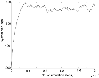
FIG. 2.: Plot of $N(t)$ against $t$ starting from a system with 200 species. $K=4$, $\delta s=0.008$ and $\delta g=0.02$.

IV Comparison to real multispecies communities

The parameters $\delta s$ and $\delta g$ are abstract quantities defined purely in terms of the model, so it is not possible to estimate their values for real ecosystems. Nonetheless it is intuitively reasonable to assume that speciation and extinction events are rare, and therefore both $\delta s$ and $\delta g$ should be small. The number of links per species $K-1$ has been measured for real communities, and according to some studies is independent of the system size (Hall 1993, Kauffman 1993). This is in agreement with numerical simulations of the model, which shows only a weak dependence on $K$ from the range $K=2$ to $K=16$, as given in Table I (at end of document). There is a small peak around $K\approx 4$, which also corresponds to the most common value of $K$ observed in nature. However, the data for real ecosystems is based on food webs whereas the Bak-Sneppen approach considers all direct interactions between species, so it is not clear how far this comparison can be taken.

Turning to consider global ecosystems, the fossil record for all marine organisms highlights the possibility of a statistical steady state throughout much of the Palaeozoic era. The total number of (families of) species fluctuates around a roughly constant value up until the mass extinction at the end of the Permian period, after which the system size increased beyond its earlier levels and is still increasing today (Benton 1995). It could be conjectured that the new species that emerged after the end-Permian extinction were on average either more likely to speciate, or less susceptible to external noise, or both, which should result in an increased system size according to the model. The data for continental organisms is less clear and if anything shows a continuing increase in diversity at varying rates.

The distribution of the magnitude of the change in $N$ per unit time is Poisson to first order, implying that the speciation and extinction events are uncorrelated for $N(t)\approx N_{\rm nat}$. However, the distribution is not precisely Poisson, which is presumably due to the tendency for $N$ to drift towards $N_{\rm nat}$ when $|\,N-N_{\rm nat}\,|$ is large. An example is presented in Fig. 3. That the distribution was not power law is disappointing, but perhaps unsurprising given that the interactions between species are randomised at every time step, making it difficult for the system to self-organise. It is possible that a spatially extended model might allow for correlations to build up towards a critical state and a power law to be recovered, but this must remain as speculation at present.

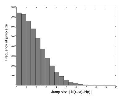
FIG. 3.: Distribution of the absolute change in system size per $\Delta t=10^{3}$ time steps for $K=2$, $\delta s=0.008$ and $\delta g=0.04$. $4\times 10^{4}$ points were sampled over 4 separate runs.

V Analytical derivation of $N_{\rm nat}$

It is possible to derive the dependence of $N_{\rm nat}$ on the parameters $K$, $\delta s$ and $\delta g$ by extending the mean field solution of the original Bak-Sneppen model (Flyvberg 1993). In theory this approach could give the exact solution, since the interacting species are selected at random in the new model and so it is mean field by definition. However, the increased dynamical complexity means that only the first order parameter dependence has be calculated.

Standard model with two barriers per species

The original solution was based on a single barrier per species. Before tackling speciation and extinction, it must first be shown how the mean field approach can be modified to handle pairs of barriers. Define $p(x,y)\,{\rm dx\,dy}$ to be the probability that a randomly selected species has one barrier in the range [ x,x+dx ) and the other in [ y,y+dy ). Note that this refers to the barriers $f_{ij}$ before ordering, so $x$ can be less that or greater than $y$. The probability for a species to have both barriers greater than $m=\min(x,y)$ is represented by $Q(x,y)$, which is related to $p(x,y)$ by

$$Q(x,y)=\int_{m}^{\infty}\!\!\int_{m}^{\infty}p(x^{\prime},y^{\prime})\,{\rm dx^{\prime}}{\rm dy^{\prime}}\>.$$ (4)

Since $p(x,y)=0$ for values of $x$ or $y$ outside the range [0,1], $Q(x,y)=1$ for $m\leq 0$ and $Q(x,y)=0$ for $m\geq 1$. The species with the smallest barrier can be any of the $N$ in the system, as long as all of the remaining $N-1$ species have larger barriers. Hence $p_{\rm min}(x,y)$, the probability distribution for the species with the smallest barrier, is given by

$$p_{\rm{min}}(x,y)=N\,p(x,y)\,Q^{N-1}(x,y)\>.$$ (5)

At each time step, $p(x,y)$ will change by an amount $\Delta p(x,y)$ which is given by the master equation

$$\Delta p(x,y)=-\frac{1}{N}p_{\rm{min}}(x,y)$$ (6)

$$\mbox{}-\frac{K-1}{N-1}\left(p(x,y)-\frac{1}{N}p_{\rm{min}}(x,y)\right)+\frac{K}{N}\>.$$ (7)

The first term on the right hand side of (7) accounts for the evolution of the species with the lowest barrier, the second for the new barriers assigned to the $K-1$ species with which it interacts, and the third term handles the $K$ new pairs of barriers. In the statistical steady state, $\Delta p=0$ and, using (5) and (7),

$$\frac{K}{N}-\frac{K-1}{N-1}p-\frac{N-K}{N-1}pQ^{N-1}=0\>.$$ (8)

The solution to (8) depends upon the behaviour of $Q^{N-1}$ as $N\rightarrow\infty$ (Flyvberg 1993). If $Q<1-O(1/N)$, then the term proportional to $Q^{N-1}$ vanishes and

$$p(x,y)=\frac{K}{K-1}+O\left(\frac{1}{N}\right)\>.$$ (9)

Conversely, if either $x$ or $y$ is so small that $p(x,y)=O(1/N)$, then the second term in (8) will be $O(1/N^{2})$ and $Q(x,y)=1+O(1/N)$, so

$$pQ^{N-1}=\frac{K}{N}+O\left(\frac{1}{N^{2}}\right)\>,$$ (10)

and hence from (5),

$$p_{\rm min}=K+O\left(\frac{1}{N}\right)\>.$$ (11)

Each solution applies in different regions of the $(x,y)$ plane, which, for large $N$, will be separated by sharply defined boundaries. These boundaries can be found by remembering that both $p$ and $p_{\rm min}$ are probability distributions and normalise to one. To first order in $1/N$, the full solutions are

$$p(x,y) \approx \left\{\begin{array}[]{ll}\frac{K}{K-1}&\mbox{$x$ and $y>1-\sqrt{\frac{K-1}{K}}$,}\\ 0&\mbox{otherwise,}\end{array}\right.$$ (14)

$$p_{\rm min}(x,y) \approx \left\{\begin{array}[]{ll}0&\mbox{$x$ and $y>1-\sqrt{\frac{K-1}{K}}$,}\\ K&\mbox{otherwise.}\end{array}\right.$$ (17)

Hence the species with the smallest barrier will always be found in the region where $p_{\rm min}(x,y)\approx K$, and its $K-1$ interacting species will always come from the region corresponding to $p(x,y)\approx K/(K-1)$.

Analysis for $\delta s$ and $\delta g$ non-zero but small

When either $\delta s>0$ or $\delta g>0$, the system size $N$ becomes a function of time and the algebra quickly becomes prohibitive. The simpler and more intuitive approach adopted here is to initially ignore speciation and extinction altogether and only incorporate the external noise of order $\delta g$. This leads to new solutions for $p(x,y)$ and $p_{\rm min}(x,y)$, from which the rates of speciation and extinction can be calculated even though they are no longer dynamically involved. The natural system size $N_{\rm nat}$ is then the value of $N$ for which the two rates balance. The analysis presented below assumes that $\delta g$ is small; large values of $\delta g$ and $\delta s$ are considered at the end of this section.

The effect of the external noise will be to perturb the solutions for $p$ and $p_{\rm min}$ given in (14) and (17), as schematised in Fig. 4. The master equation (7) must be modified in two ways. First, the external noise can cause barriers to move outside of the range [0,1], so the range of possible $x$ and $y$ must be extended. However, the barriers are still assigned values in the range [0,1] and the term for new barriers must be altered accordingly. Secondly, a term for the noise itself must be included. The new steady state equation is

$$\frac{K}{N}\,\theta(x)\,\theta(1\!-\!x)\,\theta(y)\,\theta(1\!-\!y)-\frac{K-1}{N-1}p$$ (18)

$$-\frac{N-K}{N-1}pQ^{N-1}+\frac{\delta g^{2}}{24}\bigtriangledown^{2}p=0\;\;,$$ (19)

$$\mbox{where}\;\;\;\theta(x)=\left\{\begin{array}[]{ll}1&\mbox{if $x\geq 0$,}\\ 0&\mbox{otherwise.}\end{array}\right.$$ (20)

The theta functions in the first term ensure that new barriers lie in the range [0,1]. The last term on the right hand side of (19) accounts for the external noise, where $\bigtriangledown^{2}$ is the Laplacian operator. A full derivation of this term is given in the appendix.

Rate of extinction: Each of the $K-1$ random neighbours will be made extinct if it has $x>1$ and $y>1$. Thus the rate of extinction $k_{E}$ is given by

$$k_{E}=(K-1)\int_{1}^{\infty}\!\!\int_{1}^{\infty}p(x,y)\,{\rm dx}\,{\rm dy}\>,$$ (21)

where the integral is over the region $p_{\rm E}$ in Fig. 4. Strictly speaking, the distribution in this equation should be $p-\frac{1}{N}p_{\rm min}$, but this distinction can be ignored for large $N$. When both barriers are large, $Q^{N-1}\sim 0$ and (19) can be simplified by the transformation

$$x\rightarrow x^{\prime} = \alpha(1-x)\;\;,$$ (22)

$$y\rightarrow y^{\prime} = \alpha(1-y)\;\;,$$ (23)

$$p\rightarrow p^{\prime} = \frac{K-1}{K}p\;\;,$$ (24)

$$\alpha^{2} = \frac{48(K-1)}{\delta g^{2}N}\;\;,$$ (25)

to give

$$2\bigtriangledown^{\prime 2}p^{\prime}(x^{\prime},y^{\prime})=p^{\prime}(x^{\prime},y^{\prime})-\theta(x^{\prime})\theta(y^{\prime})\>.$$ (26)

For either $x^{\prime}$ or $y^{\prime}$ negative, corresponding to $x>1$ or $y>1$, the second term on the right-hand side of (26) vanishes and the equation can be solved by separation of variables. Coupled with the boundary conditions $p^{\prime}(x^{\prime},y^{\prime})\rightarrow 0$ for $x^{\prime}\rightarrow-\infty$ or $y^{\prime}\rightarrow-\infty$, the solution is

$$p^{\prime}(x^{\prime},y^{\prime})=c\,e^{\frac{1}{2}(x^{\prime}+y^{\prime})}\>,$$ (27)

where $c$ is an arbitrary constant. Whatever the value of $c$, it must be independent of $K$ and $\delta g$ since these parameters do not appear in (26). Transforming back into the original variables gives the explicit parameter dependence,

$$p(x,y)=c\,\frac{K}{K-1}\,e^{-\frac{\alpha}{2}(x+y-2)}\;\;\;\mbox{for $x>1$ and $y>1$}\>.$$ (28)

Substituting this into (21) gives

$$k_{E}\propto\delta g^{2}N\frac{K}{K-1}\;\;.$$ (29)

Rate of speciation: It has not been possible to find a solution to (26) for $x<1$ and $y<1$. The variable separable solution does not behave correctly, and other methods tried have been fruitless. Instead, the $\delta g=0$ solution will be used as a first approximation. The rate of speciation $k_{S}$ will be proportional to the density of species with $|\,x-y\,|<\delta s$. Since only the species with the minimum barrier can speciate,

$$k_{S}=\int\!\!\int\theta(\delta s\!-\!|x\!-\!y|)\,p_{\rm min}(x,y)\,{\rm dx}\,{\rm dy}\>.$$ (30)

Substituting the explicit expression for $p_{\rm min}(x,y)$ from (17) into (30) gives

$$k_{S}\approx\delta s$$ (31)

for small $\delta s$. With $\delta g>0$, $p_{\rm min}(x,y)$ broadens and so the real rate of speciation will decrease for larger $\delta g$.

The value of $N_{\rm nat}$ can now be found up to parameter dependence. The rates of speciation and extinction balance when $k_{E}=k_{S}$, and therefore

$$N_{\rm nat}\propto\frac{\delta s}{\delta g^{2}}\>.$$ (32)

This implies that $N_{\rm nat}\delta g^{2}/\delta s$ should be roughly constant. This quantity has been calculated from the numerical simulations and is shown in Table III. The agreement is good for variations in $\delta g$, but less so for $K$ and $\delta s$. This most probably reflects the first order approximation used in deriving $k_{S}$ in (31).

FIG. 4.: Graphical representation of the effects of external noise on the distribution of barriers $p(x,y)$. Denser shading corresponds to higher values of $p(x,y)$. The region labelled “$p_{\rm E}$” refers to species with both $x>1$ and $y>1$, which are liable to extinction.

Either $\delta s$ or $\delta g$ large

For the sake of completeness, the equivalent expression to (32) will now be derived for large $\delta s$ or $\delta g$, although such values bear no relevance to actual systems. If $\delta s$ is large but $\delta g$ small, the system size rapidly increases and with it the expected time a species will move under the influence of external noise before being assigned new barriers. Similarly, if both $\delta s$ and $\delta g$ are large, then the system behaviour is also dominated by the external noise. This is called the noise dominated regime. If $\delta s$ is small but $\delta g$ large, $N_{\rm nat}$ becomes so low that fluctuations will eventually drive every species in the system to extinction.

In the noise dominated regime, $p(x,y)$ will no longer be just a small perturbation around the original solution but will extend to large positive and negative values in both the $x$ and $y$ directions. Since the external noise is isotropic, $p(x,y)$ will be symmetric about the $x$ and $y$ axes and at most 1 in 4 species have both barriers in the $p_{\em E}$ region. Hence the rate of extinction will approach its upper bound value of

$$k_{E}\approx\frac{K-1}{4}\>.$$ (33)

When a barrier is assigned a new value in the range [0,1], it undergoes an unbiased random walk until it is again assigned a new value and brought back to near the origin. The average number of steps in this walk will be $O(N/K)$ and, since the average step size is $O(\delta g)$, an analogy with a one-dimensional random walker implies that the total distance travelled will be $O(\delta g\sqrt{N/K})$ (Papoulis 1991). This gives the width of the barrier distribution in both the $x$ and $y$ directions. The number of species in the infinite strip $|\,x-y\,|<\delta s$ is inversely proportional to the width of $p(x,y)$, so the rate of speciation is now given by

$$k_{S}\sim\frac{\delta s}{\delta g}\sqrt{\frac{K}{N}}\>.$$ (34)

As $N$ increases, the rate of extinction will remain roughly constant but now the rate of speciation will decrease until a balance is found at $N=N_{\rm nat}$. From (33) and (34), the corresponding value of $N$ is

$$N_{\rm nat}\propto\frac{1}{K}\left(\frac{\delta s}{\delta g}\right)^{2}\;\;.$$ (35)

A convenient way to display the crossover in behaviour from small $\delta g$ to the noise dominated regime is to consider $N_{\rm nat}$ as a function of $\delta=\delta s=\delta g$. According to (32) and (35), this should change from $N\sim\delta^{-1}$ for small $\delta$ to $N\sim\delta^{0}$ for large $\delta$. Numerical results in support of this prediction are presented in Fig. 5.

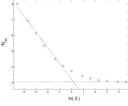
FIG. 5.: Plot of $N_{\rm nat}$ versus $\delta=\delta s=\delta g$ for $K=2$, demonstrating the crossover to the noise dominated regime. Each point corresponds to a single run of $10^{6}$ time steps. The dashed lines have slopes of $-1$ and 0.

VI Discussion

In summary, we have postulated one possible way in which models of macroevolution based on the Bak-Sneppen approach can be extended to incorporate speciation, extinction and abiotic influences. The speciation and extinction mechanisms are defined purely in terms of each individual species’ fitness landscape, irrespective of the total number of species in the system. Nonetheless, the total diversity fluctuates around a constant value $N_{\rm nat}$, which was termed the natural system size to stress that it was not arbitrarily chosen.

Although the proposed mechanism for speciation, ie. a population simultaneously crossing two different fitness barriers, seems appealing, the extinction mechanism is far more heuristic and somewhat unsatisfactory. A better model might focus on trying to find a more plausible means of extinction, defined in terms of the fitness landscapes. For instance, the species chosen for evolution might be made extinct if its fitness barrier is below some threshold value. It may also be possible to place the model on a web structure, and allow the connections themselves to be subject to alteration whenever a species evolves to a new form.

The value of $N_{\rm nat}$ was found to be only weakly dependent upon the average number of connections per species in the system, in agreement with known data. This leads us to hope that simple models such as ours may be able to reproduce the essential behaviour of real ecosystems. More realistic models consider the full fitness landscapes rather than just the barriers, but the increased complexity limits the system sizes that can be simulated (Kauffman 1993). A practical step forward might be to reduce known biological principles to simple rules that may be applied to global ecosystems.

References

Bak P. and Sneppen K. 1993 “Punctuated equilibria and criticality in a simple model of evolution” Phys. Rev. Lett. 71 4083-4086

Bak P. 1997 “How nature works:The science of self-organized criticality” Oxford University Press

Benton M. J. 1995 “Diversification and extinction in the history of life” Science 268 52-58

Caldarelli G., Higgs P. G. and McKane A. J. 1998 “Modelling coevolution in multispecies communities” preprint adap-org/9801003

Dawkins R. 1982 “The extended phenotype” Oxford University Press

Flyvberg H., Sneppen K. and Bak P. 1993 “Mean-field theory for a simple model of evolution” Phys. Rev. Lett. 71 4087-4090

Hall S. J. and Raffaelli D. G. 1993 “Food webs - Theory and reality” Adv. Ecol. Res. 24 187-239

Head D. A. and Rodgers G. J. 1997 “Speciation and extinction in a simple model of evolution” Phys. Rev. E 55 3312-3319

Kauffman S. A. 1993 “The Origins of Order” Oxford University Press

Kramer M. Vandewalle N. and Ausloos M. 1996 “Speciations and extinctions in a self-organising critical model of tree-like evolution” J. Phys. I (France) 6 599-606

Maynard-Smith J. 1993 “The theory of evolution” Cambridge University Press

Newman M. E. J. 1997 “A model of mass extinction” J. Theor. Biol. 189 235-252

Paczuski M. Maslov S. and Bak P. 1996 “Avalanche dynamics in evolution, growth and depinning models” Phys. Rev. E 53 414-443

Papoulis A. 1991 “Probability, random variables and stochastic processes” McGraw-Hill

Peliti L. 1997 “An introduction to the statistical theory of Darwinian evolution” preprint cond-mat/9712027

Ridley M. 1993 “Evolution” Blackwell Scientific Publications

Roberts B. W. and Newman M. E. J. 1996 “A model for evolution and extinction” J. Theor. Biol. 180 39-54

Solé R. V. and Manrubia S. C. 1996 “Extinction and self-organised criticality in a model of large-scale evolution” Phys. Rev. E 54 R42-45

Solé R. V., Manrubia S. C., Benton M. and Bak P. 1997a “Self-similarity of extinction statistics in the fossil record” Nature 388 764-767

Solé R. V. and Manrubia S. C. 1997b “Criticality and unpredictability in macroevolution” Phys. Rev. E 55 4500-4507

Wilke C. and Martinetz T. 1997 “Simple model of evolution with variable system size” Phys. Rev. E 56 7128-7131

Appendix

In this appendix, the term for external noise that appears in (19) is derived. Assuming that $\delta g$ is small, noise effects alone will result in $p(x,y)$ taking the mean value of the surrounding square with sides $\delta g$, that is

$$\Delta_{\rm noise}\,p(x,y)=-p(x,y)$$ (36)

$$\mbox{}+\frac{1}{\delta g^{2}}\int_{x-\delta g/2}^{x+\delta g/2}\int_{y-\delta g/2}^{y+\delta g/2}p(u,v)\,{\rm du}\,{\rm dv}\>.$$ (37)

Since $\delta g$ is small, $p(x,y)$ can be expanded according to Taylor’s theorem as

$$p(x+\delta x,y+\delta y)=p(x,y)+\delta x\frac{\partial p}{\partial x}\,+\,\delta y\frac{\partial p}{\partial y}$$ (38)

$$\mbox{}\,+\,\frac{\delta x^{2}}{2!}\frac{\partial^{2}p}{\partial x^{2}}\,+\,\delta x\delta y\frac{\partial^{2}p}{\partial x\partial y}\,+\,\frac{\delta y^{2}}{2!}\frac{\partial^{2}p}{\partial y^{2}}+\ldots$$ (39)

On substituting this into (37), the terms in $\delta x$, $\delta y$ and $\delta x\delta y$ integrate to zero, leaving just the leading-order term

$$\Delta_{\rm noise}\,p(x,y)=\frac{\delta g^{2}}{24}\bigtriangledown^{2}p(x,y)+O(\delta g^{3})\>,$$ (40)

where $\bigtriangledown^{2}$ is the two-dimensional Laplacian operator,

$$\bigtriangledown^{2}\equiv\frac{\partial^{2}}{\partial x^{2}}+\frac{\partial^{2}}{\partial y^{2}}\;\;.$$ (41)

The new term $\Delta_{\rm noise}\,p(x,y)$ is added to (7), the expression for $\Delta p(x,y)$ for when $\delta g=0$, to give the total change in $p(x,y)$ at every timestep for $\delta g>0$. Setting this to zero then gives the new steady state equation (19).

K	$\delta s$	$\delta g$	Numerical $N_{\rm nat}$	$N_{\rm nat}\delta g^{2}/\delta s$
2	0.008	0.02	625(19)	31(1)
4	0.008	0.02	741(21)	37(1)
6	0.008	0.02	717(22)	36(1)
8	0.008	0.02	699(19)	35(1)
16	0.008	0.02	615(17)	31(1)
4	0.008	0.02	741(21)	37(1)
4	0.008	0.04	187(12)	37(2)
4	0.008	0.08	50(6)	40(5)
4	0.004	0.02	418(20)	42(2)
4	0.008	0.02	741(21)	37(1)
4	0.016	0.02	1257(25)	31(1)

TABLE I.: Observed values of the natural system size $N_{\rm nat}$ for different $K$, $\delta s$ and $\delta g$. The standard deviation of the fluctuations are given in brackets, which also serve as rough error bars. The data has been averaged over at least three separate rune of $10^{6}-10^{7}$ timesteps each. Note that the line for $K=4$, $\delta s=0.008$ and $\delta g=0.02$ appears three times to allow for easier comparison.