Physical Complexity of Symbolic Sequences

Abstract

A practical measure for the complexity of sequences of symbols (“strings”) is introduced that is rooted in automata theory but avoids the problems of Kolmogorov-Chaitin complexity. This physical complexity can be estimated for ensembles of sequences, for which it reverts to the difference between the maximal entropy of the ensemble and the actual entropy given the specific environment within which the sequence is to be interpreted. Thus, the physical complexity measures the amount of information about the environment that is coded in the sequence, and is conditional on such an environment. In practice, an estimate of the complexity of a string can be obtained by counting the number of loci per string that are fixed in the ensemble, while the volatile positions represent, again with respect to the environment, randomness. We apply this measure to tRNA sequence data.

1 Introduction

The study of “complex systems”, or more generally the science of “complexity”, has enjoyed tremendous growth in the last decade, despite the fact that complexity itself is only vaguely defined, and many alternatives have been proposed over the years (see, e.g., [1, 2, 3, 4, 5]). In this paper we focus on the complexity of symbolic sequences (mostly binary), as most systems whose complexity we would like to estimate can be reduced to them.

In searching for an adequate measure for the complexity of binary strings, two limiting cases must be considered: the regular strings (such as a sequence of only zeros) and the random ones. A good measure of physical complexity is expected to yield a vanishing complexity for both cases, while the “intermediate” strings that appear to encode a lot of information are thought to be complex. Surprisingly, such a measure has been difficult to define consistently. Here we propose a measure of physical complexity that has the above-mentioned property, but can consistently be defined within automata theory and information theory. Contrary to the intuition that the regularity of a string is in any way connected to its complexity (as in Kolmogorov-Chaitin theory), we will argue here that such a classification is, in the absence of an environment within which the string is to be interpreted, quite meaningless. Rather, a “regular” string given by a uniform sequence can be made to represent anything (e.g., all of Shakespeare’s “Hamlet”) if the coding is complicated enough. In such a case, the coding rules represent part of the sequence’s environment. Indeed, we propose that the complexity of a string should, rather than focusing on its regularity, be determined by analyzing its correlation with a physical environment. Similarly, “randomness” is a meaningless concept without reference to this environment. In general, we will find that a sequence can be random with respect to one environment while perfectly “meaningful” with respect to another. In all cases, however, estimating the complexity requires an ensemble of sequences and an environment with which it is correlated.

In the next section we briefly review Kolmogorov-Chaitin complexity to establish our notation and point out its well-known shortcomings as a measure of physical complexity. Physical complexity is introduced in Section 3, and its relation to notions from conventional (Shannon) information theory is pointed out in Section 4. Practical considerations for the estimation of complexities are presented in the subsequent section. A real-life example is offered in Section 6, by giving an estimate of the complexity of a tRNA sequence. Section 7 contains some speculations about the evolution of complexity in simple living systems.

2 Kolmogorov Complexity

Kolmogorov-Chaitin (KC) complexity [1, 2] is rooted in automata theory [6], and provides a measure for the regularity of a symbolic string. Roughly, a string is said to be “regular” if the algorithm necessary to produce it on a universal (Turing) automaton is shorter (with length measured in bits) than the string itself. A simple example is a bit string with a repetitive pattern, such as 1010101010… The minimal “program” enabling a Turing automaton to write this string only requires the pattern 10, the length of the string, and “repeat, write” instructions. A less obvious example is the binary equivalent of, say, the first one hundred digits of $\pi$. While random prima facie, a succinct algorithm for a Turing machine can be written; as a consequence such a string is classified as regular. Technically, the KC-complexity of a string $s$ is defined (in the limit of long strings) as the length (in bits) of the shortest program $p$ producing $s$ when run on universal Turing machine $T$:

$$K(s)={\rm min}\,\left\{|p|:\,\,s=C_{T}(p)\right\}\;,$$ (1)

where $|p|$ denotes the length of the program in bits and $C_{T}(p)$ is the result of running program $p$ on Turing machine $T$. While KC-complexity is only defined modulo the number of prefix instructions (to be added to the program) necessary to simulate any other computer, it becomes exact in the limit of infinite strings.

A simple consequence of (1) is that algorithmically regular strings have vanishing KC-complexity in the limit of infinite strings, while “random” strings (such as binary strings obtained from a coin-flip procedure) are assigned maximum KC-complexity, i.e., for a random string $r$:

$$K(r)\approx|r|\;.$$ (2)

Physically, and intuitively, this is unsatisfactory, and requires us to rethink the very definition of “random” in a physical world. Our intuition demands that the complexity of a random string ought to be zero, as it is somehow “empty”. Furthermore, it has been known for some time that randomness, from an automata-theoretic point of view, must be undecidable, owing to Gödel’s undecidability theorem applied to the halting problem: No halting computation can possibly determine that a string is random, simply because such a computation would render the string non-random [7]. In Eq. (2), this problem is circumvented by allowing a random string to be computed by a Turing machine if it is included verbatim on the program tape. Besides redefining the concept of randomness, such a definition implies the (physically unsatisfactory) property that random strings are maximally complex. Below, we show how all these problems can be averted by insisting that physical Turing machines never operate without context, i.e., without an environment.

3 Physical Complexity

In order to define physical complexity, we first need to recall the notion of “conditional complexity” defined earlier by Kolmogorov. The idea implements precisely what we have called for earlier: that the determination of the complexity of a sequence should depend—be conditional on—the environment that the sequence is interpreted within. The traditional Kolmogorov complexity, however, is only conditional on the implicit rules of mathematics, and nothing else. These rules are necessary to interpret the program on the tape, but are usually not sufficient, as we shall see below. Instead, let us imagine a Turing machine that takes an infinite tape $e$ as input (which represent its physical environment) and that includes the particular rules of mathematics of this “world”. Without such a tape, this Turing machine is incapable of computing anything, except for writing to the output what it reads in the input. Thus, in the absence of the infinite tape $e$ all strings have maximal complexity. In other words, the aforementioned string that represents $\pi$ also has maximal complexity if it is unconditional on any rules (in contrast with the KC construction).

In this spirit, we can define the conditional complexity $K(s|u)$ [1, 8] as the length of the smallest program that computes $s$ from $e$:

$$K(s|e)=\min\ \{|p|:s=C_{T}(p,e)\}\;,$$ (3)

where $C_{T}(p,e)$ denotes the result of running program $p$ on Turing machine $T$ given input string $e$. This is not yet a physical complexity. Rather, the smallest program that computes $s$ from $e$, in the limit of infinite strings, will contain bits that are entirely unrelated to $e$, since, if they were not, they could be obtained from $e$ with a program of size tending to zero. Thus, $K(s|e)$ represents those bits in $s$ that are random with respect to $e$. If $e$ were to represent the usual rules of mathematics only, the complexity of $\pi$ (for example) conditional on $e$ reduces to the KC complexity of $\pi$, i.e., zero.

The physical complexity can now be defined as the number of bits that are meaningful in $s$ (that can be obtained from $e$ with a program of vanishing size) and is given by the “mutual complexity” [1, 8]

$$K(s:e)=K_{0}(s)-K(s|e)\;.$$ (4)

Here, we have introduced the unconditional complexity $K_{0}(s)$, i.e., the complexity given an empty input tape $e\equiv\emptyset$. This is different from the Kolmogorov complexity $K(s)$ described above because, in Kolmogorov’s construction, the rules of mathematics were given to the automaton. As argued for above, every string is random if no $e$ is specified, as non-randomness can only exist with respect to a specific world, or environment. Thus, $K_{0}(s)$ is always maximal, given by the length of $s$:

$$K_{0}(s)=|s|\;.$$ (5)

Consequently, as Eq. (4) represents the length of the string minus those bits that can not be obtained from $e$, $K(s:e)$ represents the number of bits that can be obtained, by a computation with vanishing program size, from $e$. Thus, this represents the physical complexity of $s$. Let us investigate the connection of these results to standard Shannon information theory [9].

4 Physical Complexity and Information Theory

In fact, a moment’s reflection reveals that $K(s:e)$, the complexity of string $s$ given a description of the environment $e$, is not practical, meaning that it can not, in general, be determined by inspection. In other words, it is impossible to determine which, and how many, of the bits of string $s$ correspond to information about $e$. The reason is that in general, we are unaware of the coding used to code information about $e$ in $s$, and as a consequence coding and non-coding bits look entirely alike. However, it is possible to determine coding versus non-coding bits if we are given multiple copies of a symbolic sequence that have adapted independently to the environment within which it is to be interpreted, or more generally, if a statistical ensemble of strings is available to us. In that case, coding bits are revealed by non-uniform probability distributions across the ensemble (“conserved sites”), whereas random bits sport uniform distributions (“volatile sites”). The determination of complexity then becomes an exercise in information theory. Indeed, the link between automata theory and information theory has been pointed out quite early, as it was realized [10] that the average complexity $\langle K\rangle$, in the limit of infinitely long strings tends to the entropy of the ensemble of strings $S$

$$\langle K(s)\rangle_{S}=\sum_{s}p(s)K(s)\approx H(S)=-\sum_{s}p(s)\log p(s)\;,$$ (6)

where string $s$ appears in the ensemble $S$ with probability $p(s)$. Note that this is consistent with our determination that $K(s)$, in the absence of an environment $e$, must equal the string’s length. Indeed, if nothing is known about the environment that the strings $s$ pertain to, the probability distribution $p(s)$ must be uniform (principle of insufficient reason). As a consequence (if logarithms are taken to base 2), $H(S)=|s|$, where $|...|$ as before denotes the size of a string. On the other hand, if an environment $e$ is given we have some information about the system, and the probability distribution is non-uniform. Indeed, it can be shown that for every probability distribution $p(s|e)$ to find $s$ given $e$, we have

$$H(S|e)\leq H(S)=|s|\;.$$ (7)

as a result of the concavity of Shannon entropy. The difference between the maximal entropy $H(S)=|s|$ and $H(S|e)$, according to the construction outlined above, should then represent the average number of bits in strings $s$ taken from the ensemble $S$ that can be obtained by zero-length universal programs from $e$:

$$\langle K(s:e)\rangle_{S}=\sum_{s}p(s)\,K(s:e)\approx H(S)-H(S|e)\equiv I(S:e)\;.$$ (8)

In Eq. (8), we used the usual definition of information theory that the difference between the “marginal” entropy $H(S)$ and the entropy of $S$ given $e$, $H(S|e)$, is just the information about $e$ contained in the ensemble $S$. Note that strictly speaking, $I(S:e)$ is not an information. Rather, an information is obtained only if $I(S:e)$ is averaged over possible occurrences of $e$ in an ensemble $E$

$$I(S:E)=\sum_{e}p(e)\,I(S:e)\;.$$ (9)

Despite this, we shall in the following continue to refer to $I(S:e)$ as the information about $e$ stored in $S$. We now ask the question whether the physical complexity $I(S:e)$ is a measurable quantity.

5 Estimating Entropies in Finite Ensembles

In general, the entropy

$$H(S|e)=-\sum_{s}p(s|e)\log p(s|e)$$ (10)

can be estimated by sampling the probability distribution $p(s|e)$. In a population of $N$ strings in environment $e$, the quantity $n(s)/N$ where $n(s)$ denotes the number of strings of type $s$, approximates $p(s|e)$ arbitrarily well as $N\to\infty$. However, if the number of different strings is very large as is typically the case for symbolic strings (in particular genetic ones), the sampling error incurred from a population that is not exponentially large can be overwhelming. Indeed, it is known [12] that for symbolic strings that can take on $M$ states, the sampling error in the entropy, to first order in $1/N$, is

$$\Delta H=\frac{M-1}{2N}\;,$$ (11)

if we agree to take logarithms to the base of the alphabet-size. Thus, for strings of length $\ell$ constructed from an alphabet of size $D$ only populations of the order $N\simeq D^{\ell}$ will ensure that the finite-size error of the entropy is of order 1. In most practical cases, such ensembles are unrealistic. Still, we may attempt to estimate the entropy by summing the per-site entropies of the string. Random sites, identified by a nearly uniform probability distribution, contribute positively to the entropy whereas non-random sites (which have strongly peaked distributions) contribute very little. Thus,

$$H(S|e)\approx\sum_{i}H(x_{i}|e)\;.$$ (12)

Using this estimate, however, introduces a systematic error which is due to the fact that the particular code used to encode the sequence may not be optimal. Let us consider as an example a sequence of length two with positions $a$ and $b$, or more generally a sequence $s$ arbitrarily partitioned into subsequences $a$ and $b$: $s=ab$ (see Fig. 1.)

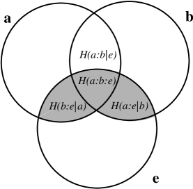
Figure 1: Entropy diagram for a string $s=ab$ (with subsequences $a$ and $b$) in environment $e$, with notations. The shaded region is the complexity $I(ab:e)$. The areas that are not filled in in this diagram are irrelevant for the determination of complexity.

The physical complexity in an environment $e$ is, according to Eq. (8), given by

$$I(S:e)=H(ab)-H(ab|e)\;,$$ (13)

i.e., the entropy of string $s$ irrespective of any environment (or, equivalently, averaged over all possible environments) minus the entropy given the particular environment (see shaded region in Fig. 1). This can be rewritten as

$$I(S:e) = H(a)+H(b)-H(a|e)-H(b|e)-H(a:b:e)$$ (14)

$$= |s|-\sum_{i}H(x_{i}|e)-H(a:b:e)\;,$$ (15)

where we introduced the short hand $|s|=H(a)+H(b)$, i.e., the sum of the unconditional per-site entropies is just the length of the sequence, and $\sum_{i}H(x_{i}|e)$ is the sum of the per-site conditional entropies. It is the latter which can be measured in actual populations. Approximating the physical complexity by

$$C\simeq|s|-\sum_{i}H(x_{i}|e)$$ (16)

[i.e., replacing the true entropy as in Eq. (12)] thus misses a piece $H(a:b:e)$, the center of the diagram in Fig. 1. Now, for perfect codes $H(a:b:e)$ actually vanishes, because all bits of $s$ must be independent of each other when ignoring the environment (i.e., the particular coding rules) $e$. This implies that the information is optimally stored in $s$ (it is perfectly compressed), which is the case when taking the average of mutual KC complexity [see Eq. (8)], as the limit of perfect codes is always implied there. In physical ensembles, the error remains, and can only be minimized by reducing the influence of correlations in $\sum_{i}H(x_{i}|e)$. How this can be done approximately will be shown below using tRNA as an example. Note that $H(a:b:e)$ can be positive as well as negative, implying that $C$ is neither a lower nor an upper bound on the complexity.

6 Complexity of Genomes

As an example, let us find an approximation for the complexity of biological sequences. Our purpose here is to outline the practical aspects of such a determination based on the complexity measure proposed, rather than an examination of the feasibility of this method with current technology. Consider for the purpose of illustration the molecule tRNA, which consists out of 76 nucleotides that contort into the well-known clover-leaf secondary structure (see Fig. 2), and whose tertiary structure is essential for the translation of codons to amino acids. If the complexity of this molecule is represented by the genomic complexity of its sequence $s_{\rm RNA}$, then the complexity of tRNA can be obtained by identifying the shortest description of the random part of $s_{\rm RNA}$ (as this represents $K(S|u)$) and subtracting it from the length of the molecule. Replacing $K$ by its average, the physical complexity is then the length of the string minus the remaining randomness according to Eq. (16), and should represent the essence which generates the RNA’s function.

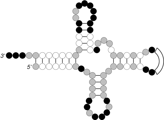
Figure 2: Secondary structure of tRNA with 76 common positions, of which 52 are independent and thus useful in the determination of the sequence complexity. Fixed positions are black, moderately diverged ones are grey, and highly volatile ones are colored white (from [13].)

For tRNA from a given species, access to an ensemble of sequences allows a classification of each position according to its volatility. For Bacillus subtilis for example, we can use a sample of 32 aligned (structurally similar) sequences to determine whether nucleotide positions are volatile (white in Fig. 1), moderately diverged (grey) or fixed (black) [13]. Counting the black (and to some extent the grey) sites should approximate the complexity of the sequence. But is this code optimal for tRNA, or is there a substantial piece of the type $H(a:b:e)$ mentioned above? Such a piece represents correlations between sites in the string which are also correlated to the environment, i.e., they are important for function. In fact, all those sites that form Watson-Crick pairs in the secondary structure of the molecule (and which show some variation) contribute to such an error, as their contribution to the entropy in Eq. (16) will be double-counted.

An example of this is given in Fig. 3, which depicts the entropy diagram of positions 27 and 31 in the sequence in Fig. 2 (nucleotide 27 is paired with nucleotide 31 in the anticodon stem.)

Figure 3: Entropies for nucleotide positions 27 and 31 in the anticodon stem. The error in the entropy of the pair (27,31) contributing to the error in the complexity $I(S:e)$ is given by the center of the diagram. Not counting one of the two in the sum of per-site entropies eliminates this error.

Counting paired positions only once (the per-site entropy of base-paired positions are usually equal) and ignoring the anti-codon leaves 52 “reference positions”. Using the sequence data to calculate $H(x_{i})$ for each of the 52 positions reveals that the sum of their entropies is approximately 29 nucleotides (58 bits.) The complexity estimate for this sequence is thus (ignoring the anti-codon in $\ell$ also)

$$C=\ell-\sum_{i}\!{}^{\prime}\,H(x_{i}|e)=73-29=44\ {\rm nucleotides}\;,$$ (17)

where $\sum^{\prime}$ denotes the sum over reference positions only. Naturally, only correlations due to base-pairing are eliminated in this manner. Correlations due to other epistatic effects remain. Note also that the estimate of the entropy $H\approx 29$ is subject to the finite sample error (11), and is thus only accurate to 5%.

7 Evolution of Complexity

We can also extend our horizon and ask whether the evolution of physical complexity displays the trend of evolution toward higher complexity that seems evident in living systems (see, e.g., [15]). While we have an intuitive feeling that such an evolution towards higher complexity is responsible for the emergence of higher and higher organisms throughout time, such a statement must be questionable as long as there is no unambiguous measure of complexity.

Evolution of complexity can be observed explicitly in artificial living systems [16] which involve segments of (computer)-code self-replicating in a noisy environment replete with information. In such systems, an information landscape is specified by the user, and a population of self-replicating computer programs is allowed to adapt to it without external interference. More precisely, the “accidental” discovery (via random mutations) of a sequence that benefits the string is “frozen” in the genome owing to the higher replication rate of its bearer. The replication of each string is effected by executing its code on a virtual computer. As such, these strings are analogous to catalytically active RNA sequences that serve as the templates of their own reproduction.

The information-bearing sections of the code become apparent in equilibrated populations of self-replicating code as they are fixed, while the volatile positions provide for genomic diversity without storage of information. Again, the determination of volatility of a site is only possible statistically, i.e., by examining ensembles of members of the same “species”. Adaptive events (in which the replication rate increases) decrease the number of volatile instructions if the sequence length stays constant, while a size increase without commensurate acquisition of information increases that number [16]. Consequently, physical complexity (measured sufficiently far away from an adaptive event in order to allow equilibration) only increases in evolution.

According to the above arguments, the number of non-volatile instructions in a code within a given environment represents an estimate of the physical complexity of a particular species of string. Placed in a different environment, the strings are meaningless; they will not replicate anywhere except for the specific (real or virtual) world they have evolved in. Furthermore, in a different world all (previously) fixed positions will, under the influence of noise, revert to volatile ones. Thus, as emphasized throughout this paper, the information content, or complexity, of a genomic string by itself (without referring to an environment) is a meaningless concept. In artificial living systems, the increase of physical complexity, which coincides with increasing acquisition and storage of information, can be monitored directly, and illustrates the usefulness of this measure. Note that this process of acquisition of information constitutes, in the language of thermodynamics, to the operation of a natural Maxwell-demon: the population performs random measurements on its environment, and stores those “results” that decrease the entropy, but rejects all others. Thus, the process can be likened to a semi-permeable “membrane” for information, and the physical complexity increases as a function of evolutionary time (given a fixed environment) as the strings store more and more information about that environment. Naturally, a change in environment (catastrophic or otherwise) generally leads to a reduction in complexity. Such experiments suggest that physical complexity is indeed the “quantity that increases when self-organizing systems organize themselves” [17].

This work was supported by the National Science Foundation under Grant No. PHY-9723972. We are indebted to Tom Schneider for pointing out Ref. [12], and to C. Ofria and W.H. Zurek for discussions.

References

- [1] A.N. Kolmogorov, Three approaches to the definition of the concept “quantity of information”, Problems Inform. Transmission 1 (1965) 1-7; Combinatorial foundations of information theory and the calculus of probabilities, Russ. Math. Surv. 38 (1983) 29-40.
- [2] G.J. Chaitin, A theory of program size formally equivalent to information theory, J. ACM 13 (1966) 547; ibid 22 (1975) 329.
- [3] C.H. Bennett, Information, dissipation, and the definition of organization, in Emerging Synthesis in Science, D. Pines, ed., Addison-Wesley (1987).
- [4] S. Lloyd and H. Pagels, Complexity as thermodynamic depth, Annals of Physics 188 (1988) 186-213.
- [5] J.P. Crutchfield, and K. Young, Inferring statistical complexity, Phys. Rev. Lett. 63 (1989) 105-108.
- [6] A.M. Turing, On computable numbers, with an application to the Entscheidungsproblem, Proc. Roy. Soc. London, 42 (1936) 230.
- [7] G.J. Chaitin, Randomness and mathematical proof, Sci. Amer. 232(5) (1985) 47-52.
- [8] W.H. Zurek, Thermodynamic cost of computation, algorithmic complexity, and the information metric, Nature 341 (1989) 119-124; Algorithmic randomness and physical entropy, Phys. Rev. A 40 (1989) 4731-4751.
- [9] C. Shannon and W. Weaver, The Mathematical Theory of Communication, University of Illinois Press, Urbana (1949).
- [10] A.K. Zvontin and L.A. Levin, The complexity of finite objects and the development of the concepts of information and randomness by means of the theory of algorithms, Russ. Math. Surv. 256 (1970) 83-124.
- [11] W. H. Zurek. Algorithmic information content, Church-Turing thesis, and physical entropy. In Complexity, Entropy, and the Physics of Information, W. H. Zurek, Ed. Addison-Wesley, Redwood City (1990), p. 73-89.
- [12] G.P. Basharin, On a statistical estimate for the entropy of a sequence of independent random variables, Theory Prob. Appl. 4 (1959) 333-336.
- [13] M. Eigen et al., How old is the genetic code? Statistical geometry of tRNA provides an answer, Science 244 (1989) 673.
- [14] M. Sprinzl, C. Steegborn, F. Hübel, and S. Steinberg, Compilation of tRNA sequences and sequences of tRNA genes. Nucl. Acids Res. 23 (1996) 68-72.
- [15] G. Boyajian and T. Lutz, Evolution of biological complexity and its relation to taxonomic longevity in the Ammonoidea, Geology 20 (1992) 983-986.
- [16] C. Adami, Introduction to Artificial Life, TELOS Springer-Verlag, New York (1998).
- [17] C.H. Bennett, Universal computation and physical dynamics, Physica D 86 (1995) 268-273.