Dynamical Model for Virus Spread

Abstract

The steady state properties of the mean density population of infected cells in a viral spread is simulated by a general forest fire like cellular automaton model with two distinct populations of cells ( permissive and resistant ones) and studied in the framework of the mean field approximation. Stochastic dynamical ingredients are introduced in this model to mimic cells regeneration (with probability p) and to consider infection processes by other means than contiguity (with probability f). Simulations are carried on a $L\times L$ square lattice considering the eigth first neighbors. The mean density population of infected cells ($D_{i}$) is measured as function of the regeneration probability p, and analized for small values of the ratio f/p and for distinct degrees of the cell resistance. The results obtained by a mean field like approach recovers the simulations results. The role of the resistant parameter $R$ ($R\geq 2)$ on the steady state properties is investigated and discussed in comparision with the $R=1$ monocell case which corresponds to the self organized critical forest fire model. The fractal dimension of the dead cells ulcers contours were also estimated and analised as function of the model parameters.

Abstract

I Introduction

In this work we study the steady state properties of a simple discrete dynamical stochastic cellular automaton model describing the virus spread. An earlier deterministic version of the present model was proposed by Landini et al [1] in attempt to study the morphology of Herpes Simplex Virus (HSV) corneal ulcers. In this latter model two distinct populations of epithelial cells were considered accordingly with the degree of permissivity to infection by HSV. The susceptibility to viral infection by contiguity were distinguished by assuming that the permissive cells become infected by the presence of one or more infected neighbors while for the resistant ones at least $R$ $(R\geq 2)$ infected neighbors cells are required to spread de virus. Landini et al [1] considering a square lattice monolayer cellular automaton model (taking into account the first eight nearest neighbors) showed that the HSV ulcers can be quantitatively well characterized by the fractal dimension of their contour. Furthermore, they shed some light to understand that the complex shape and evolution of the HSV ulcers may depend on intrinsic characteristics (susceptibility to infection) and topological distribution of the ephithelial cells. For instance, when the resistance parameter $R=5$, Landini’s model exhibit a dramatic changes from dendritic to amoeboid morphology when the concentration of permissive cells reaches the percolation threshold.

The aim of this work is to investigate the dynamical features of the HSV ulcers evolution, that were well described by the static model proposed by Landini et al [1]. We are mainly concern with the overall distribution of ulcers in the steady state that should occurs after a primary infection. Nowadays it is well known that many viruses have evolved mechanisms to avoid the immune system, like e.g. adenovirus, murine and HSV. For instance Hill et al [2] describe a new mechanism by which HSV may evade the immune control. For those viruses after a primary infection the virus enters a latent phase and can reactivate later on at any time due to other factors. Therefore we introduce stochastic dynamical ingredients to the model proposed by Landini et al [1] to mimic regeneration of the ephithelial tissue and to consider re-infection processes due to latent virus phase. With these ingredients our model can also describe a forest fire phenomena with two distinct species of trees with different degrees of resistance to burning. Actually, the particular case with $R=1$ (one specie of tree) recovers the Self-Organized Critical forest fire model with lightning probability introduced by Drossel and Schwabl [3].

In the present work, two methods are employed to study the role of the resistance parameter $R$ on the steady state properties of the dead cell population (destroyed trees or empty sites in the counterpart forest fire model): (a) an analytical mean field approach and (b) a numerical simulation. In section II we describe our cellular automaton model and develops the mean field approach. Section III is devoted to discuss the numeric simulation procedure. The results and discussions are given on section IV.

II The Model and the Mean Field Approach

Our stochastic discrete cellular automaton is defined on a square lattice with $L^{2}$ sites, the sites being occupied by a permissive cell, a resistant cell, an infected cell or a dead cell. The system is parallel updated and governed by the following rules during one time step:

  

(a) a permissive cell becomes infected by contiguity if exist one or more infected neighbor cells on it environment.

  

(b) a resistant cell becomes infected by contiguity if exist R or more infected neighbors cells on it environment.

  

(c) an infected cell becomes a dead cell.

  

(d) a living cell (permissive or resistant) may becomes infected with probability f if there are no enough infected neighbors on it environment.

  

(e) a dead cell may regenerates with probability p, a fraction q being permissive cells and (1-q) being resistant cells.

  

(f) the cell environment is defined by its eight nearest neighbors. Therefore R ranges from 2 to 8.

To study the mean field behavior of the system we will assume that the system size L is large enough to prevent finite-size effects, and that the system reaches a steady state after a transient period from arbitrary initial conditions. We also assume that this steady state depends only on the model parameters and is characterized by mean values of the densities of the permissive cells $D_{p},$ of the resistant cells $D_{r},$ of the infected cells $D_{i}$ and that of the dead cells $D_{d}$. These densities are constrained by normalization condition:

$$D_{p}+D_{r}+D_{i}+D_{d}=1$$ (1)

Now let’s consider the variation of these densities within one time step. The rate equation for dead cells is clearly given by

$$\Delta D_{d}=D_{i}-pD_{d},$$ (2)

while for the permissive cells we have

$$\Delta D_{p}=qpD_{d}-[\Theta+f(1-\Theta)]D_{p}$$ (3)

In Eq. 3, the first term gives the mean number of new regenerate permissive cells and the second reads for the permissive cells becoming infected on the next time step (rules (a) and (d)), $\Theta=1-(1-D_{i})^{8}$ being the probability for a given permissive cell to have one or more infected neighbors. By analogy for the rate of resistant cells we have

$$\Delta D_{r}=(1-q)pD_{d}-[\Phi_{R}+f(1-\Phi_{R})]D_{r}$$ (4)

where $\Phi_{R}$ is the probability that a given resistant cell is surrounded by $R$ or more infected cells, that is

$$\Phi_{R}=\sum\limits_{n=R}^{8}\left({}^{8}_{n}\right)D_{i}^{n}\left(1-D_{i}\right)^{8-n}$$ (5)

Finally the rate of the infected cells is given by,

$\displaystyle\Delta D_{i}=\left(\Theta D_{p}+\Phi_{R}D_{r}\right)+$

$$\left[\left(1-\Theta\right)D_{p}+\left(1-\Phi_{R}\right)D_{r}\right]f-D_{i}$$ (6)

In the above equation the first term describes the number of cells infected by contiguity in one time step, the second gives the ones infected by other means and the third clearly stands for the number of infected cells that will become dead in the next time step.

The steady state is characterized by constant mean densities of all populations of cells, that is,

$$\Delta D_{r}=\Delta D_{p}=\Delta D_{i}=\Delta D_{d}=0$$ (7)

In that conditions we obtain from Eqs. (2-4) that,

$$D_{d}=\frac{1}{p}D_{i}$$ (8)

$$D_{p}=\frac{qD_{i}}{\Theta+f\left(1-\Theta\right)}$$ (9)

$$D_{r}=\frac{\left(1-q\right)D_{i}}{\Phi_{R}+f\left(1-\Phi_{R}\right)}$$ (10)

Now substituting these expressions onto the normalization conditions (Eq.(1)) we finally obtain an equation for the infected cells populations as function of the model parameters (provide $f,p\neq 0$) given by,

$$D_{i}\left[1+\frac{1}{p}+\frac{q}{\left(1-f\right)\Theta+f}+\frac{1-q}{\left(1-f\right)\Phi_{R}+f}\right]=1$$ (11)

This equation, which express the mean field behavior of the system, can be solved numerically, and the figures for $D_{i}$ can be used to obtain the others steady state populations given by Eqs. (8-10).

III Numerical Simulation Procedure.

We carry on numerical simulations of the present model by considering an $L\times L$ square lattice with periodic boundary conditions. The initial state is prepared by randomly distributing permissive cells with probability $0.4$ (arbitrary) and resistant cells with probability $0.6$. An infection cell is triggered on central site of the lattice. After a transient time interval (time steps) of the order of $L$ we measured all kind of cells densities and then average these values over the next $L$ consecutive configurations. During all processes infected cells were triggered randomly at $1/f$ time steps and regenerated cells were randomly allowed at $1/p$ time steps. As far as we are interested to investigate the possibility of occurrence of self-organized critical steady states we fixed the model parameters such that $1/f\gg 1/p\sim L$ . This is a necessary condition to allow that all living cells of an infected cluster become infected before new regenerated cells appears on the clusters ends. Note that $L/2$ is the maximum time interval for infection to spread in a large living cells cluster. The fractal dimension of the contours of dead cells clusters were also estimated by the box counting method and averaged over all simulations.

IV Results and Discussion

Since we are mainly interested in the properties of the dynamic steady state of the virus spread we direct our attention to the mean density of the population of infected cells $D_{i}$ or mean density of fire in the counterpart forest fire model. In figure 1, we show the dependence of $D_{i}$ as function of the regeneration probability $p$ obtained by simulation of the model on a $L=100$ square lattice with the degree of resistance varying from $R=1$ to $8$, for the ratio $f/p=0.1$ and $q=0.6$. We notice that the curve for $R=2$ looks qualitatively similar to the one obtained for $R=1$ (SOC forest fire model) and is very distinct to the ones obtained for $R\geq 4$. Those latter curves show an universal like dependence for lower values of $p$. Furthermore, the plot for $R=3$ exhibit a crossover behavior between the $R\leq 2$ and $R\geq 4$ curves as $p$ varies from lower to upper values. Now we make comparison with the mean field like results obtained from Eq. 11. In figure 2 we display the results obtained by the mean field procedure recovering the ones obtained by simulations. For $R=1$ and $2$ the mean field curves are in qualitative agreement of the one obtained by simulations, while for $R=3$ one also observes the cross-over between $R\leq 2$ and $R\geq 4$ behaviors with a very sharp changes at small but definite value of $p$. For $R\geq 4$ the agreement between both approaches is quantitatively established.

In figures 3 and 4 we present the behavior of the density of dead cells (ulcers) as function of the regeneration probability as obtained by simulation and mean field approaches, respectively. The same qualitative and quantitative behavior observed for the density of infected cells (figures 1 and 2) occurs for the dead cell density. To explore the crossover behavior observed for the $R=3$ case, we plotted in figure 5 the density of infected cells $D_{i}$ against the regeneration probability $p$ for several values of the parameter $(f/p)$ obtained by the mean field approach (Eq. 11). We observe that the mean field solution (that is independent of finite size effects) changes dramatically as $p$ approaches from a certain value which is $f/p$ dependent. As $p$ decreases and approaches to zero the condition $f/p\ll 1$ is no longer fulfilled and the SOC state disappears [3]. This means that clusters of resistant cells remains alive for long time intervals stopping the virus spread. In figure 6, we compare $R=3$ case obtained by both methods by showing $D_{i}\times p$ plot for small values of $p$. This plot indicates that for $R=3$ and for very small values of $p$ and for a fixed ratio $f/p$ the mean field predicted behavior is confirmed by simulations, even for finite small lattices. Therefore the expected SOC state for the dynamical behavior of the clusters of dead cells (ulcers), similar to the one observed in the forest fire model $(R=1)$ [3] for small values of $p$ should occurs only for $R=2$ case.

We have also investigated the dependence of the mean density of infected cells $D_{i}$ against the variation of the parameter $q$ (the fraction of permissive regenerate cells) for a fixed value of $p$. This is shown in figure 7 from a simulation on a $L=200$ square lattice and for $f/p=0.1$ and $p=0.6$ . One observe the crossover behavior for the $R=3$ case as $q$ increases from lower to upper values.

Finally we have investigated the dependence of the fractal dimension $D_{F}$ of the countour of the dead cells clusters as a function of the model parameters. The clusters were generated by simulations and after the transient time interval ( of order of $L$ ) the fractal dimension of ulcers contours were calculated by using the box counting method and averaged over the next $L$ equilibrium configuration.

In figure 8 we show $D_{F}$ as function of small values of ($f/p$) obtained for $p=0.1$ and for $R=2,3$ and $4$. The figures for $R>4$ as quite similar to the ones for $R=4$. We notice that for the models with resistant cells with $R\geq 3$ the fractal dimension of the ulcers are very sensitive to small values of the ($f/p$) parameter. Under these conditions the densities of dead cells is of order of $0.2$ (see figure 3) indicating that a steady state regime is achieved where small ulcers of very rough contour remain dynamically stable. For ($f/p$) close to $0.01$ the ulcers frontiers are less rough for $R>2$ with $D_{F}\sim 1.4$. This figure is close to the one estimated by box counting digitalized ulcers images of dentritic small real ulcers (Feret’s diameter ranging from 1.6 t0 3.2 mm) [1] . On the other hand if the cell resistance is low ($R\leq 2$) this latter picture does not hold and the ulcers is allowed to spread over the whole tissue with high density and with $D_{F}\sim 2$.

In conclusion, we show that our present dynamical model indicates that the degree of resistance of the cell to infection by contiguity should plays an important role on the ulcer evolution.

Ackowledgements:

We acknowledge the financial support received from CNPq, FINEP and CAPES (Brazilian granting agencies). One of us (G. C. N.) is gratefull to CNPq for the Schorlarship for Scientific Initiation and the other (S. C.) acknowledges to FACEPE (Pernambuco State granting agency) for financial support to present this paper in International Conference on Future of Fractals, Aichi, Japan, 1995.

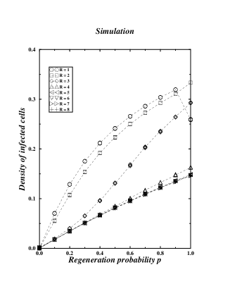
FIG. 1.: Mean density of infected cells $D_{i}$ obtained by simulation for a $L=100$ square lattice as function of the regeneration probability $p$. $R=1-8$, $f/p=0.1$, $q=0.6$. Dashed lines are guide for the eyes.

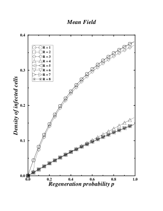
FIG. 2.: Mean density of infected cells $D_{i}$ obtained by mean field approximation, as function of the regeneration probability $p$. Same parameters of figure 1.

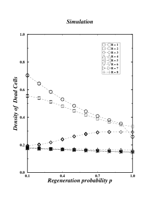
FIG. 3.: Mean density of dead cells $D_{d}$ obtained by simulation on a $L=100$ square lattice as function of the regeneration probability $p$. Same parameters of figure 1.

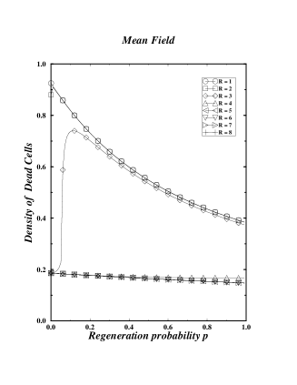
FIG. 4.: Mean density of dead cells obtained by mean field approximation, as function of the regeneration probability. Same parameters of figure 1.

FIG. 5.: Mean density of infected cells $D_{i}$ obtained by the mean field approach as function of the regeneration probability $p$ for $R=3$ for several values from the ratio $f/p=0.0001$ to $1.0$, with $q=0.6$.

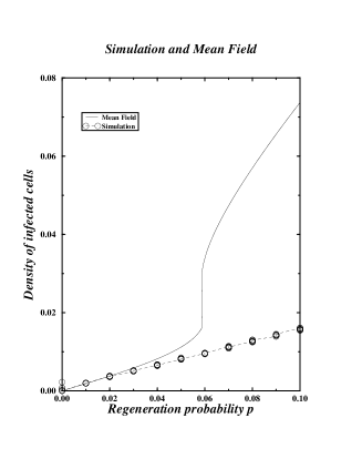
FIG. 6.: Mean density of infected cells $D_{i}$ as function of the regeneration probability $p$ for resistance parameter $R=3$. Full line is obtained from mean field approach and open circles indicates figures from simulations. Same parameters of figure 1.

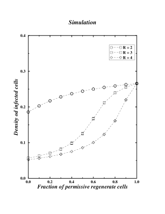
FIG. 7.: Mean density of infected cells $D_{i}$ obtained by simulation on a $L=200$ square lattice as function of the fraction of regeneration of permissive cells $q$ for $f/p=0.1$ and $p=0.6$.

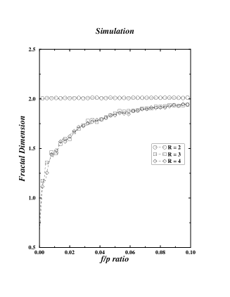
FIG. 8.: Fractal dimension of ulcers contours $D_{F}$ obtained by simulation as function of the $f/p$ ratio for $p=0.01$ and $q=0.6$ on a $L=100$ square lattice, for $R=2,3$ and $4$.

References

References

- [1] G. Landini, G.P. Mission and P.I. Murray, Fractals in the Natural and Applied Sciences, M.M. Novak Ed., Elsevier Science B.V., North Holland (1994);
- [2] A. Hill, P. Jugovic, I. York, G. Russ, J. Bennink, J. Yewdell, H. Ploegh and D. Johnson, Nature, 375, 411, (1995);
- [3] B. Drossel and F. Schwabl, Phys. Rev. Lett. 69, 1629, (1992);
- [4] B. Drossel, S. Clar and F. Schwabl, Phys. Rev. E 50, 1009, (1994).