Analytic Investigations of Random Search Strategies for Parameter Optimization

Abstract

Several standard processes for searching minima of potential functions, such as thermodynamical strategies (simulated annealing) and biologically motivated selfreproduction strategies, are reduced to Schrödinger problems. The properties of the landscape are encoded in the spectrum of the Hamiltonian. We investigate this relation between landscape and spectrum by means of topological methods which lead to a possible classification of landscapes in the framework of the operator theory. The influence of the dimension $d$ of the search space is discussed.

The connection between thermodynamical strategies and biologically motivated selfreproduction strategies is analyzed and interpreted in the above context. Mixing of both strategies is introduced as a new powerful tool of optimization.

I Introduction

The optimization problem appears in several fields of physics and mathematics. It is known from mathematics that every local minimum of a convex function defined over a convex set is also the global minimum of the function. But the main problem is to find this optimum. From the physical point of view every dynamical process can be considered in terms of finding the optimum of the action functional. The best example is the trajectory of the free point mass in mechanics which follows the shortest way between two points.

Let us assume one has successfully set up a mathematical model for the optimization problem under consideration in the form

$$U(x_{1},x_{2},\ldots,x_{d})\longrightarrow\mbox{Min}$$ (1)

where $U$ is a scalar potential function (fitness function) defined over a d-dimensional vector space $X={\cal L}\{x_{1},\ldots,x_{d}\}$. Let $x^{(0)}$ be the absolute Minimum of $U$ which is the search target. Problems of this type are called parameter optimization. Typically the search space is high-dimensional ($d\gg 1$).

The idea of evolution is the consideration of an ensemble of searchers which move through the search space. As a illustrative example we consider the relation between the equation of motion in mechanics, obtained by variation of the action functional $S$ to get a trajectory of minimal action, and the introduction of the probability distribution for all possible trajectories by a functional integral. Because of the weight factor $\exp(-S/\hbar)$ for every trajectory, the trajectory of minimal action has the highest probability. The equation of the probability distribution deduced from the functional integral is the diffusion equation for a free classical particle. The same idea is behind the attempt to describe optimization processes with the help of dynamical processes.

We will be concerned with the time evolution of an ensemble of searchers defined by a density $P(\vec{x},t)$. The search process defines a dynamics

$$P(\vec{x},t+\triangle t)=\mbox{\bf T}[P(\vec{x},t);\triangle t]$$ (2)

with continuous or discrete time steps. An optimization dynamics T is considered as successful, if any (or nearly any) initial density $P(\vec{x},0)$ converges to a target density $\lim\limits_{\tau\rightarrow\infty}P(\vec{x},\tau)$ which is concentrated around the minimum $x^{(0)}$ of $U(\vec{x})$. We restrict ourselves here to the case where T is given as a second order partial differential equation. Among the most successful strategies are the class of thermodynamic oriented [1, 2, 3] and the class of biological oriented strategies [4, 5, 6]). Our aim is to compare on the basis of PDE-models thermodynamical and biologically motivated strategies by reducing both to equivalent eigenvalue problems. Further we introduce a model for mixed strategies and investigate their prospective power [7, 8, 9].

II Thermodynamical Strategies

At first we want to investigate the simplest case of an evolutionary dynamics known in the literature as “simulated annealing”. The analogy between equilibrium statistical mechanics and the Metropolis algorithm [10] was first discussed by Kirkpatrick et al. in [11]. There, an ensemble of searchers determined by the distribution $P(\vec{x},t)$ move through the search space. In the following we consider only the case of a fixed temperature. Then the dynamics is given by the Fokker-Planck equation

$$\frac{\partial}{\partial t}P(\vec{x},t)=\nabla D\cdot[\nabla P+\beta\nabla UP]=D\triangle P+D\nabla(\beta P\nabla U)$$ (3)

with the “diffusion” constant $D$, the reciprocal temperature $\beta$ and the state vector $\vec{x}$. The stationary distribution $P_{0}\sim\exp(-\beta U(\vec{x}))$ is equal to the extremum of functional (12)[12].

For the case $\beta=0$ the complete analytical solution is known and may be expressed by the well-known heat kernel or Green’s function, respectively. The corresponding dynamics is a simulated annealing at an infinite temperature which describes the diffusion process. In this case the optimum of the potential will be found by a random walk, because the diffusion is not sensitive to the potential. The average time which the process requires to move from the initial state $\vec{x}(0)$ to the optimum $\vec{x}^{(0)}$ is given by

$$t_{0}=\frac{1}{D}<(\vec{x}(0)-\vec{x}^{(0)})^{2}>$$ (4)

We note that in several cases a generalization from the number $D=const.$ to the case where $D$ is a symmetrical matrix is possible [12]. Further solvable cases can be extracted from the ansatz

$$P(\vec{x},t)=\exp\left[-\frac{\beta U(x)}{2}\right]y(\vec{x},t)$$ (5)

which after separation of the time and space variables leads to the eigenvalue equation

$$(\epsilon-H)\psi(\vec{x}) = D\triangle\psi(\vec{x})+(\epsilon-V(\vec{x}))\psi(\vec{x})=0$$ (6)

$$y(\vec{x},t) = \exp(-\epsilon t)\psi(\vec{x})$$ (7)

with eigenvalue $\epsilon$ and potential

$$V(\vec{x})=\frac{\beta^{2}}{4}D\nabla U\cdot\nabla U-\frac{\beta}{2}D\triangle U\qquad.$$ (8)

This equation is the well-known stationary Schrödinger equation from quantum mechanics. Under the consideration of a discrete spectrum this leads to the general solution

$$P(\vec{x},t)=\exp\left[-\frac{\beta}{2}U(\vec{x})\right]\sum\limits_{i=0}^{\infty}c_{i}\psi_{i}(\vec{x})\exp(-\epsilon_{i}t)\qquad.$$ (9)

To discuss more properties of equation (6), one has to introduce the concept of the Liapunov functional [13] defined by the formula:

$$\frac{d}{dt}y(\vec{x},t)=-\frac{\delta}{\delta y}{\cal L}(y,\nabla y)\qquad.$$ (10)

In the case of equation

$$\frac{d}{dt}y(\vec{x},t)=D\triangle y(\vec{x},t)-V(\vec{x}))y(\vec{x},t)\qquad,$$ (11)

we obtain

$${\cal L}(y,\nabla y) = \int\limits_{X}L(y,\nabla y)\,dvol(X)$$ (12)

$$L(y,\nabla y) = \frac{D}{2}(\nabla y)^{2}+\frac{1}{2}Vy^{2}\quad.$$ (13)

For the original equation (3), the construction of such functional is impossible.

We remark that the main difference between Schrödinger equation and thermodynamical strategies is given by the time-dependent factor in the solution. In quantum mechanics this set of factors $\exp(i\epsilon t)$ forms a complete basis in the Hilbert space of functions over $t$ but in the solution of (3) this is not the case.

Because of the existence of an equilibrium distribution the first eigenvalue $\epsilon_{0}$ vanishes and the solution is given by

$$P(\vec{x},t)=\mbox{const.}\exp[-\beta U(\vec{x})]\qquad.$$ (14)

That means that the equilibrium distribution is located around the optimum since the exponential $\exp(-U(x))$ is a monotonous function and the optimum is unchanged. In the limit $t\rightarrow\infty$ the distribution $P(\vec{x},t)$ converges to the equilibrium distribution and the strategy successfully terminates at the optimum. But this convergence is dependent on the positiveness of the operator $H$ defined in (6). Usually the Laplace operator is strictly negative definite with respect to a scalar product in the Hilbert space of the square integrable functions ($L^{2}$-space). Therefore the potential alone determines the definiteness of the operator. We thus obtain

$\displaystyle 0<\int\limits_{X}y(x)V(x)y(x)dvol(X)\qquad.$

A sufficient condition for that is

$$\frac{\beta}{2}(\nabla U)^{2}>\triangle U$$ (15)

which means, that the curvature of the landscape represented by $\triangle U$ must be smaller than the square of the gradient. Depending on the potential it thus is possible to fix a subset of $X$ on which the operator $H$ is positive definite.

Now we approximate the fitness function $U(\vec{x})$ by a Taylor expansion around the optimum including the second order. Because the first derivative vanishes one obtains the expression

$$U(x)=U_{min}+\frac{1}{2}\sum\limits_{i=1}^{d}a_{i}(\vec{x}_{i}-\vec{x}_{i}^{(0)})^{2}\qquad.$$ (16)

For $a_{i}>0$ we get the simple harmonic oscillator which is solved by separation of variables. The eigenfunctions are products of Hermitian polynomials with respect to the dimension of the search space. Apart from a constant the same result is obtained in the case $a_{i}<0$. A collection of formulas can be found in appendix A.

The approximation of the general solution (9) for large times leads to

$$P(\vec{x},t)=c_{0}\exp(-\beta U(\vec{x}))+c_{1}e^{-\epsilon_{1}t}\exp\left[-\frac{\beta}{2}U(\vec{x})\right]\psi_{1}(\vec{x})+\ldots$$ (17)

Because of the condition $\epsilon_{2}>\epsilon_{1}$, the time $\tau=1/\epsilon_{1}$ can be interpreted as relaxation time, i.e. the time for the last jump to the optimum. Even more interesting than the consideration of the time is the calculation of velocities. One can define two possible velocities. A first velocity $v^{(1)}$ on the fitness landscape and a second one $v_{k}^{(2)}$ in the $k$-th direction of the search space. The measure of the velocities is given by the time-like change of the expectation values of the vector $x_{k}$ or the potential $U(\vec{x})$, respectively. With respect to equation (3) we obtain

$$v^{(1)}=-\frac{d}{dt}<U>=D\beta<\nabla U\cdot\nabla U>-D<\triangle U>$$ (18)

and

$$v_{k}^{(2)}=-\frac{d}{dt}<x_{k}>=D\beta<\nabla x_{k}\cdot\nabla U>\qquad.$$ (19)

The velocity $v^{(1)}$ depends on the curvature and the gradient. So we can deduce a sufficient condition for a positive velocity

$$\beta(\nabla U)^{2}>\triangle U$$ (20)

which is up to a factor the same as condition (15). For the quadratic potential (16) one obtains

$$|x_{i}-x_{i}^{(0)}|>\frac{1}{\sqrt{a_{i}\beta}}\qquad\forall i\qquad.$$ (21)

This is a restriction to a subset of $X$.

In this case it is also possible to explicitly calculate the velocities for $a_{i}>0$

$$v^{(1)} = \frac{2\,c_{2}}{\beta\,c_{1}}\epsilon_{2}\exp(-\epsilon_{2}t)$$ (22)

$$v_{k}^{(2)} = \sqrt{\frac{2}{\beta a_{k}}}\;\frac{c_{1}}{c_{0}}\,\epsilon_{1}\exp(-\epsilon_{1}t)\qquad.$$ (23)

It is interesting to note that only the first two eigenvalues are important for the velocities and that both velocities vanish in the limit $t\rightarrow\infty$. Besides, the first velocity $v^{(1)}$ is independent of the parameter $a_{i}$ except for special initial conditions where the factor $c_{k}$ depends on the parameter $a_{i}$. The other case $a_{i}<0$ is similar and can be found in appendix A.

III Fisher-Eigen Strategies

In principle, the biologically motivated strategy is different from the thermodynamical strategy. Whereas in the thermodynamical strategy the population size remains constant, it is changed with respect to the fundamental processes reproduction and selection in the case of biologically motivated strategies, but is kept unchanged on average. The simplest model with a similar behaviour is the Fisher-Eigen equation given by

$$\frac{\partial}{\partial t}P(\vec{x},t) = [<U>-U(\vec{x})]P(\vec{x},t)+D\triangle P(\vec{x},t)$$ (24)

$$<U>(t) = \frac{\int U(x)P(\vec{x},t)dx}{\int P(\vec{x},t)dx}$$ (25)

In this case one can also form a Liapunov functional which satisfies the equation (10) similar to the thermodynamical strategy. One obtains the positive functional

$${\cal L}=\int\limits_{X}\left(\frac{D}{2}(\nabla P)^{2}-\frac{1}{2}(<U>-U)P^{2}\right)\,dvol(X)$$ (26)

which also has the stationary distribution as an extremum.

By using the ansatz

$$P(\vec{x},t)=\exp\left[\int\limits_{0}^{t}<U>(t^{\prime})dt^{\prime}\right]y(\vec{x},t)$$ (27)

and the separating time and space variables, the dynamics reduces to the stationary Schrödinger equation

$$(\epsilon_{i}-H)\psi_{i}(\vec{x})=D\triangle\psi_{i}(\vec{x})+[\epsilon_{i}-U(\vec{x})]\psi_{i}(\vec{x})=0$$ (28)

where $\epsilon_{i}$ are the eigenvalues and $\psi_{i}(\vec{x})$ are the eigenfunctions. This leads to the complete solution

$$y(\vec{x},t)=\sum\limits_{i}a_{i}e^{-\epsilon_{i}t}\psi_{i}(\vec{x})\qquad.$$ (29)

The difference to the thermodynamical strategy is given by the fact that the eigenvalue $\epsilon_{0}$ in the case of the Fisher-Eigen strategy is a non zero value, i.e. the relaxation time is modified and one obtains

$$t_{0}=\frac{1}{\epsilon_{1}-\epsilon_{0}}\qquad.$$ (30)

For the harmonic potential (16) the problem is exactly solvable for any dimension $d$ and the solution is very similar to the thermodynamical strategy for $a_{i}>0$. In the other case $a_{i}<0$ we obtain a different problem known from scattering theory. If the search space is unbound the spectrum of the operator $H$ is continuous. From the physical point of view we are interested in positive values of the potential or fitness function (16), respectively. This leads to a compact search space given by the interval $[-b,b]$ in each direction with $b=\sqrt{2U_{min}/|a_{i}|}$. We now have to introduce boundary conditions. The most natural choice is to let the solution vanish on the boundary. As a result an additional restriction appears and the spectrum of the operator $H$ is now discrete. A collection of formulas connected to both eigenvalue problems can be found in appendix B.

The next step is the calculation of the velocities defined in the previous section. With respect to the Fisher-Eigen equation (24) one obtains

$$v^{(1)} = <U^{2}>-<U>^{2}-D<\triangle U>$$ (31)

$$v_{k}^{(2)} = <x_{k}U>-<x_{k}><U>\qquad.$$ (32)

For the case of a quadratic potential all velocities can be calculated from the solution and with $a_{i}>0$ the following expansion is possible:

$$v^{(1)} = 4D\epsilon_{0}+O(e^{(-(\epsilon_{2}-\epsilon_{0})t)})$$ (33)

$$v_{i}^{(2)} = \sqrt{\frac{18D}{a_{i}}}\frac{c_{1}}{c_{0}}\epsilon_{1}e^{(-(\epsilon_{1}-\epsilon_{0})t))}+O(e^{(-(\epsilon_{3}-\epsilon_{0})t)})\qquad.$$ (34)

These velocities are very similar to the velocities of the thermodynamical strategy. So it is very difficult to decide whether or not the thermodynamical strategy is faster than the biologically motivated one or vice versa. This decision depends on the particular circumstances. The thermodynamical strategy is faster than the biologically motivated one in a landscape with a slight curvature and widely extended hills whereas the biological strategy needs a landscape with a high curvature and more localized hills to be faster than the thermodynamical strategy.

We note the interesting fact, that there exist special tunnel effects connected with minima of equal depth and shape. The corresponding spectrum of the Hamiltonian shows degenerated eigenvalues. Then under the condition of overlapping distributions located in different minima an tunnelling with high probability between these minima is possible (see Fig. 1, dotted line). For the corresponding Boltzmann strategy the transformed potential does not admit this tunnelling effect (Fig. 1, solid line).
FIG. 1.: The double well problem for Fisher-Eigen and Boltzmann

IV Mixed Boltzmann–Darwin Strategies

The dynamic equations defining Boltzmann–type search and Fisher–Eigen type search contain a common term $D\triangle P$. Since both types of strategies have definite advantages and disadvantages it seems desirable to mix them. We defined the dynamics of a mixed strategy by

$$\frac{\partial}{\partial t}P(\vec{x},t) = D\triangle P(\vec{x},t)+\beta D\nabla(P\nabla U)$$ (35)

$$+ \gamma[<U>-U(\vec{x})]P(\vec{x},t)$$ (36)

For $\gamma=0$ this dynamics reduces to a pure Boltzmann strategy and for $\beta=0$ we obtain a Fisher–Eigen strategy. The mixed case may be treated by means of the ansatz

$$P(\vec{x},t)=\exp\left[\gamma\int\limits_{0}^{t}<U>dt^{\prime}-\frac{1}{2}\beta U(\vec{x}\right]y(\vec{x},t)$$ (37)

which leads to the explicit solution in the eigenfunctions of the problem

$$0 = D\triangle\psi_{i}(\vec{x})+[\epsilon_{i}-E(\vec{x})]\psi_{i}(\vec{x})$$ (38)

$$E(\vec{x}) = \gamma U-\frac{D\beta}{2}\triangle U+\frac{D\beta^{2}}{4}(\nabla U)\cdot(\nabla U)\qquad.$$ (39)

For $\beta=0$ and $\gamma=1$ we end up with the case of Fisher-Eigen strategies and for $\gamma=0$ , $\beta>0$ the Boltzmann dynamics is obtained. In this respect the mixed strategy is indeed a generalization of both cases (see Fig. 2).
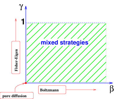
FIG. 2.: The parameter dependence of the mixed strategy
The linearity of the differential equation leads to simple relations between the solutions and velocities. For instance the velocities for the thermodynamical and the biological strategy can be added with respect to the constant $\gamma$ to get the velocities of the mixed strategy. For the solution of the problem one simply takes the solution of the thermodynamical strategy (51) and redefines the coordinate $\xi_{k}$ by

$\displaystyle\xi_{k}=x_{k}\sqrt[4]{\frac{\beta^{2}\,a_{k}^{2}}{4}+\frac{\gamma\,a_{k}}{2D}}\qquad.$

So the mixed strategy combines the advantages of both strategies if one uses a criterion to choose the coefficients $\gamma$ and $\beta$. The dependence on the 3 optimization parameters $D$, $\beta$ and $\gamma$ is a rather simple one. For a given $D$, the best strategy is evidently an increase of the $\beta$-value, since the $\gamma$-dependence is weak. However, if the “friction” $\beta D$ is fixed by the conditions, the maximization of $\gamma/\beta$ leads to the smallest relaxation time. In other words, if the loss $\beta D$ is fixed, maximal $\gamma$ (i.e. most competition) and minimal $\beta$ (i.e. large temperature) is the best choice for a fast search of the minimum. In general the optimal search requires $\beta>0$ and $\gamma>0$. With other words, adding some amount of the “complementary” strategy is in most cases to be recommended. This was already found empirically in a earlier work [7, 8].

V Global properties of Strategies

The study of the problem given by the potential (16) is the same as the study of the local properties of the landscape. It is known from the Lemma of Morse, that there is a coordinate system so that every function with non-degenerate critical points in the neighborhood $U_{p}$ of one critical point $p$ can be expressed as

$\displaystyle f=f(p)-(y_{1})^{2}-\ldots-(y_{\lambda})^{2}+(y_{\lambda+1})^{2}+\ldots+(y_{d})^{2}$

with $(y_{1},\ldots,y_{d})$ as coordinate system. The number $\lambda$ is the index of the critical point. Now we use the compact space $X\cup\{\infty\}$ rather than $X={\mbox{\rm I\kern-1.99997ptR}}^{d}$ which in contrast to ${\mbox{\rm I\kern-1.99997ptR}}^{d}$ is homeomorphic to $S^{d}$, the $d$-dimensional sphere. Now every function over $S^{d}$ is non-degenerate and we obtain for the number $C_{\lambda}$ of critical points with index $\lambda$ the Morse inequalities [14]

$$1\leq C_{0}\qquad 1 \leq C_{d}\qquad 0\leq C_{\iota}$$ (40)

$$1+(-1)^{d} = \sum\limits_{\lambda}(-1)^{\lambda}C_{\lambda}$$ (41)

with $\iota=1,\ldots d-1$. So we find that in the case of many maxima and minima the number of saddle points increases [15]. This is a global statement which only depends on the topology of the sphere $S^{d}$.

In the case of a compact, simple-connected subset of ${\mbox{\rm I\kern-1.99997ptR}}^{d}$ one obtains a similar result because the boundary of this subset is homeomorphic to a $d-1$ dimensional sphere and the Morse inequalities can be used again. If this subset has no boundary then we obtain

$$1=\sum\limits_{\lambda}(-1)^{\lambda}C_{\lambda}$$ (42)

and the result of [15] can be deduced again. The treatment of constraints in the optimization problem is connected with the occurrence of holes in the space. This leads to a correction of the formulas (41) or (42), respectively. The number of saddle points increases with respect to the number of holes.

Next we want to study the influence of the landscape on the solutions in terms of the dynamics, which in our case is restricted to the influence of the potential or fitness function, respectively. The general form of this dynamics is given by

$$\frac{\partial}{\partial t}P(x,t)=-HP(x,t)$$ (43)

with the selfadjoint Operator

$$H_{B} = -D\nabla\cdot(\nabla+\beta\nabla U)\qquad\mbox{Boltzmann}$$ (44)

$$H_{FE} = -<U>+U-D\triangle\qquad\mbox{Fisher-Eigen}\qquad.$$ (45)

This operator equation has the formal solution

$$P(x,t)=\exp(-tH)P(x,0)$$ (46)

acting on the initial condition. With the help of (27), the operator for the Fisher-Eigen strategy can be reduced to $H=U-D\triangle$. Then both operators are in the same class known as generalized Laplacian. The representation of this class from a unified point of view is possible. To this end we introduce the Dirac operator as a first order differential operator and regard the generalized Laplacian $H$ as the square of the Dirac operator. It was shown in [16] that every generalized Laplacian can be represented by the square of a Dirac operator with respect to a suitable Clifford multiplication. For the two cases one obtains

$$D_{B} = i\gamma^{\mu}(\partial_{\mu}+\partial_{\mu}U)\qquad\mbox{Boltzmann}$$ (47)

$$D_{FE} = \gamma^{\mu}(\partial_{\mu}+iA_{\mu}(x))\qquad\mbox{Fisher-Eigen}$$ (48)

where $\gamma^{\mu}$ are the Dirac matrices ($\mu=1,\ldots d$) and $A_{\mu}(x)$ is a locally defined vector field with $[\gamma^{\mu},\gamma^{\nu}]\partial_{\mu}A_{\nu}(x)=-iU(x)$. Together with the expression

$$D=\left(\begin{array}[]{cc}0&{/\mkern-10.0mu\partial}\\ {/\mkern-10.0mu\partial}^{*}&0\end{array}\right)$$ (49)

for every Dirac operator $D$, one can simple calculate the squares of the Dirac operators to establish

$$H_{B}=D_{B}^{2}=\left(\begin{array}[]{cc}{/\mkern-10.0mu\partial}_{B}{/\mkern-10.0mu\partial}_{B}^{*}&0\\ 0&{/\mkern-10.0mu\partial}_{B}^{*}{/\mkern-10.0mu\partial}_{B}\end{array}\right)\qquad H_{FE}=D_{FE}^{2}$$ (50)

with the adjoint operator ${/\mkern-10.0mu\partial}^{*}$. This means that both problems can be described by the motion of a fermion in a field $\nabla U$ or $iA(x)$, respectively. The equilibrium state (or stationary state) is given by the kernel of the operator $H$ which is the direct sum $\ker H=\ker{/\mkern-10.0mu\partial}\oplus\ker{/\mkern-10.0mu\partial}^{*}$. If the dimension $d$ is even, which is always true for the high-dimensional case, this splitting can be introduced by the product of all $\gamma$-matrices usually denoted by $\gamma^{5}$. Because of the compactness of the underlying space $S^{d}$, the kernel of $H$ is finite-dimensional and the spectrum is discrete. We note, that the spectrum of both, ${/\mkern-10.0mu\partial}{/\mkern-10.0mu\partial}^{*}$ and ${/\mkern-10.0mu\partial}^{*}{/\mkern-10.0mu\partial}$, is equal up to the kernel. So the interesting information about the problem is located in the asymmetric splitting of the kernel $\ker H$. The physical interpretation is given by an asymmetric ground state of the problem which is only connected to the geometry of the landscape. In more mathematical terms both Dirac operators are described as covariant derivatives with a suitable connection. Together with the fiber bundle theory [17] and the classification given by the K-theory [18] one obtains a possible classification of the fitness landscapes in dependence of convergence velocities given by the periodicity of the real K-theory with period 8. Each of these 8 classes describes a splitting of the kernel $\ker H$ and leads to a different velocity. A complete description of this problem will be published later on.

VI Conclusions

In physics the most classical dynamical processes follow the principle of minimization of a physical quantity which often leads to an extremum of the action functional. This problem frequently has a finite number of solutions given by the solutions of a differential equation also known as the equation of motion. Investigating this fact in relation to optimization processes, one obtains in the simplest case the thermodynamical and the biological strategy. The description is given by the distribution of the searcher and a dynamics of the distribution converging to an equilibrium distribution located around the optimum of the optimization problem. With the help of the kinetics and the eigenfunction expansion, we investigated both strategies in view of the convergence velocity. In principle both strategies are equal because one obtains a stationary Schrödinger equation. But, the main difference is the transformation of the fitness function (or potential) from $U(x)$ to $V(x)$ (see (8)) in the case of the thermodynamical strategy. The difference of both strategies leads to the idea of adding a small amount of the “complementary” strategy in order to hope for an improvement. The difference in the velocity on the one hand and the similarity in the equation on the other look like a unified treatment of both strategies under consideration. This is represented in the last section in the formalism of fiber bundles and heat kernels to get the interesting result, that up to local coordinate transformations the strategies are split into 8 different classes.

A - Thermodynamical strategy

For the case of quadratic potentials (16) the problem (3) may be solved explicitly. We get the eigenvalues

$\displaystyle\epsilon_{n_{1}\ldots n_{d}}=U_{min}+\sum\limits_{i=1}^{d}a_{i}\beta D\left(n_{i}+\frac{1}{2}\right)\qquad n_{i}=0,1,2,\ldots$

and the eigenfunctions

$$\psi_{n_{1}\ldots n_{d}}(x_{1},\ldots,x_{d})=\prod\limits_{i=1}^{d}\psi_{n_{i}}(x_{i})$$

$$\psi_{n_{i}}(x_{i})=\exp\left(-\frac{\beta a_{i}}{4}x_{i}^{2}\right)H_{n_{i}}\left(\sqrt{\frac{\beta a_{i}}{2}}x_{i}\right)$$

which lead to the solution

$$P(\vec{x},t)=\sum\limits_{i=n_{1}+\ldots+n_{d}}c_{i}\prod\limits_{k=1}^{d}\left[\exp(-\xi_{k}^{2})H_{n_{k}}(\xi_{k})\right]\exp(-\epsilon_{i}t)$$ (51)

with $\xi_{k}=x_{k}\,\sqrt{\beta a_{k}/2}$. Next we have to fix initial conditions for this problem. At first one starts with a strong localized function, i.e. with a delta distribution.

$\displaystyle P(\vec{x},0)=\prod\limits_{i=1}^{d}\delta(x_{i}-x^{(0)}_{i})$

Because of the relation:

$$\int\exp(-\xi^{2})H_{n}(\xi)H_{m}(\xi)d\xi=\delta_{mn}\int\exp(-\xi^{2})H^{2}_{n}(\xi)d\xi=\delta_{mn}N_{n}=\delta_{mn}2^{n}(n!)\sqrt{\pi}$$ (52)

we obtain for the coefficients

$$c_{k}=\prod\limits_{i=1}^{d}\frac{2}{N_{n_{i}}\beta a_{i}}H_{n_{i}}\left(\sqrt{\beta a_{i}}{2}x^{(0)}_{i}\right)\qquad.$$ (53)

with $k=n_{1}+n_{2}+\ldots+n_{d}$. In the case of the full symmetry $a=a_{1}=a_{2}=\ldots=a_{d}$ we can calculate the radial problem to obtain the eigenvalues

$\displaystyle\epsilon=a\beta Dd\left(k+\frac{1}{2}\right)$

with $d$ as the dimension of the landscape. The calculation of the velocities leads to two cases for the potential (16):

1. $a_{i}>0$

   $$v^{(1)} = \frac{2\,c_{2}}{\beta\,c_{1}}\epsilon_{2}\exp(-\epsilon_{2}t)$$ (54)

   $$v_{k}^{(2)} = \sqrt{\frac{2}{\beta a_{k}}}\;\frac{c_{1}}{c_{0}}\,\epsilon_{1}\exp(-\epsilon_{1}t)$$ (55)

2. $a_{i}<0$

   $$v^{(1)} = \frac{2}{\beta N_{1}}\sum\limits_{k=0}^{\infty}c_{2k}\exp(-\epsilon_{2k}t)\epsilon_{2k}\sum\limits_{i=1}^{d}\frac{H_{2k+3}(b_{i})}{(2k+1)(2k+2)(2k+3)}\prod\limits_{j=1\,i\not=j\atop k_{1}+\ldots k_{d}=k}^{d}\frac{H_{2k_{i}+1}(b_{j})}{(2k+1)}$$ (56)

   $$v_{i}^{(2)} = \sqrt{\frac{2}{\beta a_{k}}}\;\frac{1}{N_{1}}\sum\limits_{k=0}^{\infty}c_{2k+1}\exp(-\epsilon_{2k+1}t)\epsilon_{2k+1}\frac{H_{2k+3}(b_{i})}{(2k+2)(2k+3)}\prod\limits_{j=1\,i\not=j\atop k_{1}+\ldots k_{d}=k}^{d}\frac{H_{2k_{i}+1}(b_{j})}{(2k+1)}$$ (57)

where

$\displaystyle N_{1}=\sum\limits_{k=0}^{\infty}c_{2k}\exp(-\epsilon_{2k}t)\prod\limits_{i=1\atop k_{1}+\ldots k_{d}=k}^{d}\frac{H_{2k_{i}+1}(b_{i})}{(2k+1)}$

is the normalization factor and $b_{i}=\sqrt{2U_{m}/a_{i}}$ is the interval length.

B - Biological strategy

For a harmonic potential (16) the problem (24) is exactly solvable for any dimension $d$. We get the eigenvalues

$\displaystyle\epsilon_{n_{1}\ldots n_{d}}=U_{min}+\sum\limits_{i=1}^{d}\sqrt{2a_{i}\,D}\left(n_{i}+\frac{1}{2}\right)\qquad n_{i}=0,1,2,\ldots$

and the eigenfunctions

$$\psi_{n_{1}\ldots n_{d}}(x_{1},\ldots,x_{d})=\prod\limits_{i=1}^{d}\psi_{n_{i}}(x_{i})$$

$$\psi_{n_{i}}(x_{i})=\exp\left(-\sqrt{\frac{a_{i}}{4D}}x_{i}^{2}\right)H_{n_{i}}\left(\sqrt[4]{\frac{a_{i}}{2D}}x_{i}\right)$$

which lead to the solution

$$P(\vec{x},t)=\sum\limits_{i=n_{1}+\ldots+n_{d}}c_{i}\prod\limits_{k=1}^{d}\left[\exp\left(-\frac{\xi_{k}^{2}}{2}\right)H_{n_{k}}(\xi_{k})\right]\exp(-\epsilon_{i}t)$$ (58)

with $\xi_{k}=x_{k}\,\sqrt[4]{a_{k}/(2D)}$.

We now come to the problem of the maximum, i.e. the potential (16) with $a_{i}<0$. The solution for one dimension (direction $i$) is simply obtained as

$$\psi_{\lambda_{i}}(x_{i})=D_{-iB_{i}-\frac{1}{2}}\left(\sqrt[4]{\frac{a_{i}}{2D}}\;e^{-i\pi/4}x_{i}\right)$$ (59)

with $B_{i}=\lambda_{i}/(2\sqrt{Da_{i}})$ and $D_{k}(x)$ as parabolic Bessel functions depending on the parameter $B_{i}$. In practice one is interested in positive values of the fitness function or potential which leads to a restriction of the search space $X$ to the a hypercube with length $b_{i}=\sqrt{2U_{m}/a_{i}}$ in every dimension. We claim that the solution vanishes at the boundary of the hypercube. This restriction leads to a discrete spectrum. The zeros of the parabolic Bessel function are given by the solution of the equation

$$\frac{1}{4}\left(\rho_{ki}\sqrt{\rho_{ki}^{2}-1}-\mbox{arccosh}\,\rho_{ki}\right)=\frac{(-A_{n})^{3/2}}{6\sqrt{\frac{U_{m}+n_{i}}{2\sqrt{a_{i}D}}}}$$ (60)

where the coefficients $A_{i}$ can be found in the book [19] and the zeros are defined by $c=2\sqrt{a_{i}}\rho$. For the eigenvalues $\epsilon_{k}$ in (28) one obtains

$$\epsilon_{n}=\sum\limits_{i=1\atop n_{1}+\ldots n_{d}=n}^{d}n_{i}\qquad\qquad n_{i}=\frac{U_{m}}{\rho_{ki}^{2}}\sqrt{\frac{D}{a_{i}}}-U_{m}\qquad.$$ (61)

The calculation of the velocities is very lengthy and one obtains

1. $a_{i}>0$ (minimum):

   $$v^{(1)} = \frac{1}{N_{1}}\sum\limits_{i=1}^{d}\sqrt{\frac{Da_{i}}{2}}\left(c_{0}\epsilon_{0}e^{-\epsilon_{0}t}+\sum\limits_{k=1}^{\infty}(-1)^{k+1}\frac{(2k)!}{k!}(2k^{2}+k+\frac{3}{2})c_{2k}\epsilon_{2k}e^{-\epsilon_{2k}t}\right)$$ (62)

   $$v_{i}^{(2)} = \sqrt{\frac{2D}{a_{i}}}\frac{3}{N_{1}}\left(\sum\limits_{k=0}^{\infty}(-1)^{k}\frac{(2k+1)!}{k!}c_{2k+1}\epsilon_{2k+1}\exp(-\epsilon_{2k+1}t)\right)$$ (63)

   with

   $$N_{1}=\sum\limits_{k=0}^{\infty}(-1)^{k}\frac{(2k)!}{k!}c_{2k}\exp(-\epsilon_{2k}t)$$ (64)

   as normalization.

2. case $a_{i}<0$ (maximum):

   $$v^{(1)} = \frac{1}{N_{2}}\sum\limits_{n=1\atop n_{1}+\ldots n_{d}=n}^{\infty}\epsilon_{n}e^{\epsilon_{n}t}\prod\limits_{i=1}^{d}\left(\sqrt{\left|\frac{\Gamma(\frac{1}{4}+ib_{i}/2)}{\Gamma(\frac{3}{4}+ib_{i}/2)}\right|}\right)\sum\limits_{k=1}^{d}I_{k}(\xi_{k}^{2})\sqrt{\frac{D\,|a_{k}|}{2}}$$ (65)

   $$v_{k}^{(2)} = \frac{1}{N_{2}}\sum\limits_{n=1\atop n_{1}+\ldots n_{d}=n}^{\infty}\epsilon_{n}e^{\epsilon_{n}t}\prod\limits_{i=1}^{d}\left(\sqrt{\left|\frac{2\Gamma(\frac{3}{4}+ib_{i}/2)}{\Gamma(\frac{1}{4}+ib_{i}/2)}\right|}I_{i}()\right)I_{k}(\xi_{k})\sqrt[4]{\frac{|a_{k}|}{2D}}$$ (66)

   with

   $$I_{k}(\xi_{k}) = \int\limits_{-u_{k}}^{u_{k}}\xi_{k}y_{1}(\xi_{k})d\xi_{k}\qquad I_{k}(\xi_{k}^{2})=\int\limits_{-u_{k}}^{u_{k}}\xi_{k}^{2}y_{2}(\xi_{k})d\xi_{k}\qquad I_{k}()=\int\limits_{-u_{k}}^{u_{k}}y_{1}(\xi_{k})d\xi_{k}$$ (67)

   $$u_{k} = \frac{2U_{m}}{|a_{k}|}\sqrt[4]{\frac{|a_{k}|}{2D}}\qquad\qquad b_{k}=\frac{n_{k}}{2\sqrt{D|a_{k}|}}$$ (68)

   $$N = \sum\limits_{n=1\atop n_{1}+\ldots n_{d}=n}^{\infty}e^{\epsilon_{n}t}\prod\limits_{i=1}^{d}\left(\sqrt{\left|\frac{\Gamma(\frac{1}{4}+ib_{k}/2)}{\Gamma(\frac{3}{4}+ib_{k}/2)}\right|}\,I_{k}()\,\right)$$ (69)

   and functions $y_{1}(),y_{2}()$ defined in [19] page 692 as series

   $$y_{1}(\xi_{k}) = 1+b_{k}\frac{\xi_{k}^{2}}{2!}+\left(b_{k}^{2}-\frac{1}{2}\right)\frac{\xi_{k}^{4}}{4!}+\ldots$$ (70)

   $$y_{2}(\xi_{k}) = \xi_{k}+b_{k}\frac{\xi_{k}^{3}}{3!}+\left(b_{k}^{2}-\frac{3}{2}\right)\frac{\xi_{k}^{5}}{5!}+\ldots$$ (71)

REFERENCES

- [1] J.D. Nulton and P. Salamon. Statistical mechanics of combinatorical optimization. Phys. Rev., A 37:1351, 1988.
- [2] B. Andresen. Finite-time thermodynamics and simulated annealing. In Proceedings of the Fourth International Conference on Irreversible Processes and Selforganization, Rostock, 1989.
- [3] P. Sibiani, K.M. Pedersen, K.H. Hoffmann, and P. Salamon. Monte Carlo dynamics of optimization: A scaling description. Phys. Rev., A 42:7080, 1990.
- [4] H.P. Schwefel. Evolution and optimum seeking. Wiley, New York, 1995.
- [5] I. Rechenberg. Evolutionsstrategien - Optimierung technischer Systeme nach Prinzipien der biologischen Information. Friedrich Frommann Verlag (Günther Holzboog K.G.), Stuttgart - Bad Cannstatt, 1995.
- [6] R. Feistel and W. Ebeling. Evolution of Complex Systems. Kluwer Academic Publ., Dordrecht, 1989.
- [7] W. Ebeling and A. Engel. Models of Evolutionary systems and their applications to optimization problems. Syst. Anal. Model. Simul., 3:377, 1986.
- [8] T. Boseniuk, W. Ebeling, and A. Engel. Boltzmann and Darwin strategies in complex optimization. Phys. Lett., A 125:307, 1987.
- [9] T. Boseniuk and W. Ebeling. Boltzmann- , Darwin- and Heackel-strategies in optimization problems. In PPSN Dortmund, 1990.
- [10] N. Metropolis, A. Rosenbluth, M. Rosenbluth, A. Teller, and E. Teller. J. Chem. Phys., 21:1087, 1953.
- [11] S. Kirkpatrick, C.D. Gelatt Jr., and M.P. Vecchi. Science, 220:671, 1983.
- [12] H. Risken. The Fokker-Planck Equation. Springer Verlag, 1989.
- [13] G. Jetschke. Mathematik der Selbstorganisation. Deutscher Verlag der Wissenschaften, 1989.
- [14] J. Milnor. Morse theory. Ann. of Mathematical Study 51. Princeton Univ. Press, Princeton, 1963.
- [15] M. Conrad and W Ebeling. M.V. Volkenstein, evolutionary thinking and the structue of fitness landscapes. BioSystems, 27:125, 1992.
- [16] N. Berline, M. Vergne, and E. Getzler. Heat kernels and Dirac Operators. Springer Verlag, New York, 1992.
- [17] D. Husemoller. Fiber Bundles. MacGraw-Hill Book Co., New York-London-Sydney, 1966.
- [18] M. Atiyah. K-Theory. W.A. Benjamin, New York–Amsterdam, 1967.
- [19] Milton Abramowitz and Irene A. Stegun. Handbook of Mathematical Functions with Formulas, Graphs, and Mathematical Tables. Applied Mathematical Series 55. National Bureau of Standards, December 1972.