Cellular Games

Abstract

A cellular game is a dynamical system in which cells, placed in some discrete structure, are regarded as playing a game with their immediate neighbors. Individual strategies may be either deterministic or stochastic. Strategy success is measured according to some universal and unchanging criterion. Successful strategies persist and spread; unsuccessful ones disappear.

In this thesis, two cellular game models are formally defined, and are compared to cellular automata. Computer simulations of these models are presented.

Conditions providing maximal average cell success, on one and two-dimensional lattices, are examined. It is shown that these conditions are not necessarily stable; and an example of such instability is analyzed. It is also shown that Nash equilibrium strategies are not necessarily stable.

Finally, a particular kind of zero-depth, two-strategy cellular game is discussed; such a game is called a simple cellular game. It is shown that if a simple cellular game is left/right symmetric, and if there are initially only finitely many cells using one strategy, the zone in which this strategy occurs has probability $0$ of expanding arbitrarily far in one direction only. With probability $1$, it will either expand in both directions or disappear.

Computer simulations of such games are presented. These experiments suggest the existence of two different kinds of asymptotic behavior.

To My Mother, Dinah Green Levine

Table of Contents

toc

List of Figures

1. D.1 Computer simulation of the Stag Hunt, a modified Arthur-Packard- Rogers cellular game model, with $75$ cells, and $150$ generations per round. Program cg2.pas, random seed $824709136$, generation 1. In this program, all initial strategies are depth $1$, but strategies of depth up to $3$ may be introduced as the system evolves.
2. D.2 The same program, parameters, and seed as above, generation $27$. Notice the rightward-moving waves of cooperative behavior, in the right part of the display. Here some zones exhibit cellular automaton-like triangular patterns.
3. D.3 Generation $139$ of this run. Cellular automaton-like triangles predominate in this figure.
4. D.4 Generation $165$. There are now leftward-moving waves of cooperative behavior, in the middle of the display.
5. D.5 Generation $305.$
6. D.6 Generation $483$. Cellular automaton-like triangles appear again.
7. D.7 Generation $560$. Move behavior does not appear to have changed much in many generations.
8. D.8 Generation $561$. An all-cooperate zone appears. The next three figures show the rapid growth of this zone.
9. D.9 Generation $612$.
10. D.10 Generation $658$.
11. D.11 Generation $662$. The all-cooperate zone has almost completely taken over the ring.
12. D.12 Generation $930$. Large all-cooperate zones have predominated in the past several hundred generations. However, at this point, a perturbation in strategy – that is, an unexpected defect move – can set off many defect moves in other cells.
13. D.13 Generation $982$. Recovery of an all-cooperate zone.
14. D.14 Generation $1262$. At this point, perturbations do not set off much defecting behavior in other cells. That is, strategies are no longer, “Cooperate unless there are defectors in the neighborhood,” but, “Cooperate, whatever happens.”
15. D.15 Computer simulation of a one-round cellular game, the Cloud Process, on a ring of $640$ cells. The table for this game is: $G(BBB)=G(WWW)=0.27$, $G(BBW)=G(BWB)=G(BWW)=G(WBB)=G(WBW)=G(WWB)=0.53$. Program cloud.pas, random seed $118950941$. Initial conditions were chosen with the aid of a pseudorandom number generator.
16. D.16 Computer simulation of a one-round Prisoner’s Dilemma game on a ring of $600$ cells. Initially, two defectors are placed side-by- side; all other cells are cooperators. (Black indicates defecting cells, and white, cooperating.) Program prisoner.pas, random seed $424479774$. Note that the rate of expansion of the black domain appears roughly similar on each side, thus suggesting an informal estimate of the expected rate.
17. D.17 Computer simulation of a zero-depth, one round per generation Stag Hunt game on a ring of $600$ cells. Initially, four cooperators are placed contiguously; all other cells are defectors. Program stag.pas, random seed $941165838$. Note that, in this case, the rate of expansion of the white domain appears to vary considerably.
18. D.18 Computer simulation of a zero-depth, one round per generation Stag Hunt game on a ring of $600$ cells. Initially, four defectors are placed contiguously; all other cells are cooperators. Program stag2.pas, random seed $90049811$.
19. D.19 Join/mix processes with various parameters. Each process is run on a circular lattice of $165$ cells for $125$ generations. Initially, all cells are white except for cells $48$ through $70$, and $95$ through $117$. The numbers at the bottom show the values of $p_{1}$; and those on the left show the values of $p_{2}$. That is, both $p_{1}$ and $p_{2}$ are set at $0.15$, $0.50$, and $0.85$. The program used is square.pas, seed $252644401$.
20. D.20 Computer simulation of the Join or Die Process on a ring of $640$ cells. Initial conditions are black for cells $0$ through $127$, and $512$ through $639$, and white for cells $128$ through $511$. Program jd.pas, random seed $274535429$.
21. D.21 Computer simulation of the Join or Die Process. Initial conditions were chosen with the aid of a pseudorandom number generator, so each cell is equally likely to be black or white. Random seed $705238026$ is used; and the same program, and ring size, as in the preceding figure.
22. D.22 The annihilating particle model, on a ring of $640$ cells, which initially contains $28$ particles. Program apm.pas, seed $269093635$. Each particle executes a symmetric random walk, having a $50\%$ probability of going either left or right in each generation.
23. D.23 Computer simulation of the Mixing Process on a ring of $640$ cells. Initial conditions are black for cells $0$ through $127$, and $512$ through $639$, and white for cells $128$ through $511$. Program mix.pas, random seed $912200719$.

Chapter 1 Introduction

A cellular game is a dynamical system; that is, the variables it is composed of are regarded as changing over time. These variables or cells, arranged in a discrete structure such as a ring, are thought of as repeatedly playing a game with their neighbors. Most of this paper is concerned with one-dimensional cellular games, defined more formally as follows:

Definition 1.1

A one-dimensional cellular game consists of:

1. A one-dimensional discrete structure, uniform from the viewpoint of each site; that is, a ring or doubly infinite path.

2. A variable, or cell, at each site. The components of this variable may change at each discrete unit of time, or round. They consist of, at least:

   1. A move component, which can take on a finite number $k$ of values.

   2. A strategy component, which determines what move a cell makes in a given round. The strategy of a cell is based on past moves of it and its $r$ nearest neighbors on each side. The number of past rounds considered is called the depth $d$ of the strategy. This $r$, as used above, is the radius of the game.

3. A fitness criterion, which does not change and is the same for each cell. This fitness criterion is usually local; that is, the fitness of a cell in each round is based on its move, and those of nearest neighbors within the radius of the game.

4. A mechanism for strategy selection, under which more fit strategies survive and spread. Strategy selection is usually nonlocal; that is, a more fit strategy may spread arbitrarily far in a fixed number of time units. An interval between strategy changes, which may be one or more rounds, is called a generation.

Thus, a cellular game can be considered a process in which cells make moves each round, based on their strategies, and strategies are updated in each generation, based on their fitness in preceding rounds.

Note that cellular game strategies and fitness criteria are usually stored in the form of a table. Also note that $n$-dimensional cellular automata, with one cell for each $n$-tuple of integers or integers mod $k$, can be similarly defined.

One-dimensional cellular games are studied in [20], [3], [4], and [13]. Similar systems are discussed in [10], [11] and [12]; and games on a two-dimensional lattice in [15].

Cellular games satisfy a criterion for “artificial life” as discussed by Christopher Langton [7]. That is, “There are no rules in the system that dictate global behavior. Any behavior at levels higher than the (individual cells) is, therefore, emergent.”

Cellular games are a generalization and extension of another, more well-known, discrete dynamical system; that is, of cellular automata. They were created largely because of questions arising from the observation of cellular automata. One-dimensional cellular automata are defined as follows:

Definition 1.2

A one-dimensional cellular automaton consists of:

• A one-dimensional discrete structure, uniform from the viewpoint of each site; that is, a ring or doubly infinite path.

• A variable, or cell, at each site, that can take on finitely many values or states. The initial states of a cell may be specified as desired.

• A function which decides how each cell changes state from one generation, or discrete unit of time, to the next. This function, or cellular automaton rule, is always the same for each cell, and depends entirely on the state of a cell and that of its $r$ neighbors on each side in the past $m$ generations. This $r$ is referred to as the radius of the cellular automaton, and $m$ as its order. Cellular automaton rules are usually stored and described in the form of a table.

It can be shown that a $m$th-order cellular automaton is equivalent to a first-order cellular automaton with more states. This proof [23], however, is dependent on the locality of cellular automata – that is, on the fact that cells are directly affected only by their neighbors. For similar mathematical objects, such as cellular games, that are not local, this proof cannot be used.

Thus, if a cellular automaton, of radius $r$, operates on cells that can take $k$ possible states, there are $k^{2r+1}$ possible circumstances that need to be considered. The rule table, therefore, has $k^{2r+1}$ entries; and there are $k^{k^{2r+1}}$ possible $r$-radius, $k$-state cellular automaton rules. An example of a cellular automaton rule is the two-state, radius one rule whose evolution is illustrated below. In this rule, a cell can be in either state $0$ or state $1$. Any cell that, in generation $g$ is in state $1$, and has both of its neighbors in state $1$, stays in state $1$ in generation $g+1$. Otherwise, a cell is in state $0$ in generation $g+1$. This rule is Rule 128 according to Wolfram’s [24] classification system of the $256$ $2$-state, radius one rules.

Generation 1:	1	0	1	1	1	1	0	1	0	1
Generation 2:	0	0	0	1	1	0	0	0	0	0
Generation 3:	0	0	0	0	0	0	0	0	0	0

Table 1.3

The action of rule 128 on a circular ring of ten cells, for three generations.

Definition 1.4

A stochastic cellular automaton is as above, except that neighborhood states do not determine the move made in the next generation, but the probability that a particular move will be made.

Computer experiments on one-dimensional cellular automata are usually conducted with cells arranged in a ring. Cell states are indicated by colors; thus, $k$-state cellular automaton rules are often referred to as $k$-color rules. Initial conditions are displayed in a line on top of the screen, with each generation being displayed below the previous generation. In such experiments, initial conditions, and rule table entries, are often chosen with the aid of a pseudorandom number generator.

As a matter of fact, descriptions of computer experiments with cellular automata and other discrete dynamical systems often make reference, informally, to “random” initial conditions. This concept actually applies to mathematical models containing infinitely many variables, such as a one-dimensional cellular automaton with one cell for each integer. In such a case, “random,” “almost all,” or “normal” initial conditions refer to conditions such that all $k^{n}$ of the $n$-tuples of $k$ cell states are equally likely, for all $n$. Or, in other words, if the states of the cells are construed as decimal places of two real numbers, both numbers are normal to base $k$.

Such conditions cannot be exactly duplicated in the finite case, no matter how large the number of cells. However, conditions can be created which appear disordered and satisfy certain statistical tests of disorder. This is done with the aid of a pseudorandom number generator. Such initial conditions are often loosely referred to as “random.” Computer simulations of discrete dynamical systems often use such initial conditions as the most feasible indicator of likely behavior.

In such experiments, there are, roughly, three types of asymptotic behavior. First of all, all cells may become and remain one color, or change color periodically, with a small and easily observable period. Second, cells may display “chaotic” behavior; that is, cell color choice may appear to be disordered, or to result from some other simple stochastic algorithm. Third, cell color choice may be neither periodic nor chaotic, but appear to display organized complexity. That is, the cell evolution diagrams may look like biological structures, such as plants, or social structures, such as city maps. As a matter of fact, such diagrams are often quite esthetically pleasing. These rule types are discussed in [25]; for more on the concept of “complexity,” as it applies to cellular automaton rules, see [22].

On a finite ring of cells, of course, all such evolution is eventually periodic. But, if cells can be in $2$ states, and there are $640$ cells, there are $2^{640}$ possible ring states. Therefore the period of ring states could, conceivably, be quite high; and “chaotic” or “complex” rules do indeed seem to have very high periods.

Visual representations of cellular automata can exhibit a sophistication reminiscent of living structures. However, the number of $k$-state, $r$-radius cellular automaton rules is very large ($k^{k^{2r+1}}$) for all but the smallest $k$ and $r$; and “interesting” rules are not common and difficult to find. This leads to the question, therefore, of whether there is some way of “evolving” cellular automaton rules in a desired direction.

There are two possible avenues of approach to this question. One is to select rules based on their global properties. That is, some computable measure of the desired characteristics is devised, and rules are chosen by their ability to meet this measure. Such selections are discussed in [17] and [14].

The other way is to select rules based on their local properties. That is, each cell uses a different rule; and there is some universal and unchanging criterion for rule success. This approach is more like the way living systems evolve, for the evolution of a planetary ecology is not due to constraints placed directly on the ecology. It is an emergent property of constraints placed on the individual organisms. For this reason, such models may potentially reveal not only the nature of “complex” rules, but also how their global properties emerge from local interactions.

An evolutionary model of this sort is equivalent to a cellular game; the only difference is the terminology. That is, the strategy of a cell can be regarded as the individual rule used by each cell; the depth of the strategy as the order of the rule; cell moves as states; and instead of referring to the smallest unit of time as a round, and a possibly larger unit as a generation, the smallest unit can, as with cellular automata, be referred to as a generation. The fitness criteria and evolutionary process stay the same.

A cellular game differs from a cellular automaton not only in the precise definition used, but also in the philosophy under which this definition was constructed. That is:

• Cellular automata are often regarded as a physical models; for example, each cell may be seen as an individual atom. Thus, the rules by which each cell operates are the same. Cellular games, on the other hand, are seen as an evolutionary models. Each cell uses an individual rule, or strategy, which can be thought of as the “genetic code” of the cell.

• Cellular automata are usually thought of as deterministic, beyond the initial generation, though stochastic cellular automata have also been studied. Cellular games operate stochastically; that is, the evolutionary process under which strategies are modified is stochastic, and, often, the strategies themselves are stochastic.

• Cellular automata are local; that is, the state of a cell is affected only by the states of its $r$ nearest neighbors on each side in the previous generation. In other words, cell information cannot travel more than $r$ units per generation. This speed is often called “the speed of light.” Cellular games, on the other hand, typically use nonlocal strategy selection criteria. That is, a more fit strategy may propagate arbitrarily far in one generation. (There is more discussion of the nonlocality of cellular games in Section 2.4.)

• In [23], it is shown that $m$th-order cellular automata are behaviorally equivalent to first-order cellular automata with larger radius and more states. However, this proof does not work for cellular games with nonlocal selection criteria. Moreover, cellular games are often constructed with strategies looking more than one generation back.

Now, it can be shown that if a cellular game has a local fitness criterion and local rule selection process, it is actually equivalent to a cellular automaton with a large number of states. This automaton, of course, will be stochastic if the game is stochastic.

Theorem 1.5

Let $G$ be a cellular game with a local fitness criterion and local rule selection process, which operates every $R$ rounds. Let all fitness measurements start over again after this process. Then $G$ is equivalent to a cellular automaton $G^{\prime}$ with a much larger number of states.

Proof. Let $G^{\prime}$ be constructed as follows: let the state of a cell $c$ in $G^{\prime}$ be a vector with the following components:

1. The state of $c$ in $G$.

2. The individual rule used by $c$, in $G$.

3. A $R$-valued counting variable, which starts out as $1$ in the first generation, and thereafter corresponds to the current generation mod $R$.

4. A fitness variable, which corresponds to the accumulated fitness of a cell over $R$ rounds.

Since these components enable $G^{\prime}$ to simulate the action of $G$, it suffices to show that $G^{\prime}$ is a cellular automaton. That is, each component must have only finitely many possible values, and be locally determined. This is shown to be true for each component, as follows:

1. By definition of $G$, the first component has only finitely many values. It is determined by the rule of a cell, and the states of it and its neighbors in preceding rounds.

2. By definition 1.1, even if stochastic rules are used only finitely many are considered. Whether or not a cell keeps its rule, after $R$ rounds, is based on its own fitness, and the process of selecting new rules is assumed to be local.

3. The counting component can be in any one of $R$ different states. The rule for its change is simple: If it is in state $s$ in round $d$, it is in state $s+1$ $mod$ $g$ in round $d+1$. Note that to run $G^{\prime}$ as a simulation of $G$, this counting component must be initially set at the same value for all cells.

4. The fitness component is set to zero after every $R$ rounds; and can be incremented or decremented in only finitely many different ways. How it changes in each generation, for a given cell $c$, depends on the first components of cells $c-r$ through $c+r$.

 

Given this equivalence, why, then, is a cellular game so different from a cellular automaton? For one thing, cellular games often do use a nonlocal strategy selection process; it may be considered an approximation to a selection process that can operate over very large distances. For another, cellular automaton rule spaces, especially those with high radius, typically contain very large numbers of rules. Therefore, even if only systems with a local selection process are considered, the evolutionary paradigm of cellular games may still be valuable. It may be a practical method of selecting members of these spaces with interesting properties.

In this paper, two different models of cellular games are defined. The original Arthur-Packard-Rogers model is discussed first in Section 2.2. This model is quite extensive and uses many different parameters. The second, simplified, model is more amenable to mathematical analysis. This model is discussed in Section 2.4.

Computer simulations of both models are presented. These simulations are similar to those of cellular automata, both in the way they are conducted and in the way they are displayed. That is, cell moves are indicated by colors. Strategies are usually not pictured, due to the large size of strategy spaces. Thus, the move of a cell may also be referred to as its color. Initial moves of a finite ring of cells are displayed in a line on top of the screen, and each generation is displayed below the previous generation. Initial moves and strategies, as well as other stochastic choices during the course of the game, are implemented with the aid of a pseudorandom number generator.

Computer simulations of the first model display sophisticated behavior reminiscent of living systems, or “complicated” cellular automata. These behaviors, which include such phenomena as zone growth and “punctuated equilibria,” are discussed and extensively illustrated in Section 2.3.

The second model admits only deterministic strategies of depth zero; that is, strategies of the form, “Do move $m$, without regard to previous rounds.” Thus, in this model, moves and strategies can be considered equivalent. Though this model is simpler, there are still counterintuitive results associated with it. Even if only two strategies are allowed under this model, it is extremely difficult to predict which, if either, will be stable under invasion by the other. There are no simple algorithms for determining this.

For example, consider ring viability, discussed in Section 2.5. For finite rings this concept, Definition 2.10, refers to the average success of all cells in the ring. In this chapter, it is shown that under any local fitness criterion $G$, rings in which the cells have made periodic move sequences have the highest possible viability. It is also shown that a similar result is false in the two-dimensional case.

Now, if cellular games did indeed always evolve towards highest ring viability, this would make their course relatively easy to predict. However, in Section 2.6, a two-strategy cellular game is presented, in which the best strategy for the ring as a whole – that is, the strategy that, if every cell follows it, maximizes ring viability – is not stable under invasion. This instability is illustrated by computer simulations, and is also proved. This is done by showing that if a small number of cells using the invading strategy are surrounded by large numbers that are not, the invading strategy tends to spread in the next generation. The reason for this is that the first strategy, though it does well against itself, does poorly against the second one.

On the other hand, a winning strategy may not necessarily be stable either. That is, strategy A may defeat strategy B, but still be unable to resist invasion by it. The reason, in this case, is that strategy B does so much better against itself. This result can also be demonstrated by computer simulations and proved, using the same method. These results are also in Section 2.6.

Finally, consider a situation in which, if its neighbors use strategy A, a cell has greatest success if it uses strategy A too. It seems logical that, in this case, strategy A would indeed be stable. As a matter of fact, such a situation is called, in game theory, a symmetric Nash equilibrium.

However, it can be demonstrated by computer simulations, and also proved, that some symmetric Nash equilibrium strategies are not stable under invasion. The reason, in such cases, is that strategy B has somewhat less probability of surviving in a strategy A environment, but is very good at causing strategy A not to survive. Therefore strategy B is somewhat less likely to persist, but is a lot more likely to spread. This result is also considered in Section 2.6.

Thus, the three theorems in Section 2.6 show how difficult it is to predict the course of cellular games, even under a very simple model. The counterintuitive nature of the results obtained suggests the potential mathematical interest of this paradigm.

The second part of this thesis presents results applicable to particular examples of the zero-depth model, called simple cellular games. These games have two distinguishing characteristics:

• There are only two possible strategies; these two strategies are referred to as white, and black.

• Each cell has, at all times, positive probability of either living or not living.

The theorems discussed in the second part apply to simple cellular games which are left/right symmetric. The Double Glider Theorem, 3.14, applies to the evolution of such games under initial conditions under which there are only finitely many black cells. The zone of uncertainty is defined as the zone between the leftmost and rightmost black cell. It is shown that the probability this zone will expand arbitrarily far in one direction only is $0$. That is, with probability $1$, it will either expand in both directions or disappear.

Section 3.3, which follows, discusses simple game evolution in a slightly different context; that is, under conditions such that there is a leftmost white cell and a rightmost black cell, or standard restricted initial conditions. Simple cellular games with both left/right and black/white symmetry are classified according to their asymptotic behavior under these circumstances. That is, they are divided into mixing processes and clumping processes. The behavior of clumping processes is further explored, and a conjecture is made that applies to both kinds of processes.

In Section 3.4, the last chapter, specific examples of simple cellular games are presented. Computer simulations suggest that one of these examples, the Join or Die Process, is a clumping process; and the other, the Mixing Process, is, as named, a mixing process.

Chapter 2 Cellular Game Models

2.1 Game Theory and Cellular Games

Success criteria in tabular form, or score tables, are extensively used in game theory. They describe the course of any game which can be exactly modelled, for which strategy success can be numerically described, and in which all strategies are based on finite, exact information. For example, consider the game of Scissors, Paper, Stone; that is, Scissors beats Paper, Paper beats Stone, and Stone beats Scissors. Suppose this game is played for one round, and the only possible strategies are deterministic. Then the table for this game is (if a win scores 1, tie at .5 and loss at 0):

Opponent	Scissors	Paper	Stone
Player
Scissors	.5	1	0
Paper	0	.5	1
Stone	1	0	.5

The following definition is used in game theory:

Definition 2.1

A mixed strategy is a stochastic strategy; that is, one under which, in some specified circumstances, more than one move has positive probability.

A table can also be devised for mixed strategies, and for games of more than one round. For mixed strategies the table entry describes the expected success.

For example, suppose the game of Scissors, Paper Stone is played for two rounds, and there are three possible strategies. Strategy A is to choose each move with probability ${1\over 3}$, Strategy B is to choose Stone for the first move, and the move chosen by the other player for the second, and Strategy C is always to choose Paper. Then the table for this game is:

Opponent	Strategy A	Strategy B	Strategy C
Player
Strategy A	1	1	1
Strategy B	1	1	.5
Strategy C	1	1.5	1

Definition 2.2

A table depicting strategy success as described above is called the normal form of a game.

Normal form can be used, at least theoretically, to describe extremely sophisticated games. For example, if only a fixed finite number of moves are allowed, and strategies consider only the history of the current game, then there are only finitely many deterministic strategies for the game of chess. Hence normal form could, at least theoretically, be used to describe this game. Of course, there are so many possible chess strategies that this form cannot be used for practical purposes. For more on normal form, see [9].

Note that this form is ambiguous if mixed strategies are allowed. For example, consider the above table. Does it indicate the actual success levels of deterministic strategies, or the expected success levels of stochastic ones? It is not possible to tell without further information.

Such a normal form can also be used to describe three-player games. For example, this table describes a game in which there are two moves, you score .85 if you make the same move as both other players and .15 otherwise. This game is called the Join or Die game.

Your Move:	B		Your Move:	W
Player 1:	B	W	Player 1:	B	W
Player 2:			Player 2:
B	.85	.15	B	.15	.15
W	.15	.15	W	.15	.85

Now, consider cellular games. If the success criterion, or score, is local; that is, if it is based entirely on the state of a cell and those of its neighbors, it can also be encoded as a table. As a matter of fact, any game table for $2r+1$ players can be used as the score table for a cellular game of radius $r$. For example, the Join or Die process is a cellular game of radius $1$, in which each cell plays the Join or Die game with its two nearest neighbors. The following table is used for this process:

Cell’s Move:	B		Cell’s Move:	W
Right Neighbor:	B	W	Right Neighbor:	B	W
Left Neighbor:			Left Neighbor:
B	.85	.15	B	.15	.15
W	.15	.15	W	.15	.85

However, cellular games differ from the situations most analyzed by game theorists, or the vernacular notion of a game, in the following ways:

• Each cell interacts with different neighbors, as determined by the discrete structure on which the cellular game is run. That is, the score of cell $0$ is based on its move, and those of cells $1$ and $-1$. The score of cell $1$ is based on the moves of cells $0$ and $2$, not cells $0$ and $-1$.

• The “game” is considered to be played repeatedly, for many rounds. Thus, the main focus is on optimal move behavior in the long run, not for one round only.

• There is an explicit mechanism for determining how successful strategies thrive and spread. The cellular game is not completely described without this mechanism; no assumptions about asymptotic behavior can be made just on the basis of the score table.

2.2 The Arthur-Packard-Rogers Model

The idea of cellular games was first developed by Norman Packard and Brian Arthur at the Santa Fe Institute [16]; and first written up by K. C. Rogers, in a Master’s thesis at the University of Illinois under the direction of Dr. Packard [20]. In this model, cells arranged in a ring play a game, such as the well-known Prisoner’s Dilemma, with each of their nearest neighbors. They play for a fixed number of rounds. At the end of these rounds, or of a generation, strategies may change. Successful strategies are most likely to spread and persist. The Prisoner’s Dilemma is discussed in [18], [1] and Appendix B.

For details of this model, see Appendix C. The terms used are described in Definition 1.1.

The Arthur-Packard-Rogers model can be summarized as follows: Cells, arranged in a one-dimensional structure, play a game, such as the Prisoner’s Dilemma, with their neighbors, for a predetermined number of rounds. The criteria for success in each round do not change, and are the same for each cell. Since the degree of success is based only on the moves of a cell and those of its $r$ nearest neighbors on each side, this criterion can be encoded in the form of a table.

The strategies that govern cell move choices may be different for each cell, may be deterministic or stochastic, are based on past move history, and are stored in the form of a table. Strategies may have depth zero, one, or more.

At the end of these rounds – that is, at the end of a generation – the probability that a cell keeps its strategy in the next generation is proportional to the size of its reward variable, which measures its success in the game.

Definition 2.3

Cell death: A cell is said to die if its strategy is deemed replaceable; that is, it is thought of as unsuccessful. The replacing strategy is usually derived from the strategies of other cells.

Finally, if a cell dies at the end of a generation, the strategy chosen is some combination of the strategies of its nearest living neighbors. If it contains elements of both neighbors, crossover is said to occur.

Definition 2.4

Crossover is the existence, in a new strategy, of behavior similar to more than one “parent” strategy.

Definition 2.5

Those cells whose strategies contribute to the new strategy of a cell are called its parents.

There may also be a small probability of strategy table mutation.

Definition 2.6

A mutation is said to occur when, after a strategy table entry has been chosen from a parent cell, it is arbitrarily changed.

In computer simulations, this is often done with the aid of a pseudorandom number generator.

This model is not quite the same as the original one used in [20]. In that construction, strategy replacement was not governed by locality; that is, parent cells were the most successful in the ring. Thus, the progenitor of the strategy of a cell was not particularly likely to be nearby.

In this model, however, parent cells are not necessarily the most successful cells in the ring. Instead, they are the nearest living neighbors of a cell. Such a model is more comparable with living systems, because it bases system evolution more completely on local properties. It is also more easily generalizable to the infinite case, in which there is one cell for each integer. And it is only under such a model that one can see the evolution of zones of different strategies.

2.3 Computer Experiments

The Arthur-Packard-Rogers model has been simulated in computer experiments, with the aid of a pseudorandom number generator. Cell moves are displayed onscreen, in a form similar to the display of cellular automaton states. That is, initial moves, for each generation, are shown in a line on top of the screen; and moves for each round are shown below the preceding round. In experiments simulating the Prisoner’s Dilemma, or variations, lighter areas indicate cooperative moves; dark areas, defecting moves. In particular, in the games illustrated in the accompanying figures, all strategies are mixed, or stochastic. That is, there is always at least a small probability that a move is made other than the one called for by the strategy.

The experiment illustrated in Figures 1 through 14 simulates a variation of the Prisoner’s Dilemma, the Stag Hunt. The Stag Hunt is modeled on the dilemma of a member of a pack of hunting animals, such as wolves or coyotes. If the whole pack hunts together, they can bring down a stag, which is the highest reward. If a member defects, it will be able to get a rabbit alone. If the other animals do not defect, they will have a smaller chance of bringing down a stag, but it may still be possible; but it is very unlikely that one animal can bring down a stag all by itself. Thus, the highest expected reward is for mutual cooperation; next highest, for defecting while the other members of the pack cooperate; next, for mutual defection, and fourth, for cooperating while the other members of the pack defect. See [18] for more information on the Stag Hunt; and Appendix A for a more technical discussion of the experiments.

These computer experiments fully suggest the mathematical interest of the subject. They reveal thought-provoking behavior, such as:

• Zone growth. Strategies may not evolve in the same manner in all areas of the ring. Zones of cooperative, defecting or other consistent behavior may arise and persist for generations.

• Periodic structures. Cells may alternate between cooperation and defection, or waves of cooperation may spread through some or all zones of the ring.

• “Complexity.” Move patterns may display a sophistication reminiscent of living structures, or the patterns found in “complex” cellular automata.

• Long transients. Strategies predominant for hundreds of generations may ultimately disappear, and be replaced by completely different behavior.

• “Punctuated equilibria.” Move behavior that appears to be stable for many generations may, suddenly, change very quickly – and then become stable again, for a long time.

Note that cellular games cannot be construed to represent any particular living systems, social or biological. For one thing, their behavior changes very easily as parameters are modified; it is difficult to tell which features are essential, or appropriate to any particular model. However, the existence of the above characteristics suggests that cellular games are evocative of biological evolution. It seems possible that the two will turn out to have some features in common.

2.4 The Zero-Depth Model

Now, these experiments well suggest the richness of behavior cellular games offer. The sophistication of patterns displayed provides ample justification for further study of this paradigm. But the Arthur-Packard-Rogers model does not lend itself well to mathematical analysis. Its computer implementation is lengthy and contains many modifiable parameters. It is difficult to decide if any behavior exhibited is general, or just an artifact of the specific algorithms used.

To facilitate mathematical discussion of cellular game behavior, it is hence appropriate to simplify the model. Extensive study has been performed on such a model, exhibiting the following simplifications:

• Elimination of crossover. The Arthur-Packard-Rogers model allows crossover. (Definition 2.4.)

  In the simplified model, crossover is eliminated, and each new strategy is an exact copy of one that already exists. A rationale for this simplification, in terms of living systems, is that one is considering the evolution of a specific gene, which spreads on an either-or basis. However, a particular gene may be significant only in the context of other factors. It may thus not be appropriate to consider this gene on its own. Note that computer experiments using genetic algorithms reinforce the significance of crossover (see [8]).

• Elimination of mutation. Another simplification is the elimination of mutation (Definition 2.6). That is, after the initial round, any strategy is new for a specific cell only, and is a copy of the strategy used by an existing cell. Particularly without crossover, this elimination is actually likely to change the long-term behavior of the system. For example, suppose strategy A is successful against all other strategies, including itself. If a ring of cells is originally free of strategy A, but mutation is allowed, strategy A will eventually take over the ring. If there is no mutation, the ring will stay free of it. However, the behavior of a cellular game that allows mutation may best be understood in terms of, and in comparison to, the behavior of the simpler system.

• One round per generation. That is, cell strategy may change after each round of play.

• Elimination of mixed strategies. Strategies are deterministic, not stochastic.

• Elimination of depth. The final simplification is the elimination of depth. That is, all strategies are executed without regard to past moves. Since there are no mixed strategies, the strategy, then, just becomes “do move $m$,” and the move variable can thus be eliminated from the description of the game.

The question of how depth and round restrictions affect cellular game behavior is a subject for future research; however, these restrictions are not as severe as they seem. From game theory, we learn that all information about games with extremely sophisticated strategies can be conveyed in table form; that is, the “normal” form of a game. The only restriction is that strategies must take into account only a finite amount of information; e.g., the course of the game, but not anything before or beyond. As previously discussed, such tables can be used as the score table for a cellular game; in particular, for a zero-depth, one round per generation cellular game.

As a matter of fact, cellular games of many rounds per generation, and with high-depth strategies, can be rewritten as zero-depth one round games – if all strategies take into account the current generation only.

Note that the Arthur-Packard-Rogers model, discussed above, does take into account moves in the previous generation. However, it could easily be modified not to do so, by providing table entries to use when there is limited information about previous rounds. For example, there could be an entry for the move used if nothing is known about previous moves.

Theorem 2.7

Let $G$ be a cellular game of radius $r$, with $R$ rounds per generation, and strategies of depth $d$ – except that all strategies take into account only moves in the current generation. Then the action of $G$ can be exactly simulated by a cellular game $G^{\prime}$ of zero depth and one round per generation.

Proof. It suffices to show that for every such game $G$ there is a zero-depth, one round cellular game $G^{\prime}$, and a mapping $f$ from strategies in $G$ to strategies in $G^{\prime}$, such that life probabilities correspond. Actions made after cell survival is decided can be the same in each case.

That is, suppose there are two rings of $k$ cells each, $1\leq k\leq\infty$. Let the first ring run $G$ in generation $g$, and let each cell $c$ use strategy $S_{c}$. Let the second ring run $G^{\prime}$ in that generation, and let each cell $c^{\prime}$ use strategy $f(S_{c})$. Then the probability, at the beginning of $g$, that $c$ survives into the next generation should be the same as the probability that $c^{\prime}$ does.

To show that such an $f$ can be constructed, it suffices to show that the probability that, under $G$, at the beginning of a generation, that a cell will live through to the next generation is entirely dependent on its strategy, and those of its $(R-1)r$ nearest neighbors on each side. For if this is true, a table can be constructed, giving the life probability for cell $c$ if it and its neighbors follow strategies $S_{c-(R-1)r},\ldots,$ $S_{c},\ldots,S_{c+(R-1)r}$; and this table can be used to create a zero-depth, one round cellular game with corresponding life probabilities.

Now life probabilities in $G$, at the end of a generation, are entirely dependent on the move histories of that generation. Therefore, to show such strategy dependence, it is only necessary to show that the probability, at the beginning of $g$, that cell $c$ will make move $m$ in generation $q$, is entirely dependent on the strategies of $c$ and those of its $(q-1)r$ neighbors on each side.

This is trivially true in the first round of a generation. Since a cell has no information about past moves, the probability it makes move $m$ is entirely dependent on its own strategy.

Now, suppose this is true for the first $q-1$ rounds. In round $q$, the probability a cell makes move $m$ is entirely dependent on its strategy, and the moves made by it and its $r$ neighbors on each side, in preceding rounds of this generation. Therefore, by the induction hypothesis, this probability at the beginning of a generation is entirely dependent on the strategies of the $(q-2)r$ neighbors of these cells – cells $c-(q-1)r$ through $c+(q-1)r$.  

We are thus left with the following model, in which, associated with each cell $c$, in each generation $g$, are:

• A move/strategy variable $m_{c,g}$ from some finite alphabet $\Sigma$ of $k$ characters.

• A binary-valued life variable $L_{c,g}$. This variable can be set to either living, or not living.

In each generation, cell strategies change, as follows:

• The probability that the life variable of a cell is set to 1, so that it “lives” into the next generation, is determined by a universal and unchanging game matrix $G$. That probability is based on the move/strategies of a cell and those of its $r$ nearest neighbors on each side, in that generation.

• A live cell keeps its strategy in the next generation.

• A cell that does not live is given a new strategy in the next generation. This strategy is either that of its living nearest neighbor to the left, or to the right, with a 50% probability of each. If there are no living neighbors to either side, all possible strategies are equally likely.

Note that, in this model, exactly two decisions are made in a generation; first, decisions about cell life or death; and second, decisions, for dead cells, of color in the next generation.

This model lends itself easily to computer simulation, with the different strategies represented by different colors. Thus, in descriptions of this model, “move,” “strategy,” and “color” are equivalent. Such a simulation is presented at the end of this paper, in Figure D.15. In this simulation, a cell has probability $0.27$ of living if it is the same color as both of its neighbors and $0.53$ otherwise. Due to the shapes of the space-time zones produced, this process is called the Cloud Process. The Cloud Process is an example of a join/mix cellular game, as discussed in Section 3.4.

We now discuss a theorem pertinent to this model; that is, a simple characterization of identity games. An identity game is a game in which, outside of certain pathological cases, no cell can change color. To avoid complications arising from these cases, the identity game is formally defined as follows:

Definition 2.8

The identity game is a game in which, under at least some circumstances, cells have positive probability of living; and in which no cell can change strategy, unless there are no living cells either to the left or right of it.

The characterization is:

Theorem 2.9

Under the zero-depth model, a cellular game is the identity game if and only if the probability that a cell stays alive, if its strategy is different from at least one of its neighbors, is 1.

Proof. Suppose a $G$ is a zero-depth cellular game of radius $r$, with life probabilities fitting the above description. Suppose a cell has living neighbors on each side. Then either:

1. A cell is not the same color/strategy as both of its neighbors. Then it will stay alive.

2. A cell $c$ is the same color as both of its neighbors, but has neighbors on both sides of different colors, the nearest ones being cells $c-r_{1}$ on the left and $c+r_{2}$ on the right. Then cells $c-r_{1}+1$ and $c+r_{2}-1$ are alive. Therefore, if $c$ dies, the left parent of $c$ will be cell $c-r_{1}+1$, or a cell closer to $c$; and the right parent of $c$ will be cell $c+r_{2}-1$, or a cell closer to $c$. Thus if $c$ dies, both parents will be the same color as $c$.

On the other hand, suppose $G$ is such that there is positive probability a cell $c_{1}$ of color $a$, next to a cell $c_{2}$ of color $b$, may not live. Let there be a configuration of cells giving positive life probability to the center cell. Thus, since life probabilities are determined locally, it is possible that there may be living cells on either side of $c_{1}$. Let $c_{1}$ die, and let it have living neighbors on each side. If either of these neighbors is not the same color as $c_{1}$, then $c_{1}$ may change color; if both are, $c_{2}$ will change color.  

Finally, if cellular games, as described above, are intended to model living systems, two questions arise. First, why is a new strategy a symmetric function of the strategies of both parents, instead of, for example, being more influenced by the strategy of the nearest parent?

One answer is that this process is intended to model sexual reproduction, in which a gene has an equal possibility of coming from each parent. Another is that if there is positive probability that each gene comes from each parent, the model may actually not behave very differently. Future research may settle this question.

The second question is, why nonlocality? That is, why not say that if a cell has no living neighbors near enough, it just stays dead in the succeeding generation? In this case, comparison with living ecosystems does suggest that locality is more appropriate, but with a very large radius. That is, suppose there is a large die-off of organisms in one particular area. Then organisms from surrounding areas will rush in very fast, to fill the vacant area – but they cannot rush in infinitely far in one generation. Once again, future research may settle whether the simplified assumption, that is, nonlocality, actually creates different long-term behavior.

2.5 Ring and Torus Viability

The following theorem describes move behavior which results in optimal cell viability, for a whole ring of cells. It applies to all cellular games with a local life probability matrix; that is, all games in which the probability a cell “lives” into the next generation is determined by its moves, and those of its neighbors less than a given number $r$ of units away. It thus applies to the Arthur-Packard-Rogers model. However, it is here described in terms of the one-round model given in the previous chapter.

Definition 2.10

The ring viability of a finite ring of cells $C$ running a one-round game $G$, in generation $g$, is the average life probability of these cells in that generation after moves are made, but before the life variables of the cells are actually set.

Since $C$ has finitely many cells, whose moves are from a specific finite alphabet, there is some combination of moves which will maximize this viability. For example, in a one-round version of the Stag Hunt game, ring viability will be maximized if all cells cooperate; and, in some versions of the Prisoner’s Dilemma, ring viability will be maximized if cells alternate between cooperation and defection.

The result obtained is that this optimal arrangement is periodic. The following lemma is used in proving this:

Lemma 2.11

Let $G$ be a one-round cellular game of radius $r$, in which there are $k$ possible moves from some finite alphabet $\Sigma$. Let $t$ be any string in $\Sigma^{*}$. Let $L(t)$ be the average life probability of all cells in a ring of $|t|$ cells, such that the move of the $i$th cell is the $i$th character of $t$. Then, if $b$, $w_{1}$, $w_{2}$ are strings in $\Sigma^{*}$, $|b|\geq 2r$, then we have

$$L(bw_{1}bw_{2})={{L(bw_{1})+L(bw_{2})}\over 2}$$ (2.1)

Proof. Consider a ring of cells making consecutively the moves in $bw_{1}bw_{2}$. Cells making moves from $w_{1}$ are more than $r$ units away from cells making moves from $w_{2}$. Therefore, these cells cannot influence each other’s life probabilities. In the same way, $b$ is large enough so the life probabilities of cells making moves in either copy of $b$ can be influenced by cells making moves in $w_{1}$, or in $w_{2}$, but not by both. Therefore the average life probability of all cells is the same as if they were considered to be in two different rings.  

The main result follows:

Theorem 2.12

Let $G$ be a one-round cellular game as above. Then there is some $m>0$ and some sequence $t$ of $m$ moves, such that rings of $nm$ cells, in which the moves of $t$ are repeated $n$ times, have the maximum ring viability, under $G$, for finite rings of any size.

Proof. There are only a finite number of strings in $\Sigma^{*}$ that either contain no more than $4r$ letters, or, when circularly arranged, no duplicate, nonoverlapping $2r$-tuples. Let such strings be called “good”; and let $t$ be any “good” string that maximizes $L(t)$. We wish to show that

$$L(t)=\max_{s\in\Sigma^{*}}L(s)$$ (2.2)

because, then, rings repeating the moves of $t$ one or more times would have maximal viability.

Now, this is trivially true for $s$ such that $|s|\leq 2r$, because all such $s$ are good. Suppose it is true for all $s$ such that $|s|<n$. We wish to show that it is true for $s$, such that $|s|=n$.

If $s$ is good, this is trivially true. Suppose $s$ is not good. Then we have $s=w_{1}bw_{2}b$, $|w_{1}|$, $|w_{2}|\geq 0$, $|b|=2r$. Lemma 2.11 shows that

$$L(w_{1}bw_{2}b)={{L(w_{1}b)+L(w_{2}b)}\over 2}$$ (2.3)

And, by our induction hypothesis, we know that $L(w_{1}b)\leq L(t)$ and $L(w_{2}b)\leq L(t)$.  

A corollary to this theorem is concerned with asymptotic viability of doubly infinite arrays of cells.

Definition 2.13

Let $l(c)$ be the life probability of a cell $c$, given its move and those of its $r$ neighbors on each side.

Definition 2.14

Let the asymptotic viability $L(I)$, of a doubly infinite array of cells $I$, be measured as follows:

$$L(I)=\limsup_{n\rightarrow\infty}{{\sum_{i=-n}^{n}l(I_{i})}\over{2n+1}}$$ (2.4)

Corollary 2.15

Let $I$ be a doubly infinite array of cells. Then if $t$ is that finite string that maximizes L(t), $L(I)$ cannot be greater than $L(t)$.

Proof. Consider what life probability cells $n$ through $-n$ would have if they were arranged in a ring, instead of part of a doubly infinite lattice. The only cells that might have different life probability are cells $-n$ through $-n+r-1$ and $n$ through $n-r+1$. And as $n$ becomes larger, the contribution of these $2r$ cells to ring viability goes to $0$.  

In the two-dimensional case, however, a result similar to Theorem 2.12 is false. That is, there are two-dimensional cellular games, for which no finite torus can achieve maximal torus viability. This is not shown directly, but is a corollary of results about Wang tiles.

A Wang tile is a square tile with a specific color on each side. A set of Wang tiles is a finite number of such tiles, along with rules for which colors can match. For example, a red edge may be put next to a blue edge, but not a white edge. Such a set is said to tile the plane, if the entire plane can be covered by copies of tiles in the set, so that all edge matchings follow the rules. Robert Berger [2] showed that there is a set of Wang tiles that can tile the plane, but permit no periodic tiling. Raphael Robinson [19] subsequently discovered another, smaller and simpler set of tiles that does the same thing.

Note that the set of tiles described by Robinson admits an “almost periodic” tiling. That is, for any positive integer $N$, the plane can be covered with these tiles periodically so that, under the given rules, the proportion of tiles having unmatching edges is less than ${1\over N}$.

A two-dimensional cellular game can be made from a $k$- colored set of Wang tiles as follows: Let a cell be considered a tile; let there be $k^{4}$ possible moves, and let these moves be considered direct products of the colors of the Wang tiles. Let the life probability of a cell be increased by ${1\over 4}$ for every match of a component of its move, with the corresponding component of the move of its neighbor. For example, ${1\over 4}$ would be added to the life probability of a cell, if the left component of its move were compatible to the right component of the move of its left neighbor.

Suppose a cellular game were made, in this manner, from the set of tiles described by Robinson. Then no torus could have viability one, because otherwise there would be a periodic tiling of the plane using these tiles. However, there are periodic tilings of the plane for which only an arbitrarily small proportion of the tiles have unmatching edges. Therefore, since a periodic tiling of the plane can be considered a tiling of a torus, there are torus tilings having viability $1-\epsilon$, for any $\epsilon>0$.

The comparison of cellular games and Wang tilings suggests other possibilities for future research on tilings. For example, instead of a Wang tiling in which two colors either match or not, one could consider a tiling in which two colors can partially match. This would correspond to a cellular game in which more than two different levels of success were possible.

2.6 Strategy Stability

In the preceding chapter, the concept of ring viability was discussed. That is, for each cellular game, there is some periodic combination of moves which maximizes average cell viability. One might assume that all cellular games would stabilize with cells exhibiting, or mostly exhibiting, such a combination of moves. If this assumption were true, questions about the long-term evolution of cellular games could be trivially resolved.

However, computer experiments suggest that this is not necessarily the case. That is, a one-round cellular game is simulated in which each cell plays the Prisoner’s Dilemma with each of its neighbors. Specifications are:

• Radius. The game is of radius one.

• Strategies. There are two strategies, or colors: “C,” cooperate, or white, and “D,” defect, or black.

• Game Table. The game life probability table is: $G(CDC)=1$, $G(CDD)=G(DDC)={7\over 10}$, $G(CCC)={6\over 10}$, $G(DDD)={4\over 10}$, $G(CCD)=G(DCC)={3\over 10}$, $G(DCD)=0$.

  ($G(m_{1}m_{2}m_{3})$ is the probability of a cell surviving, if the move of its right neighbor is $m_{1}$, its own move is $m_{2}$, and the move of its left neighbor is $m_{3}$.)

Under these circumstances, maximal ring viability is achieved by a ring of all-cooperating cells. And yet, computer experiments simulating this game do not show the mostly cooperative state to be stable. In the simulation depicted in Figure D.16, a small number of defecting cells are put in the middle of a large ring of cooperators. The defecting strategy quickly takes over the ring.

The reason for this is that, although defectors do badly against each other, they do extremely well against cooperators. Thus, if a small zone of defecting cells is placed in a large ring of cooperating cells, the area between the leftmost and rightmost defecting cells tends to expand.

To address such questions more formally, we use the concept of a domain:

Definition 2.16

A domain is a contiguous row of same-colored cells.

We would like to examine what happens when a small defecting domain is placed between two very large cooperating domains. Is the number of defecting cells in the vicinity of that domain likely to go up, or down? If it is more likely to go up, we can reasonably say that cooperative behavior is not stable under invasion.

Of course, conceivably, each strategy could be unstable under invasion by the other; that is, there could be a tendency for large domains of each color to break up into smaller ones.

Let there be a doubly infinite lattice of cells, running the Prisoner’s Dilemma game described above. Let $B$ be a small, but greater than one-cell, black domain in this lattice, bordered, in generation $1$, by two large white domains $W_{l}$ and $W_{r}$. Let $|B|$ be the number of black cells in $B$ in generation $0$. Let $\delta B$ equal the number of cells that were white in generation $1$, and, in generation $2$, have black strategies descended from the strategies of cells in $B$ – minus the number of cells that were in $B$ in generation $1$, and are white in generation $1$. Thus, $\delta B$ is, roughly, the change in the number of black cells in the vicinity of $B$ in the next generation. Finally, let $c_{1}$ be the rightmost member of $W_{l}$, $c_{2}$ the leftmost member of $B$, $c_{3}$ the rightmost member of $B$, and $c_{4}$ the leftmost member of $W_{r}$, in generation $1$.

Now, two terms used in the theorems presented in this chapter are defined.

Definition 2.17

Let a black incursion be a situation in which a black cell $c$, in $D$, becomes in the next generation the parent of newly black cells in $W_{l}$ or $W_{r}$. If it becomes the parent of cells in both, let it be regarded as two incursions.

Definition 2.18

Let the cell $c$, the parent of the newly black cells in the incursion, be called the parent of the incursion.

Definition 2.19

Let a white incursion, and its parent, be defined in a similar manner; that is, a situation in which a white cell becomes the parent of cells formerly in $B$.

Definition 2.20

Let a black incursion possibility be a situation in which an incursion into $W_{l}$ is possible, because $c_{1}$ has died, or a situation in which an incursion into $W_{r}$ is possible, because $c_{4}$ has died. Similarly, let a white incursion possibility be a situation in which an incursion into $B$ with parent in $W_{l}$ is possible, because $c_{2}$ has died, or an incursion into $B$ with parent in $W_{r}$ is possible, because $c_{3}$ has died.

We now show that as the size of the bordering white domain becomes arbitrarily large, the expected size of a black incursion into that domain (if possible, as explained above), should approach $5\over 6$.

Lemma 2.21

Let $E_{n}$ be the expected size of a black incursion into a white domain $W$, given that there is a black incursion possibility with parent in $B$, and that $|W|=n$. Then, under $G$

$$\lim_{n\rightarrow\infty}E_{n}={5\over 6}$$ (2.5)

Proof. Suppose the nearest cell $w$, in $W$, to $B$ to stay alive is such that there are $k$ dead cells in $W$ between $w$ and $B$. Then cells in $W$ between $w$ and $B$ have parents of both colors, and their probability of becoming black is thus ${1\over 2}$. Now, the probability of there being $k$ such cells to die, under $G$, given the incursion possibility, is $G(CCC)(1-G(CCC))^{k-1}={3\over 5}({2\over 5})^{k-1}$. That is, each white cell with two white neighbors has probability $G(CCC)={3\over 5}$ of living. Thus

$$\lim_{n\rightarrow\infty}E_{n}=\lim_{n\rightarrow\infty}\sum_{k=1}^{n}({k\over 2})({3\over 5})({2\over 5})^{k-1}=\sum_{k=1}^{\infty}({k\over 2})({3\over 5})({2\over 5})^{k-1}={5\over 6}$$ (2.6)

 

We also bound the expected size of a white incursion.

Lemma 2.22

Let $E_{m}$ be the expected size, under $G$ of a white incursion into $B$ from a white domain $W$, given that there is a white incursion possibility with parent in $W$, and that $|B|=m$. Then $E_{m}<{5\over 4}$.

Proof. Suppose the nearest cell $b$, in $B$ to $W$ to stay alive is located so that there are $k$ dead cells in $B$ between $b$ and $B$. Then cells in $B$ between $b$ and $W$ have parents of both colors, and their probability of becoming white is thus ${1\over 2}$. Now, the probability of there being $k$ such cells to die, under $G$, given the incursion possibility, is $G(DDD)(1-G(DDD))^{k-1}={2\over 5}({3\over 5})^{k-1}$. (Since each black cell with two black neighbors has probability ${2\over 5}$ of living.) Thus

$$E_{m}=\sum_{k=1}^{m}({k\over 2})({2\over 5})({3\over 5})^{k-1}<\sum_{k=1}^{\infty}({k\over 2})({2\over 5})({3\over 5})^{k-1}={5\over 4}$$ (2.7)

 

The main theorem follows:

Theorem 2.23

Let $B$ be a small black domain on a doubly infinite lattice, on which the Prisoner’s Dilemma game $G$ is run. Let all variables be as described above. Then, if $|B|\geq 2$, and $W_{l}$ and $W_{r}$ are large enough, the expected value of $\delta B$, which is roughly the expected change in the number of black cells in the vicinity of $W$, is positive.

Proof. We examine eight cases, depending on the life of $c_{1}$, $c_{2}$, $c_{3}$, and $c_{4}$. Note that $c_{1}$ and $c_{4}$ have probability $G(CCD)=G(DCC)={3\over 10}$ of living; and $c_{2}$ and $c_{4}$, have probability $G(CDD)=G(DDC)={7\over 10}$.

1. All four cells live. Then $\delta B=0$.

2. $c_{1}$, $c_{2}$, $c_{3}$ live, $c_{4}$ does not (or the reflection of this case). The probability of this is $2({3\over 10})({7\over 10})^{3}$. There is one black incursion possibility (with $c_{3}$ as the parent), of expected size that approaches ${5\over 6}$, as the neighboring domain becomes arbitrarily large.

3. $c_{1}$, $c_{2}$ live, $c_{3}$ dies, $c_{4}$ lives (or the reflection). The probability of this is $2({3\over 10})({7\over 10})({3\over 10})^{2}$. There is one white incursion possibility (with $c_{4}$ as the parent), of expected size $<{5\over 4}$.

4. $c_{1}$, $c_{2}$ live, $c_{3}$, $c_{4}$ die (or the reflection). The probability of this is $2({3\over 10})({7\over 10})({3\over 10})({7\over 10})$. There is one black incursion possibility (with $c_{2}$ or a cell between $c_{2}$ and $c_{3}$ as the parent), of expected asymptotic size ${5\over 6}$; and there may be one white incursion possibility (with a cell to the right of $c_{4}$ as the parent), of expected size $<{5\over 4}$.

5. $c_{1}$ dies, $c_{2}$ lives, $c_{3}$ lives, $c_{4}$ dies. This case has probability ${7\over 10}^{4}$. There are two black incursion possibilities (with $c_{2}$ and $c_{3}$ as the parents), of expected asymptotic size ${5\over 6}$ each.

6. $c_{1}$ dies, $c_{2}$ lives, $c_{3}$ dies, $c_{4}$ lives (or the reflection). The probability of this is $2({7\over 10})^{2}({3\over 10})^{2}$. There is one black incursion possibility (with parent $c_{2}$), of expected asymptotic size ${5\over 6}$; and one white incursion possibility (with parent $c_{4}$), of expected size $<{5\over 4}$.

7. $c_{1}$ dies, $c_{2}$ lives, $c_{3}$ and $c_{4}$ die (or the reflection). The probability of this is $2({7\over 10})^{2}({3\over 10})({7\over 10})$. There is one black incursion possibility (with parent $c_{2}$), of asymptotic size ${5\over 6}$; and there may be one white incursion possibility (with parent to the right of $c_{4}$), of expected size $<{5\over 4}$.

8. $c_{2}$ and $c_{3}$ both die. The probability of this is ${3\over 10}^{2}$. There may not be a black incursion, if every cell in $D$ dies. There are at most two white incursion possibilities of expected size $<{5\over 4}$ each.

Thus, if $|B|\geq 2$, and $W_{l}$ and $W_{r}$ are large enough, under all cases the expected value of $\delta B$ must exceed $2({3\over 10})({7\over 10})^{3}({5\over 6})-2({7\over 10})({3\over 10})^{3}({5\over 4})+2({7\over 10})^{2}({3\over 10})^{2}({5\over 6}-{5\over 4})+({7\over 10})^{4}2({5\over 6})+2({7\over 10})^{2}({3\over 10})^{2}({5\over 6}-{5\over 4})+2({7\over 10})^{3}({3\over 10})({5\over 6}-{5\over 4})-({3\over 10})^{2}2({5\over 4})={841\over 6000}$.  

However, it is not always the case that, in a two-strategy system, the “dominant” strategy will prevail. One strategy may lose against another, but do so well against itself that its use tends to expand. This happens in zero-depth versions of the previously discussed Stag Hunt, a game similar to the Prisoner’s Dilemma, except that successful cooperation is more profitable than exploitation. If computer experiments (Figure D.17) simulate this game, giving a high enough premium for mutual cooperation, then cooperative behavior does tend to prevail. Specifically, the game has the same radius and number of moves as the Prisoner’s Dilemma game described above. Its table is: $G(CDC)={10\over 16}$, $G(CDD)=G(DDC)={7\over 16}$, $G(CCC)=1$, $G(DDD)={4\over 16}$, $G(CCD)=G(DCC)={8\over 16}$, $G(DCD)=0$.

It is possible, using the same techniques as above, to show that black domains are unstable in this game.

Theorem 2.24

Let $W$ be a small white domain on a doubly infinite lattice, on which the Stag Hunt game as described above is run. Let $B_{l}$ and $B_{r}$ be its neighbors, and $|W|$ its size in generation $1$. Let $\delta W$ equal the number of cells that were black in generation $0$, and which in generation $1$, have white strategies descended from the strategies of cells in $W$ – minus the number of cells that were in $W$ in generation $1$, and are black in generation $2$. Then, if $|W|\geq 2$, and $B_{l}$ and $B_{r}$ are large enough, the expected value of $\delta W$, roughly the expected change in the number of white cells in the vicinity of $W$, is positive.

Proof. The same calculations as described above are carried out, except that white and black are exchanged, and the probabilities of the Stag Hunt game are used. The asymptotic expected size of a white incursion, given the possibility of such, turns out to be $2$. The expected size of a black incursion, given the possibility of such, turns out to be less than or equal to ${1\over 2}$ (since cells that are white and bordered on both sides by white neighbors cannot die). The asymptotic expected change in the number of white cells in the vicinity of $W$ turns out to exceed ${223\over 256}$.  

Nash equilibria of cellular games have also been analyzed [3].

Definition 2.25

In a cellular game context, a symmetric Nash equilibrium (SNE) arises if, when the $r$ nearest neighbors of a cell on each side use strategy $s$, its best response is also to use $s$.

For example, in the Stag Hunt game described above, both unilateral cooperation and defection give rise to such equilibria. That is, if the neighbors of a cell always cooperate (defect), a cell is best off cooperating (defecting) too.

As with ring viability, it is easy to assume that Nash equilibria determine the course of a game; that is, that a strategy giving rise to a symmetric Nash equilibrium is stable under invasion by other strategies. However, while the study of Nash equilibria is a promising avenue to understanding cellular games, such an automatic assumption is not necessarily the case. For example, in the Stag Hunt, unilateral cooperation gives rise to a SNE. However, in some versions of this game, cooperating domains are unstable. This is because though isolated defecting cells don’t survive well, they are likely to kill off their neighbors. Thus, they tend to have more descendants than their neighbors.

The parameters used in this version of the Stag Hunt are not exactly the same as above. They are: $G(CDC)=$ ${16\over 18}$, $G(CDD)$ $=G(DDC)={15\over 18}$, $G(CCC)=1$, $G(DDD)={14\over 18}$, $G(CCD)$ $=G(DCC)=$ ${9\over 18}$, $G(DCD)=0$.

Computer experiments simulating this process (Figure D.18) do indeed suggest that white domains are unstable. This result can also be proved using the same techniques as above.

Theorem 2.26

Let $B$ be a small black domain on a doubly infinite lattice, on which the second Stag Hunt game as described above is run. Let $W_{l}$ and $W_{r}$ be its neighbors, and $|B|$ its size in generation $1$. Let $\delta B$ equal the number of cells that were white in generation $1$, and, in generation $2$, have black strategies descended from the strategies of cells in $B$ – minus the number of cells that were in $B$ in generation $1$, and are white in generation $2$. Then, if $|B|\geq 2$, and $W_{l}$ and $W_{r}$ are large enough, the expected value of $\delta B$, roughly the expected change in the number of black cells in the vicinity of $B$, is positive.

Proof. The same calculations as described for the Prisoner’s Dilemma case are carried out, except that the probabilities of the second Stag Hunt game are used. The asymptotic expected size of a black incursion, given the possibility of such, turns out to be ${1\over 2}$, since cells that are white and bordered on both sides by white neighbors cannot die. The expected size of a white incursion, given the possibility of such, turns out to be less than or equal to ${9\over 14}$ . The asymptotic expected change in the number of black cells in the vicinity of $B$ turns out to exceed ${311\over 1008}$.  

Thus, we see that cellular game behavior is difficult to anticipate. These systems reflect the richness of living ecologies, in which a species’ survival is determined by how well the organisms of that species compete with others, how well they cooperate among themselves, and how many descendants they have. No one factor automatically decides the issue.

Chapter 3 Two Symmetric Strategies

3.1 Introduction and Definitions

Under the zero-depth model described previously, the simplest case to examine is that of games with only two possible strategies. Let these strategies be called black and white; and let a cell using a black (white) strategy be called a black (white) cell. We thus have the following model.

Associated with each cell, in each generation, are:

• A binary-valued move/strategy variable.

• A binary-valued life variable. This variable can be set to either living, or not living.

In each generation, cell strategies change, as follows:

• The probability that the life variable of a cell is set to 1, so that it “lives” into the next generation, is determined by a universal and unchanging game matrix $G$. That probability is based on the move/strategies of a cell, and those of its $r$ nearest neighbors on each side, in that generation.

• A live cell keeps its strategy in the next generation.

• A cell that does not live is given a new strategy for the next generation. This strategy is either that of its living nearest neighbor to the left, or to the right, with a 50% probability of each. If there are no living neighbors to either side, all possible strategies are equally likely.

We wish to understand the long-term behavior of such processes. For simplicity, we first consider systems with infinitely many cells. And, to understand their behavior in general, it is illuminating to first consider their behavior in the following case, in which the possible future courses of evolution are countable.

Definition 3.1

Initial conditions in which there are finitely many black cells are called finitely describable initial conditions.

Note that if there are initially only finitely many black cells, there will always be only finitely many black cells. Therefore, it is more appropriate to speak about a game evolving under such conditions, than from such conditions.

The following definitions are also used:

A domain (Definition 2.16 is a contiguous row of same-colored cells.

Definition 3.2

Under finitely describable initial conditions, let the zone of uncertainty start with the leftmost black cell and end with the rightmost one. If there are no black cells, there is no such zone.

Now, suppose each cell had probability $1$ of staying alive, no matter what. Then all dynamics would be trivial; the system could never change. We would like to avoid such situations; that is, we would like to assure that change is always possible. We would also like to assure that, under initial conditions as described above, the two domains on either side of the zone of uncertainty will, almost always, contain infinitely many living cells. Both ends are achieved by specifying that each cell always has positive probability of either living or not living.

Definition 3.3

Let a cellular game as described above; that is, zero depth, with two strategies, and the above restrictions on life probabilities, be called a simple cellular game.

Now, the main problem associated with any stochastic process is to figure out how it behaves in the long run; not only to figure out how it may behave, but how it must behave.

In this chapter, we settle this question, at least partially, for certain classes of games. That is, we consider simple cellular games with left/right symmetry, evolving under finitely describable initial conditions. We show that for such games, the probability that the zone of uncertainty will grow arbitrarily far in one direction only is zero. It must, with probability $1$, either disappear, or grow forever in both directions.

How is this proved? First, we use Theorem 3.4, presented below, a result which applies both to cellular games and other stochastic processes. This theorem implies that if a simple cellular game evolves as above, and if, under any conditions, the probability this zone will “glide” arbitrarily far to the left is positive, there are initial conditions under which this probability can be made as high as desired; that is, greater than $1-\epsilon$, for any $\epsilon>0$.

Then, we show that under such initial conditions $I_{\epsilon}$, with very high probability of the zone of uncertainty “gliding” off in one direction, there would have to be probability greater than some constant that another glider will spin off and shoot out in the other direction. This constant would not depend on the initial conditions, but only on the game. This part of the proof is accomplished in the following manner:

First, without loss of generality, we locate $I_{\epsilon}$ so that the rightmost black cell is cell $0$.

Then, we count cases in which the zone of uncertainty “glides” arbitrarily far in one direction only. We need to count cases in such a way that no case is counted twice. To do this elegantly, we restrict our attention to particular cases in which this zone moves to the right in a certain way; that is, those cases in which, just before this zone moves past cell $0$ for the last time, there is exactly one nonnegative black cell, at position $r$ or greater.

In a lemma, it is shown that under any $I_{\epsilon}$, with $\epsilon$ small enough, the probability that the “glider” will operate in such a way is more than some fixed proportion $\gamma$ of the probability that a glider will operate at all. This $\gamma$ is dependent on the game only, and not on the initial conditions. Thus, the sum of all such cases must be greater than $\gamma(1-\epsilon)$.

For each such case, we show there is another case with probability only a fixed proportion less, in which another glider goes off in the other direction. To do this, we use the fact that what happens at the end of the zone of uncertainty; that is, to some specific, fixed number of cells, cannot change the probability of a one-generation history very much.

Thus, we can put a lower bound $\beta$ to the probability that in generation $g$, the game behaves exactly as in the case counted above, except that a two, three or four-cell black domain $D$ is spun off, at a distance from all other black cells greater than the radius of the game.

We can show that if there is any positive probability of a glider moving in one direction, there is positive probability at least $\alpha$ that, if the zone of uncertainty contains only a domain like $D$:

1. This zone will act like a glider, moving arbitrarily far to the right.

2. This zone will, in every generation, contain more than one black cell.

Note that this $\alpha$ will also apply if the positive cells are as above, and the negative black cells $D$ itself acts as a glider, moving to the right and staying from that point on in the positive area, and that this glider from that point on continues to contain two or more cells. Since the negative black cells are themselves acting as a glider, it can be shown that they will not interfere with the behavior of cells in the positive area. It is in this part of the proof that the left/right symmetry comes in; it is used to show that gliders can move in both directions.

Since this right-traveling glider continues to contain two or more cells, we are able again to avoid counting cases twice. That is, each case is assigned to the last generation in which there is exactly one nonnegative black cell.

Thus, the probability that the domain between the two gliders will grow arbitrarily large, and the zone of uncertainty will continue to expand forever in both directions, can be given a lower bound. It can be shown, for small enough $\epsilon$, to be greater than $\gamma\beta\alpha(1-\epsilon)$, with these constants depending only on $G$. If $\epsilon$ is small enough, this forces a contradiction. In reference to these two gliders, this main theorem, Theorem 3.14, is called the Double Glider Theorem.

Another kind of initial condition is also discussed; that is, initial conditions under which there is a leftmost white cell and a rightmost black cell. A conjecture is presented which applies to such conditions.

Processes that are symmetric black/white, as well as right/left, are discussed. They are separated into two categories, mixing processes and clumping processes. This separation is based on their behavior under standard restricted initial conditions. The properties of clumping processes are further examined. In this context, a theorem is used which can be applied to symmetric random walks in general.

Finally, computer experiments are presented. These models simulate the evolution of simple cellular games, with both kinds of symmetry, on a circular lattice. It is shown how this evolution varies as parameters vary.

The following theorem applies to all discrete-time Markov chains. It can be used to characterize cellular game evolution under finitely describable initial conditions.

Theorem 3.4

Let $M=\{X(t),t\in 0,1,2,\ldots\}$ be a discrete-time Markov chain. Let a finite history be a list of possible values for $X(i)$, $0\leq i\leq n$, for some $0\leq n<\infty$. Let $H$ be any collection of infinite histories, which can be expressed as a countable Boolean combination of finite histories. Furthermore, let no finite part of any history in $H$ determine membership in $H$. Let the probability of $H$, under any initial conditions $X(0)=x$, be positive. Then, for any $\epsilon>0$, there are initial conditions $I_{\epsilon}$ such that there is probability $1-\epsilon$ the infinite history of this process (that is, the values of $X(0),X(1),\ldots,X(n),\ldots$) will be in $H$.

Proof. Let all possible finite histories of $M$, given $X(0)=x$, be placed in correspondence with open intervals in $(0,1)$ as follows:

1. $IfP_{xi}>0$, let the event that $X(1)=i$ correspond to the open interval $(\sum_{j<i}P_{xj},\sum_{j<i}P_{xj}+P_{xi})$.

2. Suppose $X(n)=s$ in generation $n$, $n\geq 1$. Let the interval $(a,b)$ correspond to the values of $X(0)\ldots X(n)$. Then, if $P_{si}>0$, let the event that $X(n+1)=i$ in this generation correspond to the open interval $(a+\sum_{j<i}P_{sj}(b-a),a+\sum_{j<i}P_{sj}+P_{si}(b-a))$.

Similarly, let countable Boolean combinations of finite histories correspond to countable Boolean combinations of history intervals. Note that under this relationship, the probability of any finite history equals the length of the interval; and the probability of any countable boolean combination of finite histories $H$ equals the Lesbegue measure of the corresponding measurable subset of $(0,1)$. Thus, if $H$ has positive probability, it corresponds to a real subset $S$ of (0,1) of positive measure.

By a theorem of real analysis [21], if $S\cap(0,1)$ has positive measure, there is some point $p$ contained in $(0,1)$ such that

$$\lim_{\epsilon\rightarrow 0}{{\mu(S\cap(p-\epsilon,p+\epsilon))}\over{2\epsilon}}=1$$ (3.1)

By the construction, there is a history interval contained in every interval on the unit line. Hence, for every $\epsilon>0$, there is a history interval $I$, corresponding to a finite $n$-step history $h$ in which $X(n)=s$, such that ${{\mu(I\cap S)}\over{\mu(I)}}\geq 1-\epsilon$. By the construction, then, the probability that the future history of $M$ will be in $H$, given $h$, exceeds $1-\epsilon$. By the Markov property of $M$, and the fact that the finite history $h$ does not determine membership in $H$, the probability of this, given $X(0)=s$, must also exceed $1-\epsilon$.  

Note that for this theorem to apply, $H$ must be such that no finite history determines membership in $H$. For example, $H$ cannot be all histories such that $X(2)=1$. On the other hand, $H$ could be all histories such that $X(n)=1$ for infinitely many $n$.

Corollary 3.5

Let $G$ be any simple cellular game. Let it evolve under finitely describable initial conditions. Let $H$ be any countable Boolean combination of finite game histories. Let the probability of $H$, under any initial conditions, be positive. Then, for any $\epsilon>0$, there are finite initial conditions such that there is probability $1-\epsilon$ the infinite history of this game will be in $H$.

Proof. Let the state $X(g)$ of $G$ in generation $g$ be a list of black cells at the beginning of that generation. Thus, the states of $G$ can be matched with the positive integers. The evolution of $G$ can be considered a Markov chain, since the probability of entering any state is dependent on conditions in the previous generation only.  

3.2 The Double Glider Theorem

The Double Glider Theorem applies to all simple cellular games with left/right symmetry. It shows that if such a game evolves under finitely describable initial conditions, the probability that the zone of uncertainty will expand arbitrarily far in one direction only is zero. That is, the zone of uncertainty cannot “glide” forever to the left, or right. It is shown that if such a glider could evolve, as it progressed it could throw off a reflected glider, moving in the opposite direction; and that if both such actions had positive probability, there would be a contradiction.

A new definition is used in the implementation of this proof.

Definition 3.6

Let the effective zone of uncertainty consist, in each generation, of cells in the following categories:

1. Cells in the zone of uncertainty.

2. Cells beyond the zone of uncertainty that have a black cell as one of their nearest living neighbors.

That is, cells beyond the zone of uncertainty that can become either black or white are also in this zone. The extent of this zone in generation $g$ is dependent not only on cell colors at the beginning of that generation, but on life/death decisions made during that generation.

Thus, the evolution of a simple cellular game, under finite initial conditions, can be considered to occur in each generation as follows: First, life/death decisions are made about cells within the zone of uncertainty. Then, if the leftmost living cell in the zone of uncertainty is black, life/death decisions are made about cells to the left of this zone. These decisions start with the cell on its border, and proceed left until one lives. Then, if the rightmost living cell in the zone of uncertainty is black, decisions are made in the same way about cells to the right of this zone. Finally, black/white decisions are made. There are no other decisions that can affect the course of this game.

The concept of effective zone of uncertainty can be extended to apply to cells on each side of a domain.

Definition 3.7

Let the left effective zone of uncertainty $D_{l}$ of a white domain $D$ consist of:

1. Those cells in the effective zone of uncertainty to the left of $D$.

2. Those dead cells in $D$ whose nearest living neighbor to the left is black (and thus to the left of $D$).

Let the right effective zone of uncertainty $D_{r}$ be defined similarly.

Thus, cells that are in $D$, and not in either $D_{l}$ or $D_{r}$, must stay white. We now show that if these two effective zones stay separated far enough, they cannot affect each other.

Theorem 3.8

Let $G$ be a simple cellular game of radius $r$, operating under finite initial conditions. Let $D$ be a white domain under $G$. In generation $g$, let $D$ include at least cells $0$ through $r$. Furthermore, let all cells in $D_{l}$ be to the left of cell $0$ and all cells in $D_{r}$ be to the right of cell $r$. Then the life/death probability of any cell in $D_{l}$ ($D_{r}$) will not have been influenced by that of any cell in $D_{r}$ ($D_{l}$). Also, black/white decisions for all cells in $D_{l}$ ($D_{r}$) will be exactly the same as if $D_{r}$ ($D_{l}$) did not exist; that is, if $D_{l}$ ($D_{r}$) comprised the entire effective zone of uncertainty.

Proof. The first statement is true because $|D|\geq r+1$. The second statement is true because if the effective zone is as thus stated, each cell in $D_{l}$ ($D_{r}$) must have at least one parent in $D_{l}$ ($D_{r}$), and no dead cell can have parents from both $D_{l}$ and $D_{r}$ unless both parents are white.  

The following lemmas characterize the expansion of the zone of uncertainty.

Lemma 3.9

Let $G$ be a simple cellular game with left/right symmetry. Let $R(g)$ be the position of the right border of the zone of uncertainty in generation $g$, if it exists. Let $\alpha_{1}$ be the smallest probability that any cell stays alive, and $\alpha_{2}$ the largest. Then, for any $n$, there is always probability at least ${1\over 2}(\alpha_{1})^{2}(1-\alpha_{2})^{n+1}$ that $R(g+2)-R(g)>n$; and probability at least ${1\over 2}^{n+2}\alpha_{1}^{4}(1-\alpha_{2})^{n+2}$ that $R(g)-R(g+2)>n$.

Proof. Without loss of generality, assume $R(g)=0$; that is, assume that cell $0$ is black and there are no black cells to the right of it. Thus, there is probability at least $\alpha_{1}(1-\alpha_{2})^{n+1}$ that, in generation $g$, cell $0$ lives, and all cells between it and cell $n+2$ do not. Given these events, there is probability at least ${1\over 2}$ that cell $n+1$ becomes black in that generation. Given these events, in generation $g+1$ there is probability at least $\alpha_{1}$ that cell $n+1$ lives, thus staying black into the next generation. Thus there is probability at least ${1\over 2}(\alpha_{1})^{2}(1-\alpha_{2})^{n+1}$ that $R(g+2)-R(g)>n$.

Now, suppose cell $-n-2$ is black. Then there is probability at least $(\alpha_{1})^{2}(1-\alpha_{2})^{n+2}$ that, in generation $g$, cell $1$, which is white, lives, cell $-n-2$ lives, and all cells between those two do not. Given these events, there is probability ${1\over 2}^{n+2}$ that cells $0$ through $-n$ become white, and cell $-n-1$ black, in that generation. Given these events, in generation $g+1$ there is probability at least $(\alpha_{1})^{2}$ that cells $-n$ and $-n-1$ both live. This will ensure that at the beginning of generation $g+2$, the zone of uncertainty will still exist and have the desired border.

On the other hand, suppose cell $-n-2$ is white. Then there is probability at least $\alpha_{1}^{2}(1-\alpha_{2})^{n+1}$ that, in generation $g$, cell $0$, which is black, lives, cell $n-2$ lives, and all cells between these two do not. Given these events, there is probability ${1\over 2}^{n+1}$ that cell $-n-1$ becomes black, and cells $-n$ through $-1$ become white in that generation. Given these events, in generation $g+1$ there is probability at least $\alpha_{1}^{2}(1-\alpha_{2})$ that cells $-n-1$ and $-n$ live and cell $0$ dies. As before, this will ensure that at the beginning of generation $g+2$, the zone of uncertainty will still exist and have the desired border. Thus, there is probability at least ${1\over 2}^{n+2}\alpha_{1}^{4}(1-\alpha_{2})^{n+2}$ that $R(g)-R(g+2)>n$.  

Similar results, of course, apply to $L(g)$.

Lemma 3.10

Suppose the zone of uncertainty moves arbitrarily far to the left only. Then the probability that its right border will not recede arbitrarily far to the left (that is, that it will stay within some bounded interval) is $0$. Furthermore, the probability that the right effective border will not also recede arbitrarily far to the left is $0$.

Proof. Let $\alpha_{1}$ be the smallest probability that any cell stays alive, and $\alpha_{2}$ the largest. Let $R(g)$ be as above. By Lemma 3.9, if $-k<R(g)<k$ there is probability at least ${1\over 2}(\alpha_{1})^{2}(1-\alpha_{2})^{k+n+1}$ that $R(g+2)>n$. Thus, if $-k<R(g)<k$ for infinitely many $g$, then $R(g)$ will almost always, infinitely many times, be greater than any $n$.

Let $R^{\prime}(g)$ be the position of the right border of the effective zone of uncertainty in generation $G$. (Again, let $R^{\prime}(g)$ be defined only if this zone exists.) Each time $R^{\prime}(g)>-k$, either $R(g)>-k$, or cell $-k$ has $50\%$ probability of becoming black. If this cell does become black, $R(g+1)$ will exceed $-k$. Thus if $R^{\prime}(g)$ exceeds $-k$ infinitely many times, $R(g)$ will, with probability $1$, exceed $-k$ infinitely many times too.  

As above, similar results, apply to the left border of the zone of uncertainty.

Some concepts are now presented for subsequent use.

Let a cell history for generations $g$ up to $h$ consist of:

1. The system state (that is, the positions of all black cells) at the beginning of generation $g$.

2. All meaningful life decisions made in generations $g$ through $h-1$; that is, all life decisions made within the zone of uncertainty, and for those cells outside it whose nearest living neighbor on one side is black.

3. All color decisions made where color is in doubt; that is, for cells that die and have nearest living neighbors of different colors on each side.

Let $H(g,h)$ refer to a cell history as described above. Note that this description only refers to life decisions made within the effective zone of uncertainty. Thus, the probability of any history is affected only by such decisions.

Let the following function be defined for any cell history $h=H(1,g)$ that starts at generation $1$. Let $F_{1}(h)=1$ if, under $h$, in generation $g$ there is exactly one nonnegative black cell, at position $r$ or greater. Let $F_{1}(h)=0$ otherwise.

Similarly, let $F_{2}$ and $F_{3}$ be defined for one-generation cell histories $h=h(g,g+1)$. Let $F_{2}(h)=1$, if in generation $g$ there exactly one nonnegative black cell, in position $r$ or greater (that is, if $F_{1}$ would be $1$ for the previous history), and, under $h$, in generation $g+1$ there are none; and let $F_{2}(h)=0$ otherwise. Let $F_{3}(h)=1$ if in generation $g+1$ there are two, three or four black nonnegative cells, both next to each other, and both in positions $r$ or greater. Let $F_{3}(h)=0$ otherwise.

The following lemmas are used in constructing the main proof. The next two lemmas, which compare the probabilities of different $1$-generation cell histories, both use the same idea: Changing what happens to only a specific number of cells is likely to have only a limited effect on the probability of the history.

Lemma 3.11

Let $G$ be a simple cellular game. Then for each $1$-generation history $h$ such that $F_{2}(h)=1$, there is a different $1$-generation history $h^{\prime}$ such that all the following apply.

1. $F_{3}(h^{\prime})=1$.

2. $h$ and $h^{\prime}$ both start with the same system states.

3. At the end of generation $g$, given history $h^{\prime}$, the negative black cells are exactly the same as those at the end of $g$ given $h$.

4. For any history (starting at generation $1$) $h_{0}$, we have

   $$P(H(g,g+1)=h^{\prime}|H(1,g)=h_{0})\geq$$ (3.2)

   $$\beta P(H(g,g+1)=h|H(1,g)=h_{0})$$ (3.3)

   with $\beta$ depending only on $g$.

Proof. Let $h$ be a cell history such that $F_{2}(h)=1$. That is, at the beginning of the generation $g$ in which $h$ occurs, there is one nonnegative black cell $c$. Under $h$, $c$ must die, because in generation $g+1$ there will no longer be any more nonnegative black cells. Let $b$ be the nearest cell to $c$, on the left, that stays alive in generation $g$.

Let $\alpha_{1}$ be the smallest probability that any cell stays alive, and $\alpha_{2}$ the largest. By the definition of a simple cellular game, both these numbers must be greater than $0$. Let $\alpha_{3}$ be the minimum of $\alpha_{1}$, $\alpha_{2}$, $1-\alpha_{1}$, $1-\alpha_{2}$.

Case I: $b$ is black (and thus in a negative-numbered position). Let cell $d$ be the closest living neighbor of cell $c$ on the right. Let it die as before, and let cell $d+1$ die. As under $h$, all dead cells between $b$ and $d$ have a $50\%$ chance of becoming black. Let their colors be assigned the same; e.g., cells $0$ through $d-1$ will become white. Let cells $d$ and $d+1$ become black. Let all other life/death and black/white decisions be as under $h$.

Thus, this new history $h^{\prime}$ satisfies $F_{3}(h^{\prime})=1$, it produces the same negative black cells as $h$, and we have

$$P(H(g,g+1)=h^{\prime}|H(1,g)=h_{0})\geq$$ (3.4)

$${(\alpha_{3})^{2}\over 2}P(H(g,g+1)=h|H(1,g)=h_{0})$$ (3.5)

Also, $h$ can be reconstructed if $h^{\prime}$ is known; that is:

1. Initial conditions are the same for both histories.

2. Under $h^{\prime}$, the location of cells $d$ and $d+1$ are known; they are the only nonnegative black cells in generation $g+1$.

3. All life/death and color decisions in the effective zone of uncertainty are the same, except for cells $d$ and $d+1$.

4. The history of cell $d$, under $h$, is exactly known. It stays alive and stays white.

5. The life or death of cell $d+1$, under $h$, is not known. However, under $h$, this cell is not in the effective zone of uncertainty and decisions about it are not considered part of the cell history.

Thus, in this case, for each different $h$ there is a different $h^{\prime}$ satisfying the conditions of this lemma.

Case II: Cell $b$ is white, and one cell to the left of $c$. Under $h^{\prime}$, let cells $c$ and $c+3$ live. Let cells $c+1$ and $c+2$ die. Since $c$ is their right parent, they can become black in the next generation; let them do so.

Let all other cells live or die, and change color, as under $h$. Note that cell $c$ cannot become a parent of cells to the left, since it is bordered on the left by the living cell $b$.

Thus, $F_{3}(h^{\prime})$ will be $1$, it will produce the same negative black cells as $h$, and we have

$$P(H(g,g+1)=h^{\prime}|H(1,g)=h_{0})\geq$$ (3.6)

$${(\alpha_{3})^{4}\over 4}P(H(g,g+1)=h|H(1,g)=h_{0})$$ (3.7)

A history $h^{\prime}$ constructed in this manner cannot be confused with one created using the first method, since at the end there are three nonnegative cells rather than two. Its uniqueness can be shown by methods similar to those used in the first case.

Case III: Cell $b$ is white and more than one cell to the left of $c$. Let cells $c-1$ and $c$ live; let cells $c+1$ through $c+3$ die, and let cell $c+4$ live. Let all other cells live or die as under $h$.

Now, cell $c-1$ must be white, since cell $c$ is isolated. Therefore, cells $b+1$ through $c-2$ must, as under $h$, become white. Let cells $c+1$ through $c+3$ become black. Note that all other cells have the same color options as under $h$.

Thus, $F_{3}(h^{\prime})$ will be $1$, it will produce the same negative black cells as $h$, and we have

$$P(H(g,g+1)=h^{\prime}|H(1,g)=h_{0})\geq$$ (3.8)

$${(\alpha_{3})^{6}\over 8}P(H(g,g+1)=h|H(1,g)=h_{0})$$ (3.9)

This $h^{\prime}$ cannot be confused with one created using the first two methods, since at the end there are four nonnegative cells rather than three or two. Its further uniqueness can also be shown by methods similar to those used in the first case. Therefore, the conditions of the theorem are satisfied for all three cases, with $\beta={(\alpha_{3})^{6}\over 8}$.  

Now, if there is positive probability of a glider – that is, of the effective zone of uncertainty moving arbitrarily far in one direction only – then there is positive probability that in some generation $g$, this zone will leave the nonnegative area for the last time.

The following lemma characterizes, for certain initial conditions, how this can happen. For these conditions, we put a minimum bound on the probability that, in the generation this zone leaves the nonnegative area, there is exactly one black cell – and this cell is at position $r$ or greater. This bound depends only on $G$.

The ways this zone can leave the nonnegative area are divided into four cases. (Actually, three main cases; the last two are quite similar.) For each of these cases, a different construction is used to accomplish the proof. As in the preceding lemma, each of these constructions uses histories that behave similarly to the ones under consideration, and hence have similar probabilities of occurrence.

Lemma 3.12

Let $G$ be a simple cellular game of radius $r$, operating under finite initial conditions $I$. Let $\alpha_{1}$ be the lowest probability, under $G$, that any cell stays alive. Let there be positive probability that under $I$ the effective zone of uncertainty moves arbitrarily far to the left; that is, that some generation $g$ is the last in which the effective zone of uncertainty contains nonnegative cells. Let $Z_{g}=1$ if this is true for generation $g$, and $0$ otherwise. Let $P(\exists g,Z_{g}=1)$ exceed $1-{\alpha_{1}\over 2}$. Let $X_{g}=1$ if $Z_{g}=1$, and at the beginning of $g$ there is only one nonnegative black cell, at position $r$ or greater, and $0$ otherwise. Then, for some $\gamma$ depending only on $G$

$$P(\exists g,X_{g}=1)\geq\gamma P(\exists g,Z_{g}=1)$$ (3.10)

Proof. Let $\alpha_{2}$ be the highest probability, under $G$, that any cell stays alive. (By definition, $\alpha_{1}$, $\alpha_{2}>0$.) Let $\alpha_{3}$, again, be the minimum of $\alpha_{1}$, $\alpha_{2}$, $1-\alpha_{1}$ and $1-\alpha_{2}$. Let $\alpha_{4}$ be the life probablity of a black cell whose $r$ neighbors on each side are also black. Let $c_{g}$ be the rightmost living cell in the zone of uncertainty, in generation $g$. Let $D_{g}$ be the rightmost black domain in that zone, and let $e_{g}$ be the white cell at its left border.

First of all, we know that there is probability at least $\alpha_{1}$ that in generation $1$, the leftmost black cell lives. Therefore, there is probability at least $\alpha_{1}$ that $Z_{1}=0$. Thus, if $P(\exists g,Z_{g}=1)>1-{\alpha_{1}\over 2}$, we know that $P(\exists g,g\geq 2,Z_{g}=1)\geq{\alpha_{1}\over 2}$.

Now, suppose there exists a generation $g>1$ such that $Z_{g}=1$. The conditions under which that occurs can be divided into four cases, as follows:

1. $c_{g}$, as described above, is black.

2. $c_{g}$ is white, and $c_{g-1}$ is black.

3. $c_{g}$ is white, $c_{g-1}$ is white, and $e_{g-1}$ is alive.

4. $c_{g}$ is white, $c_{g-1}$ is white, and $e_{g-1}$ is not alive.

Let $C_{g}$ be $k$, $1\leq k\leq 4$, if case $k$ holds. Thus, there is a $k$, $1\leq k\leq 4$, such that

$$P(\exists g,Z_{g}=1,C_{g}=k)\geq{1\over 4}{\alpha_{1}\over 2}P(\exists g,Z_{g}=1)$$ (3.11)

Case I. (3.11) is true with $k$ set to 1. In this case, $c_{g}$ is black. Let $d_{g}$ be the living cell just to the right of the effective zone of uncertainty. For $Z_{g}$ to be $1$, $d_{g}$ must be at position $1$ or greater.

We wish to show that for each two consecutive $1$-generation histories $h$, $i$ such that if $H(g,g+1)=h$, $C_{g}=1$, there exists a different collection of histories $h^{\prime}$, $i^{\prime}$, such that, for $\kappa$ depending only on $G$, we have

$$P(H(g,g+1)=h^{\prime},H(g+1,g+2)\in i^{\prime})\geq$$ (3.12)

$$\kappa P(H(g,g+1)=h,H(g+1,g+2)=i)$$ (3.13)

and

$$P(X_{g+1}=1|H(g,g+1)=h^{\prime},$$ (3.15)

$$H(g+1,g+2)\in i^{\prime})=$$ (3.16)

$$P(Z_{g}=1|H(g,g+1)=h,$$ (3.17)

$$H(g+1,g+2)=i)$$ (3.18)

Let $h^{\prime}$ be constructed as follows:

1. Initial colors are the same as under $h$.

2. Cells $d_{g}$ through $d_{g}+r$ die.

3. Cell $d_{g}+r+1$ lives.

4. All other cells live or die as under $h$. Thus, cells $d_{g}$ through $d_{g}+r$ are the only ones with different color possibilities than under $h$; that is, they have a $50\%$ chance of becoming black, with $c_{g}$ as their parent.

5. Cells $d_{g}$ through $d_{g}+r-1$ become white.

6. Cell $d_{g}+r$ becomes black.

7. All other cells become black or white as under $h$.

At the end of $h^{\prime}$, we are left with exactly the same black cells as at the end of $h$, except that cell $d_{g}+r$ is black. And, because of cells added to the zone of uncertainty under $h^{\prime}$:

$$P(H(g,g+1)=h^{\prime})\geq{(\alpha_{3})^{r+2}\over 2^{r+1}}P(H(g,g+1)=h)$$ (3.19)

Also, $h$ can be reconstructed if $h^{\prime}$ is known; that is:

1. Initial conditions are the same for both histories.

2. The location of cell $d_{g}+r$ can be recovered. After the completion of $h^{\prime}$, it is the right black cell. Hence, the location of cell $d_{g}$ can be recovered.

3. Under $h$, all life/death and color decisions in the effective zone of uncertainty, through cell $d_{g}-1$, are the same.

4. Under $h$, cell $d_{g}$ lives, thus bounding the zone of uncertainty.

For $Z_{g}$ to be $1$, in generation $g+1$ the effective zone of uncertainty must not reach the nonnegative area. Therefore, $d_{g+1}$ must not be positive. Let $H(g+1,g+2)=i$ be such a history. Let $i^{\prime}$ be constructed as follows, given $i$ and its predecessor $h$:

1. Let initial colors be the same as under $i$, except that cell $d_{g}+r$ is black. (The position of $d_{g}$ can be determined, given $h$.)

2. Let the life of all cells in the effective zone of uncertainty of $i$ be determined as under $i$.

3. Let cell $d_{g}+r-1$ live. Thus, since the effective zone of uncertainty of $i$ stays in the negative area, all cells in this zone will face the same black/white decisions. Also, cells $d_{g+1}$ through $d_{g}+r-2$ must, if they die, become white.

4. Let cell $d_{g}+r$ die.

5. Let cell $d_{g}+r+1$ live. Thus, cell $d_{g}+r$ will become white.

6. Let all black/white decisions in the effective zone of uncertainty of $i$ be determined just as under $i$.

In this generation, cells $d_{g+1}$ through $d_{g}+r-2$ can live or die without affecting the inclusion of a history in $i^{\prime}$. Note that the only additional specification for what happens in $i^{\prime}$, as opposed to $i$, is the life or death of three particular cells.

Thus, we have

$$P(H(g+1,g+2)\in i^{\prime}|H(g,g+1)=h^{\prime})\geq$$ (3.20)

$$(\alpha_{3})^{3}P(H(g+1,g+2)=i|H(g,g+1)=h)$$ (3.21)

Note that $i$ can be recovered, given $i^{\prime}$, because all decisions in the effective zone of uncertainty of $i$ are the same. Also note that conditions after $i^{\prime}$ are the same as after $i$. Thus, we have

$$P(Z_{g+1}=1|H(g,g+1)=h^{\prime},H(g+1,g+2)\in i^{\prime})=$$ (3.22)

$$P(Z_{g}=1|H(g,g+1)=h,H(g+1,g+2)=i)$$ (3.23)

Since $i^{\prime}$ starts with exactly one nonnegative cell, at position $r$ or greater, (3.15) holds.

Combining (3.19) and (3.20), we have (3.12) holding with $\kappa={(\alpha_{3})^{r+5}\over 2^{r+1}}$.

Since there is a different $h^{\prime}$, $i^{\prime}$ for each different $h$, $i$, we have

$$P(\exists g,X_{g+1}=1,C_{g}=1)\geq$$ (3.24)

$$\sum_{g,h,i}P(X_{g+1}=1,C_{g}=1|$$ (3.25)

$$H(g,g+1)=h^{\prime},H(g+1,g+2)\in i^{\prime})$$ (3.26)

$$P(H(g,g+1)=h^{\prime},H(g+1,g+2)\in i^{\prime})\geq$$ (3.27)

$$\sum_{g,h,i}P(Z_{g}=1,C_{g}=1|$$ (3.28)

$$H(g,g+1)=h,H(g+1,g+2)=i)$$ (3.29)

$$\kappa P(H(g,g+1)=h,H(g+1,g+2)=i)=$$ (3.30)

$$P(\exists g,Z_{g}=1,C_{g}=1)$$ (3.31)

Thus, by our case hypothesis, we have

$$P(\exists g,X_{g+1}=1,C_{g}=1)\geq{\kappa\over 4}{\alpha_{1}\over 2}P(\exists g,Z_{g}=1)$$ (3.32)

Case II. (3.11) is true with $k$ set to 2. In this case, $c_{g}$ is white, and $c_{g-1}$ is black. Let $d_{g-1}$ be the living cell just to the right of the zone of uncertainty, in generation $g-1$. Note that this cell is to the right of any cells that are black in generation $g$. Hence, for $Z_{g}$ to be $1$, $d_{g-1}$ must be at position $1$ or greater.

We wish to show that for each three consecutive $1$-generation histories $k$, $h$, $i$ such that if $H(g,g+1)=h$, $C_{g}=2$, there exists a different collection of histories $k^{\prime}$, $h^{\prime}$, $j^{\prime}$ such that, for $\kappa$ depending only on $G$, we have

$$P(H(g-1,g)=k^{\prime},H(g,g+1)\in h^{\prime},H(g+1,g+2)\in i^{\prime})\geq$$ (3.33)

$$\kappa P(H(g-1,g)=k,H(g,g+1)=h,H(g+1,g+2)\in i)$$ (3.34)

and

$$P(X_{g+1}=1|H(g-1,g)=k^{\prime},H(g,g+1)\in h^{\prime},$$ (3.35)

$$H(g+1,g+2)\in i^{\prime})=$$ (3.36)

$$P(Z_{g}=1|H(g-1,g)=k,H(g,g+1)=h,$$ (3.37)

$$H(g+1,g+2)=i)$$ (3.38)

Let $k^{\prime}$ be constructed as follows:

1. Initial colors are the same as under $k$.

2. Cells $d_{g-1}$ through $d_{g-1}+r$ die.

3. Cell $d_{g-1}+r+1$ lives.

4. All other cells live or die as under $k$. Thus, cells $d_{g-1}$ through $d_{g-1}+r$ are the only ones with different color possibilities than under $k$; that is, they have a $50\%$ chance of becoming black, with $c_{g-1}$ as their parent.

5. Cells $d_{g-1}$ through $d_{g-1}+r-1$ become white.

6. Cell $d_{g-1}+r$ becomes black.

7. All other cells become black or white as under $k$.

At the end of $k^{\prime}$, we are left with exactly the same black cells as at the end of $k$, except that cell $d_{g-1}+r$ is black. And, because of cells added to the zone of uncertainty under $k^{\prime}$, we have

$$P(H(g-1,g)=k^{\prime})\geq{(\alpha_{3})^{r+2}\over 2^{r+1}}P(H(g-1,g)=k)$$ (3.39)

Also, $k$ can be reconstructed if $k^{\prime}$ is known; that is:

1. Initial conditions are the same for both histories.

2. The location of cell $d_{g-1}+r$ can be recovered. After the completion of $k^{\prime}$, it is the right black cell. Hence, the location of cell $d_{g-1}$ can be recovered.

3. Under $k$, all life/death and color decisions in the effective zone of uncertainty, through cell $d_{g-1}-1$, are the same.

4. Under $k$, cell $d_{g-1}$ lives, thus bounding the zone of uncertainty.

Let $H(g,g+1)=h$ be a history that, together with its predecessor $k$, satisfies the conditions for $C_{g}$ to be $2$, and for $Z_{g}$ to possibly be $1$: That is, under $h$, let the leftmost living cell in the zone of uncertainty be white, and let this zone leave the nonnegative area. Let $h^{\prime}$ be constructed as follows, given $h$ and its predecessor $k$:

1. Let initial colors be the same as under $h$, except that cell $d_{g-1}+r$ is black. (The position of $d_{g}$ can be determined, given $h$.)

2. Let the life of all cells in the effective zone of uncertainty of $h$ be determined as under $h$.

3. Let cell $d_{g-1}+r-1$ live. Thus, since under $h$ the the effective zone of uncertainty does not reach this far to the left, all cells in this zone will face the same black/white decisions.

   Note that since under $h$ the left border of the zone of uncertainty recedes, $e_{g}$ – that is, the white cell at the border of this zone – must be to the right of cell $d_{g-1}+r$. Also, cells $e_{g}$ through $d_{g-1}+r-2$ must, if they die, become white.

4. Let cell $d_{g}+r$ live.

5. Let cell $d_{g}+r+1$ live.

6. Let all black/white decisions in the effective zone of uncertainty of $h$ be determined just as under $h$.

In this generation, cells $e_{g}$ through $d_{g}+r-2$ can live or die without affecting the inclusion of a history in $h^{\prime}$. Note that the only additional specification for what happens in $h^{\prime}$, as opposed to $h$, is that three particular cells live.

Thus, we have

$$P(H(g,g+1)\in h^{\prime}|H(g-1,g)=k^{\prime})\geq$$ (3.40)

$$(\alpha_{3})^{3}P(H(g,g+1)=i|H(g-1,g)=k)$$ (3.41)

Note that $h$ can be recovered, given $h^{\prime}$, because all decisions in the effective zone of uncertainty of $h$ are the same.

For $Z_{g}$ to be $1$, in generation $g+1$ the effective zone of uncertainty must not reach the nonnegative area. Therefore, $d_{g+1}$ must not be positive. Let $H(g+1,g+2)=i$ be such a history. Let $i^{\prime}$ be constructed as follows, given $i$ and its predecessors $h$ and $k$:

1. Let initial colors be the same as under $i$, except that cell $d_{g-1}+r$ is black. (The position of $d_{g-1}$ can be determined, given $k$.)

2. Let the life of all cells in the effective zone of uncertainty of $i$ be determined as under $i$.

3. Let cell $d_{g-1}+r-1$ live. Thus, since the effective zone of uncertainty of $i$ stays in the negative area, all cells in this zone will face the same black/white decisions. Also, cells $d_{g+1}$ through $d_{g-1}+r-2$ must, if they die, become white.

4. Let cell $d_{g-1}+r$ die.

5. Let cell $d_{g-1}+r+1$ live. Thus, cell $d_{g-1}+r$ will become white.

6. Let all black/white decisions in the effective zone of uncertainty of $i$ be determined just as under $i$.

In this generation, cells $d_{g+1}$ through $d_{g-1}+r-2$ can live or die without affecting the inclusion of a history in $i^{\prime}$. Note that the only additional specification for $i^{\prime}$, as opposed to $i$, is the life or death of three particular cells.

Thus, we have

$$P(H(g+1,g+2)\in i^{\prime}|$$ (3.42)

$$H(g,g+1)\in h^{\prime},H(g-1,g)=k^{\prime})\geq$$ (3.43)

$$(\alpha_{3})^{3}P(H(g+1,g+2)=i|$$ (3.44)

$$H(g,g+1)=h,H(g-1,g)=k)$$ (3.45)

Note that $i$ can be recovered, given $i^{\prime}$, because all decisions in the effective zone of uncertainty of $i$ are the same. Also note that conditions after $i^{\prime}$ are the same as after $i$. Thus, we have

$$P(Z_{g+1}=1|$$ (3.46)

$$H(g-1,g)=k^{\prime},H(g,g+1)\in h^{\prime},H(g+1,g+2)\in i^{\prime})=$$ (3.47)

$$P(Z_{g}=1|$$ (3.48)

$$H(g-1,g)=k,H(g,g+1)=h,H(g+1,g+2)=i)$$ (3.49)

Since $i^{\prime}$ starts with exactly one nonnegative cell, at position $r$ or greater, (3.35) holds.

Combining (3.39), (3.40), and (3.42), we have (3.33) holding with $\kappa={(\alpha_{3})^{r+8}\over 2^{r+1}}$.

Since there is a different $k^{\prime}$, $h^{\prime}$, $i^{\prime}$ for each different $k$, $h$, $i$, we have

$$P(\exists g,X_{g+1}=1,C_{g}=2)\geq$$ (3.50)

$$\sum_{g,k,h,i}P(X_{g+1}=1,C_{g}=2|$$ (3.51)

$$H(g-1,g)=k^{\prime},H(g,g+1)\in h^{\prime},H(g+1,g+2)\in i^{\prime})$$ (3.52)

$$P(H(g-1,g)=k^{\prime},H(g,g+1)\in h^{\prime},H(g+1,g+2)\in i^{\prime})\geq$$ (3.53)

$$\sum_{g,k,h,i}P(Z_{g}=1,C_{g}=2|$$ (3.54)

$$H(g-1,g)=k,H(g,g+1)=h,H(g+1,g+2)=i)$$ (3.55)

$$\kappa P(H(g-1,g)=k,H(g,g+1)=h,H(g+1,g+2)=i)=$$ (3.56)

$$P(\exists g,Z_{g}=1,C_{g}=2)$$ (3.57)

Thus, by our case hypothesis, we have

$$P(\exists g,X_{g+1}=1,C_{g}=2)\geq{\kappa\over 4}{\alpha_{1}\over 2}P(\exists g,Z_{g}=1)$$ (3.58)

Case III. (3.11) is true with $k$ set to 3. In this case, $c_{g}$ is white, and $c_{g-1}$ is white. Let $b_{g-1}$ be the white cell just to the right of $D_{g-1}$. In this case, $b_{g-1}$ equals $c_{g-1}$.

We wish to show that for each three consecutive $1$-generation histories $k$, $h$, $i$ such that if $H(g,g+1)=h$, $C_{g}=3$, there exists a different collection of histories $k^{\prime}$, $h^{\prime}$, $j^{\prime}$ such that, for $\kappa$ depending only on $G$, we have

$$P(H(g-1,g)\in k^{\prime},H(g,g+1)\in h^{\prime},H(g+1,g+2)\in i^{\prime})\geq$$ (3.59)

$$\kappa P(H(g-1,g)=k)$$ (3.60)

$$P(H(g,g+1)=h|H(g-1,g)=k)$$ (3.61)

$$P(H(g+1,g+2)=i|$$ (3.62)

$$H(g-1,g)=k,H(g,g+1)=h)$$ (3.63)

and

$$P(X_{g+1}=1|H(g-1,g)\in k^{\prime},H(g,g+1)\in h^{\prime},$$ (3.64)

$$H(g+1,g+2)\in i^{\prime})=$$ (3.65)

$$P(Z_{g}=1|H(g-1,g)=k,H(g,g+1)=h,$$ (3.66)

$$H(g+1,g+2)=i)$$ (3.67)

Let $k^{\prime}$ be constructed as follows:

1. Initial colors are the same as under $k$.

2. Both the leftmost and rightmost cells in $D$ live (cells $b_{g-1}+1$ and $e_{g-1}-1$). Thus, all cells in $D$ must become black.

3. Cells $e_{g-1}$ through $e_{g-1}+r$ die.

4. Cell $e_{g-1}+r+1$ lives. Thus, cells $e_{g-1}$ through $e_{g-1}+r$ may become either black or white.

5. All other cells, up to the left border of the zone of uncertainty of $k$, live or die as under $k$. In specific, $b_{g-1}$ lives, as under $k$. Thus, all cells to the left of $b_{g-1}$ are faced with the same black/white decisions as under $k$.

6. Cells $e_{g-1}$ through $e_{g-1}+r-1$ become white, and cell $e_{g-1}+r$ becomes black.

7. All other cells become black or white as under $k$.

Note that all cells in $D_{g-1}$, except for those on each border, can live or die without affecting the inclusion of a history in $k^{\prime}$.

At the end of any history in $k^{\prime}$, we are left with exactly the same black cells as under $k$, except that all cells in $D_{g-1}$ are black and cell $e_{g-1}+r$ is black.

Now, consider those cells in the interior of $D_{g-1}$. Under $k$, they must all die; under $k^{\prime}$, their life or death does not matter. On the other hand, the two cells at the border of $D_{g-1}$ die under $k$, and live under $k^{\prime}$. Also, cells $e_{g-1}$ through $e_{g-1}+r$ are outside the zone of uncertainty under $k$. Under $k^{\prime}$, they die, and their colors are specified.

Thus, if $n$ is the maximum of $|D_{g-1}|-2r$ and $0$, we have

$$P(H(g-1,g)\in k^{\prime})\geq{(\alpha_{3})^{r+3}\over 2^{r+1}(1-\alpha_{4})^{n}}P(H(g-1,g)=k)$$ (3.68)

Also, $k$ can be reconstructed if $k^{\prime}$ is known; that is:

1. Initial conditions are the same for both histories.

2. Under $k$, all life/death and color decisions in the effective zone of uncertainty, up to cell $b_{g-1}$, are the same.

3. The location of cell $b_{g-1}$ can be recovered. After the completion of $k^{\prime}$, it is the rightmost white cell in the next-to-rightmost finite white domain.

4. Cell $b_{g-1}$ lives, as under $k^{\prime}$.

5. The location of cell $e_{g-1}$ can be recovered. After the completion of $k^{\prime}$, it is the leftmost cell in the rightmost finite white domain.

6. Under $k$, cells $b_{g-1}+1$ through $e_{g-1}-1$ die, and become white.

7. Under $k$, cells $e_{g-1}$ and all cells to the right of it are outside the zone of uncertainty.

Let $H(g,g+1)=h$ be a history that, together with its predecessor $k$, satisfies the conditions for $C_{g}$ to be $3$, and for $Z_{g}$ to possibly be $1$. That is, under both $k$ and $h$, let the leftmost living cell in the zone of uncertainty be white. Thus, since the right border of this zone will recede in generation $g-1$, $D_{g}$ is completely to the left of $D_{g-1}$. Also, in generation $g$, let this zone leave the nonnegative area; and let $b_{g-1}$ be alive.

Let $h^{\prime}$ be constructed as follows, given $h$ and its predecessor $k$:

1. Let initial colors be the same as under $h$, except that cell $e_{g-1}+r$, and all cells in $D_{g-1}$, are black. (The location of $D_{g-1}$, and hence of cells $b_{g-1}$ and $e_{g-1}$, can be determined given $k$.)

2. Let the life of all cells in the zone of uncertainty of $h$ be determined as under $h$. (Note that $D_{g-1}$ is to the right of this zone.) Furthermore, let cell $e_{g}$ live or die as under $h$.

3. Let the white cells at each border of $D_{g-1}$ – that is, cells $b_{g-1}$ and $e_{g-1}$ – live.

4. Let all cells in $D_{g-1}$ die. Thus, they must all become white.

5. Let cell $e_{g}+r-1$ live.

6. Let cell $e_{g-1}+r$ live.

7. Let cell $e_{g-1}+r+1$ live.

Note that in generation $g$, cells $e_{g}$ through $e_{g-1}$ – that is, the cells between the border of the zone of uncertainty of $h$ and the left border of $D_{g-1}$ – can live or die without affecting the inclusion of a history in $h^{\prime}$. Also, cells $e_{g-1}+1$ through $e_{g-1}+r-2$, (if $r$ is large enough for these cells to exist) can live or die without affecting this inclusion.

At the end of any history in $h^{\prime}$, we are left with exactly the same black cells as under $h$, except that cell $e_{g-1}+r$ is black. Now, since $e_{g-1}>e_{g}\geq 0$, we have $e_{g-1}+r)>r$. And for $Z_{g}$ to be $1$, there must be no nonnegative black cells at the end of generation $g$. Thus, at the end of $h^{\prime}$ there will be only one nonnegative black cell, cell $e_{g-1}+r$.

Now, consider those cells in the interior of $D_{g-1}$. Under $h^{\prime}$, they must all die; under $h$, they are outside the zone of uncertainty. Also, those cells $r$ or less to the left of $D_{g-1}$ (cells $b_{g-1}-1$ through $b_{g-1}-r$ may have different life probabilities. Finally, we have to consider the life probabilities of cells $e_{g}$, and $e_{g}+r-1$ through $e_{g}+r+1$.

Thus, if $n$ is the maximum of $|D_{g-1}|-2r$ and $0$, we have

$$P(H(g,g+1)\in h^{\prime})\geq(\alpha_{3})^{3r+4}(1-\alpha_{4})^{n}P(H(g,g+1)=h)$$ (3.69)

Also, $h$ can be reconstructed if $h^{\prime}$ is known. That is,

1. Under $h^{\prime}$, $D_{g-1}$ is the second black domain on the left.

2. Under $h$, initial conditions to the right of $D_{g-1}$ are the same as under $h^{\prime}$.

3. Under $h$, the zone of uncertainty does not reach $D_{g-1}$.

4. Decisions in the zone of uncertainty of $h$, and at its border, both life/death and black/white, are exactly as under $h$.

Now, for $Z_{g}$ to be $1$, in generation $g+1$ the effective zone of uncertainty must not reach the nonnegative area. Therefore, $d_{g+1}$ must not be positive. Let $H(g+1,g+2)=i$ be such a history. Let $i^{\prime}$ be constructed as follows, given $i$ and its predecessors $h$ and $k$:

1. Let initial colors be the same as under $i$, except that cell $d_{g-1}+r$ is black. (The position of $d_{g-1}$ can be determined, given $k$.)

2. Let the life of all cells in the effective zone of uncertainty of $i$ be determined as under $i$.

3. Let cell $d_{g-1}+r-1$ live. Thus, since the effective zone of uncertainty of $i$ stays in the negative area, all cells in this zone will face the same black/white decisions. Also, any cells between $d_{g+1}$ and $d_{g-1}+r-2$ must, if they die, become white.

4. Let cell $d_{g-1}+r$ die.

5. Let cell $d_{g-1}+r+1$ live. Thus, cell $d_{g-1}+r$ will become white.

6. Let all black/white decisions in the effective zone of uncertainty of $i$ be determined just as under $i$.

In this generation, cells $d_{g+1}$ through $d_{g-1}+r-2$ can live or die without affecting the inclusion of a history in $i^{\prime}$. Note that the only additional specification for $i^{\prime}$, as opposed to $i$, is the life or death of three particular cells.

Thus,

$$P(H(g+1,g+2)\in i^{\prime}|$$ (3.70)

$$H(g,g+1)\in h^{\prime},H(g-1,g)=k^{\prime})\geq$$ (3.71)

$$(\alpha_{3})^{3}P(H(g+1,g+2)=i|$$ (3.72)

$$H(g,g+1)=h,H(g-1,g)=k)$$ (3.73)

Note that $i$ can be recovered, given $i^{\prime}$, because all decisions in the effective zone of uncertainty of $i$ are the same. Also note that conditions after $i^{\prime}$ are the same as after $i$. Thus, we have

$$P(X_{g+1}=1|$$ (3.74)

$$H(g-1,g)\in k^{\prime},H(g,g+1)\in h^{\prime},H(g+1,g+2)\in i^{\prime})=$$ (3.75)

$$P(Z_{g}=1|$$ (3.76)

$$H(g-1,g)=k,H(g,g+1)=h,H(g+1,g+2)=i)$$ (3.77)

Since $i^{\prime}$ starts with exactly one nonnegative cell, at position $r$ or greater, (3.35) holds.

Combining (3.68), (3.69), and (3.70), we have (3.59) holding with $\kappa={(\alpha_{3})^{4r+10}\over 2^{r+1}}$.

Since there is a different $k^{\prime}$, $h^{\prime}$, $i^{\prime}$ for each different $k$, $h$, $i$, we have

$$P(\exists g,X_{g+1}=1,C_{g}=3)\geq$$ (3.78)

$$\sum_{g,k,h,i}P(X_{g+1}=1,C_{g}=3|$$ (3.79)

$$H(g-1,g)\in k^{\prime},H(g,g+1)\in h^{\prime},H(g+1,g+2)\in i^{\prime})$$ (3.80)

$$P(H(g-1,g)\in k^{\prime},H(g,g+1)\in h^{\prime},H(g+1,g+2)\in i^{\prime})\geq$$ (3.81)

$$\sum_{g,k,h,i}P(Z_{g}=1,C_{g}=3|$$ (3.82)

$$H(g-1,g)=k,H(g,g+1)=h,H(g+1,g+2)=i)$$ (3.83)

$$\kappa P(H(g-1,g)=k,H(g,g+1)=h,H(g+1,g+2)=i)=$$ (3.84)

$$P(\exists g,Z_{g}=1,C_{g}=3)$$ (3.85)

Thus, by our case hypothesis, we have

$$P(\exists g,X_{g+1}=1,C_{g}=3)\geq{\kappa\over 4}{\alpha_{1}\over 2}P(\exists g,Z_{g}=2)$$ (3.86)

Case IV. (3.11) is true with $k$ set to 4. This case can be handled almost exactly the same as Case III. The only difference between the two is that, in Case IV, cell $b_{g-1}$ is not alive in generation $g-1$. Under $k^{\prime}$, this cell lives; and in this case, if $k$ is reconstructed from $k^{\prime}$, it is assumed that this cell is not alive. Since, under $k$, the nearest living cell to the right of $b_{g-1}$ is white, all black/white decisions to the left of $b_{g-1}$ are the same for $k^{\prime}$ as for $k$.  

Lemma 3.13

If there is positive probability that, given any finitely describable initial conditions, the zone of uncertainty will expand arbitrarily far to the left (right) only, there is positive probability $\alpha$ that, given a zone of uncertainty consisting of two, three or four, contiguous black cells:

1. The effective zone of uncertainty will expand arbitrarily far to the left, never again going to the right of the position of the original black cells.

2. The effective zone of uncertainty will never contain less than two black cells.

Proof. Let $\alpha_{1}$ be the smallest probability that any cell will live; and $\alpha_{2}$ the largest.

By Lemma 3.10, if under any initial conditions there is positive probability the zone of uncertainty will expand arbitrarily far to the left only, there is positive probability that under these conditions the left border of the effective zone of uncertainty will expand arbitrarily far to the left, and the right border recede arbitrarily far to the left.

By Corollary 3.5, if there are initial conditions under which there is positive probability of the effective zone of uncertainty behaving as above, then, for any $\epsilon>0$, there are initial conditions $I_{\epsilon}$ under which there is probability $1-\epsilon$ of it behaving as above.

Now, suppose that under $I_{\epsilon}$ there is probability $1$ that the zone of uncertainty will eventually contain one cell. Then there is probability $1-\alpha_{2}$ that this zone will eventually disappear. If $\epsilon$ is small enough, this is a contradiction.

Therefore, at least for small enough $\epsilon$, under conditions $I_{\epsilon}$, there is positive probability that the zone will not only behave as above, but always contain at least two cells. Let $\gamma$ be one such probability, for any particular conditions $I_{\epsilon}$. Let $c$ be the cell on the right border of $I_{\epsilon}$.

Now, under $I_{\epsilon}$, there must be some $n$, such that that there is probablity at least ${\gamma\over 2}$ the zone of uncertainty will never reach cell $c+n$. Let $m$ be the length of the zone of uncertainty under $I_{\epsilon}$, plus $n$.

The proof is completed by noting that if there are two black cells in the zone of uncertainty, there is probability at least $\alpha_{1}(1-\alpha_{2})^{m}\alpha_{1}$ that the right black cell lives, its $m$ neighbors on the right die, and the next white cell lives. Given this, there is probability ${1\over 2}^{m}$ that the cells that die form the pattern of $I_{\epsilon}$, with $n$ white cells to the right. Finally, given this pattern that is just like that of $I_{\epsilon}$, except for one black cell $c$, $n$ units to the right, there is probablity at least ${\gamma\over 2}\alpha_{1}(1-\alpha_{2})^{2}$ that $c$ dies, its two neighbors live, and the rest of the zone does not ever reach cell $c$.

Thus, there is probability at least $\alpha={\gamma\over 2}(\alpha_{1})^{3}(1-\alpha_{2})^{m+2}{1\over 2}^{m}$ of events transpiring as desired.  

The main theorem now follows.

Theorem 3.14 (The Double Glider Theorem)

Let $G$ be a simple cellular game of radius $r$, with left/ right symmetry. Then, under $G$, with finite initial conditions, the probability that the zone of uncertainty will extend arbitrarily far in one direction only is zero.

Proof. Suppose that under $G$, under any finite initial conditions, there is positive probability of the zone of uncertainty extending arbitrarily far to the left (or right) only. Without loss of generality, since $G$ is symmetric, let us say the left.

Then, by Lemma 3.10, there is positive probability that both left and right effective borders of the zone of uncertainty will move arbitarily far to the left. Since this refers to a countable Boolean combination of finite histories, in which no finite history determines membership, Corollary 3.5 can be applied. That is, for any $\epsilon>0$, there are fixed initial conditions $I_{\epsilon}$ such that, given these initial conditions, the probability of this happening is greater than $1-\epsilon$.

Since this is true for any $\epsilon>0$, let us assume that $\epsilon<{\alpha_{1}\over 2}$, where $\alpha_{1}$ is the smallest probability, under $G$, that any cell will stay alive.

Also, without loss of generality, let the rightmost black cell, under $I_{\epsilon}$, be regarded as cell $0$. Thus, there is probability at least $1-\epsilon$ that, in some generation $g$, the rightmost cell in the effective zone of uncertainty will be at a nonnegative position, and in all subsequent generations at a negative one.

Thus, $I_{\epsilon}$ satisfies the conditions for Lemma 3.12. That is, there is a constant $\gamma$ such that if, under $I_{\epsilon}$, this crossover does occur, the probability it does so in a generation in which, at the beginning of the generation, there is only one nonnegative black cell (and that cell is at position $r$ or greater) is at least $\gamma$. This $\gamma$ is not dependent on any other characteristics of $I_{\epsilon}$, but only on $G$.

Let $X_{g}$ be $1$ if:

1. At the beginning of generation $g$, there is only one nonnegative black cell.

2. In generations $g+1$ and later, the effective zone of uncertainty stays out of the nonnegative area. That is, it no longer contains nonnegative cells.

Let $X_{g}$ be $0$ otherwise.

Thus, given initial conditions $I_{\epsilon}$, we can say that

$$\gamma(1-\epsilon)<\sum_{g}P(X_{g}=1,X_{k}=0\forall k<g)=$$ (3.87)

$$\sum_{g,h}P(H(1,g)=h)P(X_{g}=1,X_{k}=0\forall k<g|H(1,g)=h)$$ (3.88)

Note that if $X_{k}$, with $k<g$ is $1$, $X_{g}$ must be $0$; that is, the effective zone of uncertainty can leave the nonnegative area for the last time in only one generation. Thus, the left side of (3.87) becomes

$$\sum_{g,h}P(H(1,g)=h)P(X_{g}=1|H(1,g)=h)$$ (3.89)

Separating out the effects of the next generation, we get

$$\sum_{g,h,h^{\prime}}P(H(1,g)=h)P(H(g,g+1)=h^{\prime}|H(1,g)=h)$$ (3.90)

$$P(X_{g}=1|H(1,g)=h,H(g,g+1)=h^{\prime})$$ (3.91)

Now, for it to be possible that $X_{g}$ be $1$, the cell history in generations $1$ through $g-1$ must meet certain conditions. That is, at the beginning of generation $g$ there must be only one black nonnegative cell, at position $r$ or greater; in other words, $F_{1}(H(1,g))$ must be $1$. In addition, the history of generation $g$ must meet certain requirements. That is, in generation $g+1$ the zone of uncertainty must contain only negative cells; in other words, $F_{2}(H(g,g+1))$ must be $1$. Thus, (3.90) becomes

$$\sum_{g,h,h^{\prime}}P(H(1,g)=h)F_{1}(H(1,g))$$ (3.92)

$$P(H(g,g+1)=h^{\prime}|H(1,g)=h)$$ (3.93)

$$F_{2}(H(g,g+1))P(X_{g}=1|H(1,g)=h,H(g,g+1)=h^{\prime})$$ (3.94)

Now, given initial conditions $I_{\epsilon}$, the probability that the zone of uncertainty does not extend arbitrarily far to the left only (that is, that it extends arbitrarily far to the right, or eventually disappears) has to be less than $\epsilon$. Since $\epsilon$ is arbitrary, showing that this probability must be greater than some constant dependent only on $G$ will force a contradiction.

To show this, let $r(g)$ be the position of the rightmost cell in the effective zone of uncertainty in generation $g$. Furthermore, let $p$ be the probability that the zone extends arbitarily far to the right, or eventually disappears. Then $p$ is larger than the probability that one domain in the middle of the zone of uncertainty grows arbitrarily large in both directions. This, in turn, is larger than the probability that, for some generation $g$ all the conditions below hold:

1. In generation $g$, there is only one nonnegative black cell $c$, at position $r$ or greater.

2. In generation $g+1$, there are two, three or four nonnegative black cells, both next to each other, and both at positions $r$ or greater.

3. The white domain $D$ which in generation $g$ is between cell $c$ and all other black cells, grows arbitrarily large in both directions.

4. In generations $g+2$ and later, either the leftmost living cell of $D$ is at position $0$ or less, or the leftmost cell in $D$ is at position $0$ or less, and the leftmost living cell after that is white. That is, the left effective border of $D$ is always at position $0$ or less.

5. In generations $g+2$ and later, either the rightmost living cell of $D$ is at position $r-1$ or less, or the rightmost cell in $D$ is at position $r-1$ or less, and the rightmost living cell after that is white. That is, the right effective border of $D$ is always at position $r-1$ or less.

6. In generation $g+2$ and after, there are always more than two black cells to the right of $D$; that is, at positions $r$ or greater.

That is, a white domain $D$ develops in generation $g$, and the two “gliders” on each side of $D$ in that generation fly apart, and never touch. The right glider, after generation $g$, always contains at least two black cells; and both gliders continue to exist forever.

Now, we examine the probability of these events happening. Let $Y_{g}$ be $1$ if the above events are satisfied for generation $g$, and $0$ otherwise.

Thus, the probability that the zone of uncertainty grows arbitrarily large in both directions is greater than

$$\sum_{g,h}P(H(1,g)=h)P(Y_{g}=1,Y_{k}=0\forall k<g|H(1,g)=h)$$ (3.95)

Now, $Y_{g}$ and $Y_{k}$, with $k<g$, cannot both be $1$. The reason for this is that for $Y_{k}$ to be true, there must be exactly one black nonnegative cell in generation $k$, and never again. Thus, (3.95) is equivalent to

$$\sum_{g,h}P(H(1,g)=h)P(Y_{g}=1|H(1,g)=h)$$ (3.96)

or, separating out the effects of generation $g$, we have

$$\sum_{g,h,h^{\prime}}P(H(1,g)=h)P(H(g,g+1)=h^{\prime}|H(1,g)=h)$$ (3.97)

$$P(Y_{g}=1|H(1,g)=h,H(g,g+1)=h^{\prime})$$ (3.98)

For $Y_{g}$ to be $1$, the cell history in generations $1$ through $g-1$ must meet the same conditions that enable $X_{g}$ to be $1$; that is, in generation $g$ there must be only one black nonnegative cell, at position $r$ or greater. In addition, the history of generation $g$ must meet certain requirements. That is, in generation $g+1$ there must be two or more black nonnegative cells, both next to each other, and both in positions $r$ or greater; that is, $F_{3}(H(g,g+1))$ must be $1$. Thus, (3.90) becomes

$$\sum_{g,h,h^{\prime}}P(H(1,g)=h)F_{1}(H(1,g))$$ (3.99)

$$P(H(g,g+1)=h^{\prime}|H(1,g)=h)$$ (3.100)

$$F_{3}(H(g,g+1))P(Y_{g}=1|H(1,g)=h,H(g,g+1)=h^{\prime})$$ (3.101)

By Lemma 3.11, for every $1$-generation history $h_{2}$ such that $F_{2}(h_{2})$ $=1$, there is a constant $\beta$ depending only on $G$, and a $1$-generation history $h_{3}$ such that

1. $F_{3}(h_{3})=1$.

2. Initial conditions are the same as under $h_{2}$.

3. For any previous history (starting at generation $0$) $h$, we have

   $$P(H(g,g+1)=h_{3}|H(1,g)=h)\geq$$ (3.102)

   $$\beta P(H(g,g+1)=h_{2}|H(1,g)=h)$$ (3.103)

4. At the end of generation $g$, given history $h_{3}$, the negative black cells are exactly the same as those at the end of $g$ given $h_{2}$.

   Furthermore, for no two $h_{2}$ will this $h_{3}$ be the same.

Thus, (3.99) is greater than

$$\sum_{g,h,h^{\prime}}P(H(1,g)=h)F_{1}(H(1,g))$$ (3.104)

$$\beta P(H(g,g+1)=h^{\prime}|H(1,g)=h)$$ (3.105)

$$F_{2}(H(g,g+1))P(Y_{g}=1|H(1,g)=h,H(g,g+1)=h^{\prime})$$ (3.106)

For $Y_{g}$ to be true, the white domain $D$ must, from that point on, include at least cells $0$ through $r$. Therefore, by Theorem 3.8, in all infinite histories for which $Y_{g}$ is $1$, and all finite histories in which the possibility of $Y_{g}$ remaining $1$ stays open, the actions of cells on the two sides of $D$ remain independent of each other. Hence, these actions can be considered separately, as if we were dealing with two different games. Thus, at the beginning of generation $g+2$, the probability that behavior on both sides of $D$ will be appropriate is the product of the probabilities of appropriate behavior on each side.

The probability that the behavior on the left side is appropriate is the same as the probability that behavior on the left side would be appropriate if, at this point, the negative black cells were exactly the same as they are now, but there were no nonnegative black cells.

Similarly, the probability that behavior on the right side is appropriate is just the probability that all behavior is appropriate, if the zone of uncertainty consisted only of two, three or four contiguous black cells. By Lemma 3.13, this probability is at least $\alpha$.

Note that this is where the left-right symmetry of $G$ comes in; that is, the probability a symmetric zone of uncertainty will glide arbitrarily far to the left only must be the same as the probability it will glide arbitrarily far to the left only.

Thus, (3.104) becomes

$$\sum_{g,h,h^{\prime}}P(H(1,g)=h)F_{1}(H(1,g))$$ (3.107)

$$\beta P(H(g,g+1)=h^{\prime}|H(1,g)=h)$$ (3.108)

$$F_{2}(H(g,g+1))P(X_{g}=1|H(1,g)=h,H(g,g+1)=h^{\prime})\alpha$$ (3.109)

This sum is less than the probability, given initial conditions $I_{\epsilon}$, that the zone of uncertainty will expand arbitarily far in both directions; however, by comparison to (3.87) through (3.92), it is seen to be greater than $\beta\alpha\gamma(1-\epsilon)$, with $\alpha$, $\beta$, and $\gamma$ depending only on the game, not on the initial conditions. If $\epsilon$ is small enough, this contradicts the assumption that, given these conditions, this probability must be less than $\epsilon$.  

3.3 Standard Restricted Initial Conditions

It may be useful to consider another form of finitely describable initial conditions, defined as follows:

Definition 3.15

Standard restricted initial conditions are conditions such that there is a rightmost black cell, and a leftmost white cell.

In other words, under standard restricted initial conditions, an infinite black domain is followed, left to right, by none, two, or any other even number of finite domains (of alternate colors), followed by an infinite white domain.

The zone of uncertainty is defined similarly as for finitely describable initial conditions.

Definition 3.16

Under standard restricted initial conditions, the zone of uncertainty consists those finite domains (if any), in between the two infinite domains.

In some respects, the behavior of cellular games under these conditions is easier to analyze. That is, if there are finitely many black cells there is always positive probability that all black cells die out. This essentially ends the course of the game; thus, it makes it more awkward to discuss the long-term behavior of a system. Under standard restricted initial conditions, however, the two infinite domains cannot merge, and cells of each color will always be present.

Behavior under standard restricted initial conditions can be delineated as follows:

Theorem 3.17

Let $G$ be a simple cellular game. Then, under standard restricted initial conditions, one, but not both, of the two statements below hold:

1. The zone of uncertainty will, almost always, become empty infinitely many times.

2. It will, almost always, become empty only finitely many times.

Proof. Suppose $G$ is such that, when the zone of uncertainty is empty, there is positive probability $p$ it is for the last time. Then the probability that it will reach minimal size infinitely many times is

$$\lim_{n\rightarrow\infty}(1-p)^{n}=0$$ (3.110)

 

Definition 3.18

A clumping process is a simple cellular game in which, under standard restricted initial conditions, the zone of uncertainty almost always becomes empty infinitely many times.

Definition 3.19

Let a simple cellular game in which this zone, almost always, becomes empty only finitely many times be called a mixing process.

Now, there is another kind of symmetry which may be applied to cellular games; namely, they may be black/white symmetric, as well as left/right.

We examine clumping processes which have both symmetries. We show that if $G$ is a clumping process with both such symmetries, each cell will change color infinitely many times. To do this, we use a theorem which can be applied to all symmetric, one-dimensional random walks with the Markov property. In this theorem, we show that the walker will cross any position infinitely many times. (In the “usual” walk, in which the walker can only move one unit at a time, this means that the walker will visit every position infinitely many times.)

Theorem 3.20

Let $M$ be a one-dimensional random walk with the Markov property. Let $X(t)$ be the position of that walk at time $t$. Let $P_{0,1}$ equal $p_{0}>0$, $P_{0,k}$ equal $P_{i,i+k}\forall i$, and $P_{0,k}$ equal $P_{0,-k}$ for all $k$. Then, for any $n$, any $g$, and any value of $X(g)$, the quantity $P(\exists h,h>g,X(h)<n)$ equals $P(\exists h,h>g,X(h)>n)$, and they both equal $1$. That is, this random walk will almost always cross every position infinitely many times.

Proof. First, the probability that the $X(g)$ will stay bounded is $0$. That is, suppose it were not. Then, there would be some $n$ such that

$$P(n=\limsup_{k\rightarrow\infty}|X(k)|)>0$$ (3.111)

However, we know $P_{-n,-n-1}=P_{n,n+1}=p_{0}>0\forall n$. Therefore, if the walk reaches position $n$ ($-n$) infinitely often, it will almost always reach position $n+1$ ($-n-1$) infinitely often.

We now show that the probability that there are infinitely many $k$, such that $X(k)$ is not the same sign as $X(k+1)$, is $1$.

Let a sequence $\{C_{i}\}$ with each $C_{i}\in\{-1,1\}$, and integer sequences $\{k_{i}\}$ and $\{n_{i}\}$, be constructed as follows: By the above discussion, we know that, with probability $1$, there must eventually be a $k$ for which $|X(k)|\geq 2$. Let $k_{1}$ be the first $k$ for which this is true, and let $n_{1}=X(k_{1})$. Let $C_{1}$ be $1$ if $X(k_{1})\geq 2$, and $-1$ if $X(k_{1})\leq-2$.

Given $C_{i-1}$, $k_{i-1}$, and $n_{i-1}$, such that $X(k_{i})=n_{i}$, let $C_{i}$, $k_{i}$, and $n_{i}$ be constructed as follows. Let $k_{i}$ be the first $k$ such that $|X(k_{i})-n_{i-1}|\geq n_{i-1}$; note that there will almost always be such a $k_{i}$. Let $n_{i}=X(k_{i})$, and let $C_{i}=1$ if $n_{i}\geq 2n_{i-1}$, and $-1$ if $n_{i}\leq 2n_{i-1}$. Thus, if $C_{i}$ is a different sign from $C_{i-1}$, then $X(k_{i})$ will be a different sign from $X(k_{i-1})$.

Now, since $P_{0,-k}=P_{0,k}=P_{n,n+k}\forall n,k$ the probability that each $C_{i}$ is the same sign as the previous is ${1\over 2}$. Since the each $C_{i}$ is independent of all others, they will, therefore, almost always change sign infinitely many times.

The same argument can be used to show that, for any $c$, $X(k)-c$ will change sign infinitely often, and hence that any point will be crossed infinitely many times.  

Corollary 3.21

Let $G$ be a clumping process with both left/right and black/white symmetry. Let $G$ evolve under standard restricted initial conditions. Then, under $G$, each cell will, almost always, change color infinitely many times.

Proof. Let $X(i)$ be the position of the leftmost cell in the white domain, the $i$th time the zone of uncertainty is empty. Then we know there will, almost always, be infinitely many $X(i)$. Since cellular game evolution is independent of exact location, $P_{0,k}=P_{n,n+k}\forall n,k$. Since $G$ is symmetric in both senses, $P_{0,-k}$ will equal $P_{0,k}$ for all $k$.

Now, let $\alpha$ be the smallest probability that any cell lives, and $\beta$ the largest. By definition, they are both positive. Let the zone of uncertainty be empty in generation $g$ for the $i$th time. There is probability at least $\alpha(1-\beta)\alpha$ that cell $X(i)-1$ lives, cell $X(i)$ dies, and cell $X(i)+1$ lives. Given these events, there is probability ${1\over 2}$ that cell $X(i)$ becomes white in the next generation, thus ensuring that $X(i+1)=X(i)+1$. Thus $P_{X(i),X(i)+1}$, and hence $P_{0,1}$ and $P_{0,-1}$ must be positive. Therefore the process $X(0),X(1),\ldots,X(n),\ldots$ satisfies the requirements of the above theorem.  

Similar results, however, have not yet been obtained for mixing processes. That is, we cannot show that for mixing processes with both left/right and black/white symmetry, evolving under standard restricted initial conditions, the zone of uncertainty will, almost always, expand arbitrarily far in both directions.

As shown before, there cannot, under these conditions, be a “glider” with two domains of the same color on each side of it. This does not automatically imply that there cannot be a “glider” with two domains of different colors on each side of it. However, the one fact does suggest the other, which is here presented as a conjecture.

Conjecture 3.22

Let $G$ be a simple cellular game with both left/right and black/white symmetry. Then, under standard restricted initial conditions, the probability that the zone of uncertainty will expand arbitrarily far in one direction only is $0$.

Note that if this conjecture is true, it can be shown that under both finite and standard restricted initial conditions, no finite domain $D$ (with probability $1$) will grow arbitrarily large. This would be done by considering the two areas between $D$ and the infinite domains on the left and right to be gliders. Since $D$ will grow arbitrarily large, each of these gliders could be shown not to be affected by what happens on the other side of $D$. They could thus be considered to be “gliding” arbitrarily far in one direction, between two infinite domains. By Theorem 3.14 (The Double Glider Theorem), this is not possible if the two domains are the same color; and, if the above conjecture is true, this would not be possible if the two domains are different colors.

3.4 Examples

At this point, one may ask if either mixing processes or clumping processes exist. Computer simulations suggest that both kinds of behavior are indeed possible.

The experiments described in this chapter simulate one-dimensional simple games of radius $1$. In these games, the life probability of a cell is one value, $p_{1}$, if it is the same color as both of its neighbors, and a different value, $p_{2}$, otherwise. These games are thus both left/right and black/white symmetric. Let such games be called “join/mix” processes.

Using the definition of simple cellular game, these processes can be specified more formally as follows:

• There is one cell for each integer, or each integer mod $k$.

• In each generation, each cell is either white or black.

• If a cell is the same color as both of its neighbors, its probability of living in that generation is $p_{1}>0$. Otherwise, its probability of living is $p_{2}>0$.

• If a cell lives in a generation $g$, it keeps its color in generation $g+1$.

• If a cell dies in generation $g$, its color in generation $g+1$ is either that of its nearest living neighbor to the left, or to the right, with a $50\%$ probability of each.

• If, in generation $g$, a cell has no living neighbors on each side, it has a $50\%$ probability of assuming either color in generation $g+1$.

In computer experiments, games of this type are run on a circular lattice of cells. Initially, two black domains are placed in a mostly white area. Figure D.19 shows how results vary as $p_{1}$ and $p_{2}$ vary. That is, if $p_{1}$ is high, there seems to be little noise at the borders between domains. In such cases, $p_{2}$ determines the rate of domain movement. If, on the other hand, $p_{1}$ is low and $p_{2}$ high, the noise between domains seems to grow so fast it quickly takes over the ring. If $p_{1}$ and $p_{2}$ are both low, the asymptotic behavior of the process is not readily apparent. However, the resemblance to natural structures is noticeable.

Definition 3.23

The join/mix game such that $p_{1}=0.85$ and $p_{2}=0.15$ is called the the Join or Die Process.

The process is given this name because a cell must join; that is, be the same color as both of its neighbors, or else it is very likely to die. Computer simulations suggest that the Join or Die process is, in fact, a clumping process. That is, the area of “noise” between two large domains appears to stay, quite small most of the time. We thus conjecture:

Conjecture 3.24

The Join or Die process is a clumping process. That is, if it evolves under standard restricted initial conditions, the zone of uncertainty will almost always become empty infinitely many times.

Now, consider what happens, under the Join or Die or other clumping processes, to “normal” or “almost all” initial conditions. Let us suppose that average domain size will, almost always, grow arbitrarily large. Thus, after many generations, most cells in any given section of the lattice would, most likely, be in extremely large domains; and a visual depiction of this section would show large domains, with a noisy boundary between them (consisting of small domains, many containing no living cells). The noisy boundary between two such large domains would, therefore, move in some sort of symmetric random walk; and it might be unlikely that the noise in the boundary would grow to significant size, compared to the domains it bordered.

Thus, the evolution of such a process might be very similar to that of a process in which the size of the “noise” between domains stayed bounded. Let us suppose, without loss of generality, that the size of the “noise” stayed at one cell. Let us describe such a model (which is not a cellular game) as follows:

• There is one cell for each integer.

• Each cell, at each time, is in either a black, white, or gray state.

• Gray domains, which may be no more than one cell wide, are called “particles.” Particles separate black and white domains, which alternate.

• Particles move either to the right or left, in accordance with some symmetric random walk.

• If two particles meet or cross, then two white domains have absorbed a black domain (or two black domains a white one). Thus, these two particles, which represent the boundaries between two domains, disappear.

This is, exactly, a stochastic process discovered by Erdős and Ney [5] and called the annihilating particle model. And, computer simulations do, indeed, show apparent similarities of behavior. These similarities suggest that study of one subject may shed light on the other.

Another join/mix game is the Mixing Process.

Definition 3.25

The join/mix game such that $p_{1}=0.15$ and $p_{2}=0.85$ is called the the Mixing Process.

That is, the probabilities are exactly reversed from those used for the Join or Die process. As this process evolves, computer experiments suggest that the “noise” between two large domains is likely to grow with time.

Conjecture 3.26

The Mixing Process is a mixing process. That is, if it evolves under standard restricted initial conditions, the zone of uncertainty will almost always grow arbitrarily large.

Chapter A Computer Experiments

All computer experiments were done in Turbo Pascal, Version 4.0, using the built-in pseudorandom number generator. Source code is available from levine@symcom.math.uiuc.edu.

The program simulating the modified Arthur-Packard-Rogers model, with Stag Hunt parameters, is cg2.pas. Note that in this program all strategies are mixed; that is, there is a small probability of actions other than those called for by the pure strategy.

The simulations of zero-depth, one-round models are as follows: In Section 2: The Cloud Process, cloud.pas, the Prisoner’s Dilemma, prisoner.pas, the Stag Hunt (first version), stag.pas, and the Stag Hunt (second version), stag2.pas. In Section 3: The square of different join/mix processes, square.pas, the Join or Die Process, jd.pas, the annihilating particle model, apm.pas, and the Mixing Process, mix.pas.

Chapter B The Prisoner’s Dilemma

The Prisoner’s Dilemma is a two-person game in which two types of moves are possible: cooperate, and defect. This game models the options of two prisoners held in separate cells for the same crime, who are being pressured to confess to that crime.

If both prisoners keep silent – that is, they cooperate with each other – they will both get a small sentence for a lesser crime. If they both talk – that is, they both defect – they both get the standard sentence. If one talks and the other does not, the one that kept silent gets a very severe sentence and the other goes free. Thus, Prisoner’s Dilemma is a game in which a player’s reward for defecting, while the other player cooperates, is highest. Next highest is the reward for mutual cooperation; then, the reward for mutual defection. Lowest of all is the reward for cooperating while the other player defects.

The Prisoner’s Dilemma can also be generalized to three-person games. For more information on the Prisoner’s Dilemma, see [1] and [18].

Chapter C The Arthur-Packard-Rogers Model

The computer experiments presented in 2.2 use a model very similar to the one described in [20].

That is, there exists a circular ring, or doubly infinite lattice, of cells $C$. Associated with each cell $c$, in each round $i$ of each generation $g$, are:

• A move variable $m_{c,i,g}$ from some finite alphabet $\Sigma$ of $k$ characters.

• A strategy variable $S_{c,g}$. This is a table, in which entries are from $\Sigma$. If strategies are of depth $d$ and radius $r$ (that is, moves of the $r$ nearest neighbors of a cell, up to $d$ rounds back, are taken into account), then this table contains $k^{d(2r+1)}$ entries. There are hence $k^{k^{d(2r+1)}}$ possible strategies. Note that strategies do not change in a generation, but they do take into account rounds in previous generations. In computer experiments, move and strategy variables are initialized with the aid of a pseudorandom number generator.

  A finite number of mixed, that is, stochastic, strategies may also be implemented; that is, strategies in which, given at least one game history, there is positive probability of a cell making two different moves. For example, a mixed strategy for Prisoner’s Dilemma would be to cooperate $95\%$ of the time, and defect the other $5\%$. If a given game allows $k$ moves, and $k^{\prime}$ mixed courses of action, there are $(k+k^{\prime})^{k^{d(2r+1)}}$ possible strategies. Again, mixed strategies, and all other stochastic actions, are implemented with the aid of a generator.

• A reward, or payoff, variable $W_{c,i,g}$. This variable starts out at $0$ in the first round of each generation, and its change in each round measures the success of a cell in that round.

Changes to the reward variable are determined by a matrix $G$. This matrix defines the game and does not change during its course. That is, if a cellular game has radius $r$, and $i>1$,

$$W_{c,i,g}=W_{c,i-1,g}+G[m_{c-r,i,g},\ldots,m_{c,i,g},\ldots,m_{c+r,i,g}]$$ (C.1)

An example of a game matrix is this table for a Prisoner’s Dilemma game: That is, if “D” is defect, and “C” is cooperate: $G[CDC]=100,$ $G[CDD]=$ $G[DDC]=70,$ $G[CCC]=60,$ $G[DDD]=40,$ $G[DCC]=G[CCD]$ $=30,G[DCD]=0$. For this game, $k=2$ (that is, there are two possible moves, cooperate or defect); and $r=1$ (only the moves of the nearest neighbors of a cell affect its reward variable).

In the Arthur-Packard-Rogers model, a fixed number of rounds $R$ (e.g., $150$ rounds), is regarded as constituting a generation. After each generation, cell strategies change, as follows:

• The probability of a cell “living” into the next generation, is an increasing function of the size of its reward variable. Usually the reward matrix contains only positive entries, and life probability is proportional to the size of the reward variable of a cell.

• A live cell keeps its strategy in the next generation.

• A cell that does not live is given a new strategy in the next generation. This strategy is chosen as follows:

• New entries in the strategy table are taken from corresponding entries in either one of the two parent cells (the nearest living neighbors of a cell on each side). The new strategy table can contain elements from both parent cells (crossover, Definition 2.4) or only from one parent (no crossover). The exact details of how such a selection is carried is part of the genetic algorithm used in the program. For a discussion of genetic algorithms, see [6]. Note, however, that all such algorithms are symmetric between the left and right parent; and that if a cell has no living neighbors on either side, all strategy possibilities are equally likely.

• After the basic new strategy is chosen, each table entry is subject to mutation (Definition 2.6). That is, there is a small probability it may change.

Chapter D Figures

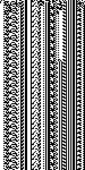
Figure D.1: Computer simulation of the Stag Hunt, a modified Arthur-Packard- Rogers cellular game model, with $75$ cells, and $150$ generations per round. Program cg2.pas, random seed $824709136$, generation 1. In this program, all initial strategies are depth $1$, but strategies of depth up to $3$ may be introduced as the system evolves.

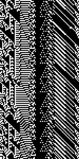
Figure D.2: The same program, parameters, and seed as above, generation $27$. Notice the rightward-moving waves of cooperative behavior, in the right part of the display. Here some zones exhibit cellular automaton-like triangular patterns.

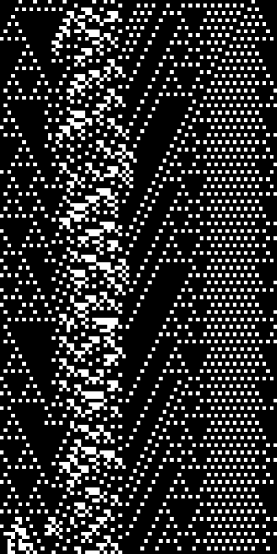
Figure D.3: Generation $139$ of this run. Cellular automaton-like triangles predominate in this figure.

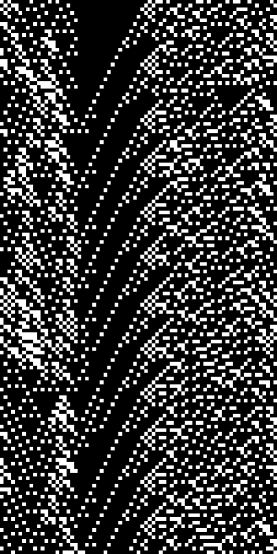
Figure D.4: Generation $165$. There are now leftward-moving waves of cooperative behavior, in the middle of the display.

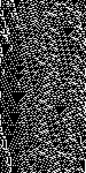
Figure D.5: Generation $305.$

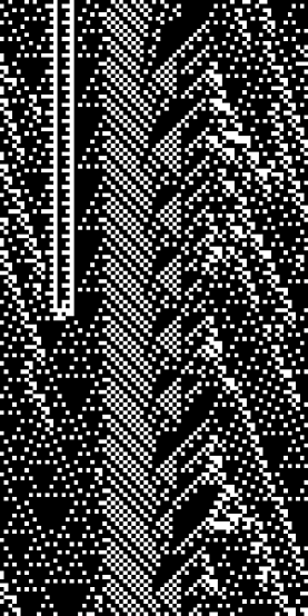
Figure D.6: Generation $483$. Cellular automaton-like triangles appear again.

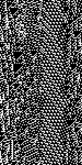
Figure D.7: Generation $560$. Move behavior does not appear to have changed much in many generations.

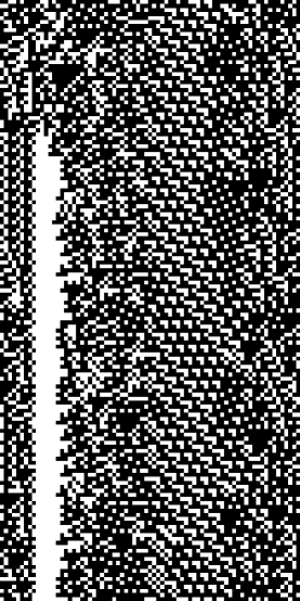
Figure D.8: Generation $561$. An all-cooperate zone appears. The next three figures show the rapid growth of this zone.

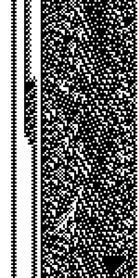
Figure D.9: Generation $612$.

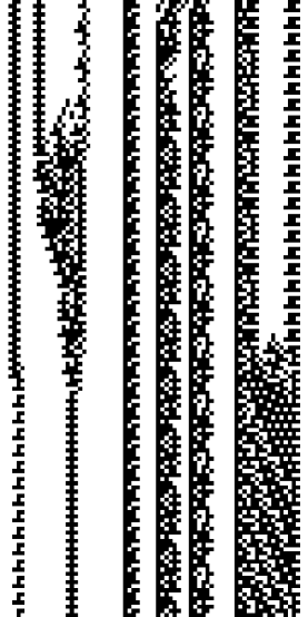
Figure D.10: Generation $658$.

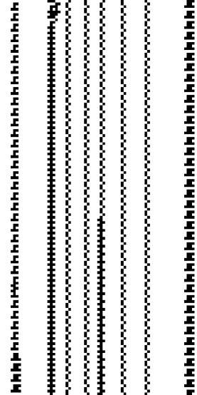
Figure D.11: Generation $662$. The all-cooperate zone has almost completely taken over the ring.

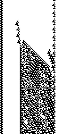
Figure D.12: Generation $930$. Large all-cooperate zones have predominated in the past several hundred generations. However, at this point, a perturbation in strategy – that is, an unexpected defect move – can set off many defect moves in other cells.

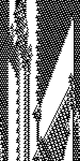
Figure D.13: Generation $982$. Recovery of an all-cooperate zone.

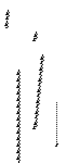
Figure D.14: Generation $1262$. At this point, perturbations do not set off much defecting behavior in other cells. That is, strategies are no longer, “Cooperate unless there are defectors in the neighborhood,” but, “Cooperate, whatever happens.”

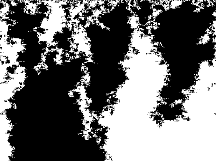
Figure D.15: Computer simulation of a one-round cellular game, the Cloud Process, on a ring of $640$ cells. The table for this game is: $G(BBB)=G(WWW)=0.27$, $G(BBW)=G(BWB)=G(BWW)=G(WBB)=G(WBW)=G(WWB)=0.53$. Program cloud.pas, random seed $118950941$. Initial conditions were chosen with the aid of a pseudorandom number generator.

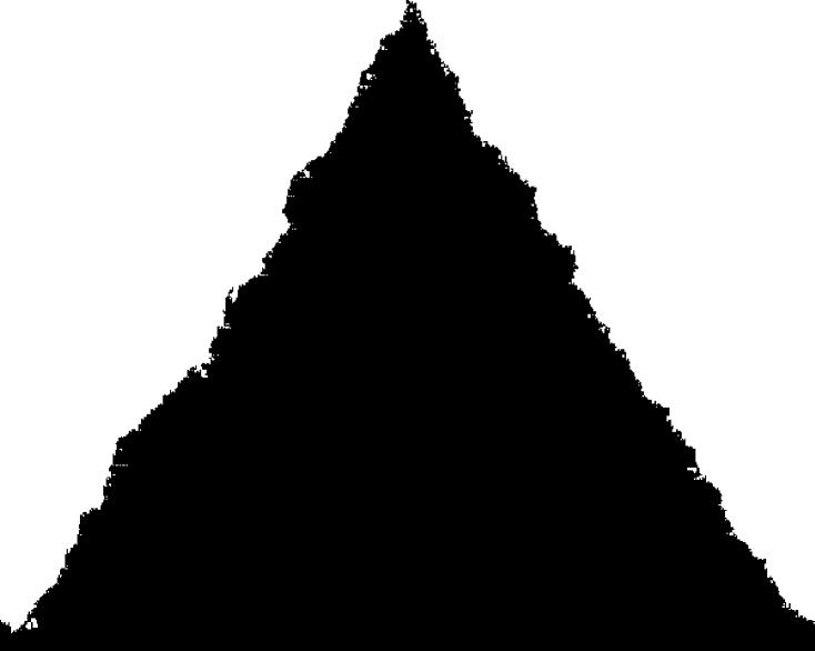
Figure D.16: Computer simulation of a one-round Prisoner’s Dilemma game on a ring of $600$ cells. Initially, two defectors are placed side-by- side; all other cells are cooperators. (Black indicates defecting cells, and white, cooperating.) Program prisoner.pas, random seed $424479774$. Note that the rate of expansion of the black domain appears roughly similar on each side, thus suggesting an informal estimate of the expected rate.

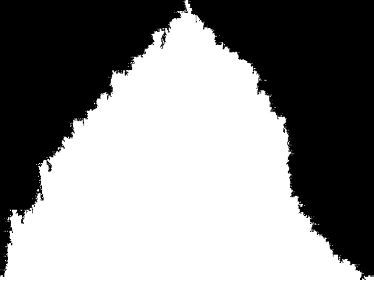
Figure D.17: Computer simulation of a zero-depth, one round per generation Stag Hunt game on a ring of $600$ cells. Initially, four cooperators are placed contiguously; all other cells are defectors. Program stag.pas, random seed $941165838$. Note that, in this case, the rate of expansion of the white domain appears to vary considerably.

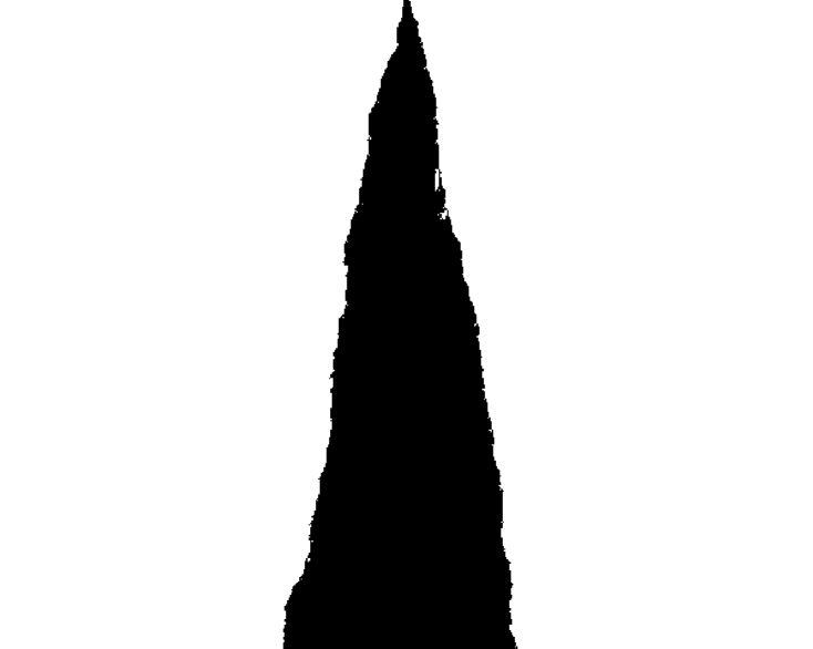
Figure D.18: Computer simulation of a zero-depth, one round per generation Stag Hunt game on a ring of $600$ cells. Initially, four defectors are placed contiguously; all other cells are cooperators. Program stag2.pas, random seed $90049811$.

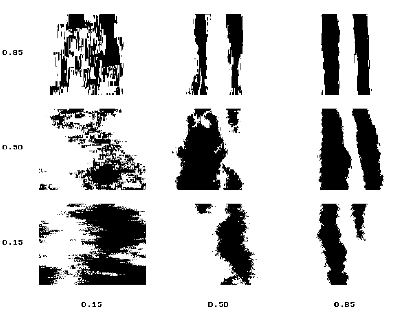
Figure D.19: Join/mix processes with various parameters. Each process is run on a circular lattice of $165$ cells for $125$ generations. Initially, all cells are white except for cells $48$ through $70$, and $95$ through $117$. The numbers at the bottom show the values of $p_{1}$; and those on the left show the values of $p_{2}$. That is, both $p_{1}$ and $p_{2}$ are set at $0.15$, $0.50$, and $0.85$. The program used is square.pas, seed $252644401$.

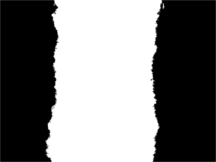
Figure D.20: Computer simulation of the Join or Die Process on a ring of $640$ cells. Initial conditions are black for cells $0$ through $127$, and $512$ through $639$, and white for cells $128$ through $511$. Program jd.pas, random seed $274535429$.

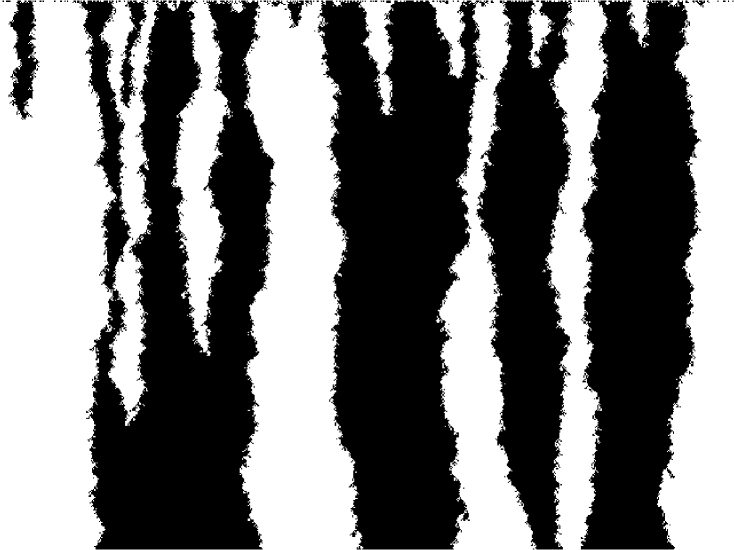
Figure D.21: Computer simulation of the Join or Die Process. Initial conditions were chosen with the aid of a pseudorandom number generator, so each cell is equally likely to be black or white. Random seed $705238026$ is used; and the same program, and ring size, as in the preceding figure.

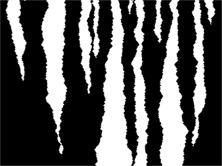
Figure D.22: The annihilating particle model, on a ring of $640$ cells, which initially contains $28$ particles. Program apm.pas, seed $269093635$. Each particle executes a symmetric random walk, having a $50\%$ probability of going either left or right in each generation.

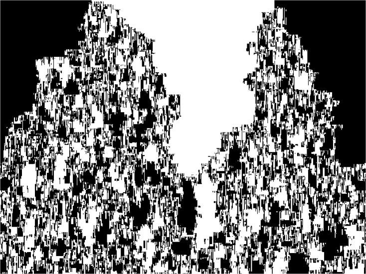
Figure D.23: Computer simulation of the Mixing Process on a ring of $640$ cells. Initial conditions are black for cells $0$ through $127$, and $512$ through $639$, and white for cells $128$ through $511$. Program mix.pas, random seed $912200719$.

Vita

Lenore E. Levine was born in Brooklyn, New York. She graduated from Regents College with a B.S., concentration in Computer Science, in May 1988, and from the University of Illinois with a M.S. in Mathematics in January 1991. From 1984 to 1988, she worked as a software engineer for DPI Services, Inc., in San Jose, California. She entered the Graduate College of the University of Illinois at Urbana-Champaign in August 1988. While at Illinois, she held a fellowship and a teaching assistantship.

References

- [1] Axelrod, R., The Evolution of Cooperation, (Basic Books, Inc., 1984).
- [2] Berger, R., “The Undecidability of the Domino Problem,” Mem. Amer. Math. Soc., 66 (1966).
- [3] Cowan, R., and Miller, J. H., The Santa Fe Institute, “Life on a Lattice: The Nature of Equilibria in Spatially Overlapping Games,” unpublished.
- [4] Cowan, R. and Miller, J. H., “Economic Life on a Lattice: Some Game Theoretic Results,” Santa Fe Institute Working Paper 90-10, 1990.
- [5] Erdős, P., and Ney, P., “Some Problems on Random Intervals and Annihilating Particles,” The Annals of Probability, 2:5 (1974) 828-839.
- [6] Goldberg, D. E., Genetic Algorithms in Search, Optimization, and Machine Learning, (Addison-Wesley, 1989).
- [7] Langton, C. G., Artificial Life, (Addison-Wesley, 1989).
- [8] Levy, Steven, Artificial Life, (Pantheon, 1992).
- [9] Luce, R. D., and Raffia, H., Games and Decisions, (Wiley, 1957; Dover, 1985).
- [10] Matsuo, K., and Adachi, N., “Metastable Antagonistic Equilibrium and Stable Cooperative Equilibrium in Distributed Prisoner’s Dilemma Game,” Proceedings of the International Symposium on Systems Research, Informatics and Cybernetics, Baden-Baden, 1989.
- [11] Matsuo, K., and Adachi, N., “How to Attain to Cooperative Society in Game World: The Choice of Selection Rules,” preprint, The International Institute for Advanced Study of Social Information Science, Fujitsu Laboratories, Ltd., Japan.
- [12] Matsuo, K., and Adachi, N., “Ecological Dynamics under Different Selection Rules in Distributed and Iterated Prisoner’s Dilemma Game,” preprint, The International Institute for Advanced Study of Social Information Science, Fujitsu Laboratories, Ltd., Japan.
- [13] Miller, J. H., “The Evolution of Automata in the Repeated Prisoner’s Dilemma,” Essay in Ph.D. Dissertation, the University of Michigan, 1988.
- [14] Mitchell, M., Hraber, P. T., and Crutchfield, J. P., “Revisiting the Edge of Chaos: Evolving Cellular Automata to Perform Computations,” Santa Fe Institute Working Paper 93-03-014, 1993.
- [15] Nowak, M. A., and May, R. M., “Evolutionary Games and Spatial Chaos,” Nature, 359 (1992) 826.
- [16] Packard, N., The Prediction Company, personal communication (1993).
- [17] Packard, N., “Adaptation Toward the Edge of Chaos.” In Dynamic Patterns in Complex Systems, pages 293-301, (World Scientific, Singapore, 1988).
- [18] Poundstone, W., The Prisoner’s Dilemma, (Doubleday, 1993).
- [19] Robinson, R. M., “Undecidability and Nonperiodicity for Tilings of the Plane,” Inventiones Mathematicae, 12 (1971) ,177-209.
- [20] Rogers, K. C., “Cellular Automata Simulations Exhibiting an Evolutionary Increase in Complexity,” Master’s Thesis, the University of Illinois, Department of Electrical Engineering, (1990).
- [21] Rudin, W., Real and Complex Analysis, 3rd ed, (McGraw-Hill, 1987).
- [22] Waldrop, M. M., Complexity, (Simon and Schuster, 1992).
- [23] Waterman, M. S., “Some Applications of Information Theory to Cellular Automata,” Physica 10D, (1984), 45-51.
- [24] Wolfram, S., “Statistical Mechanics of Cellular Automata,” Review of Modern Physics, 55 (1983), 601-644.
- [25] Wolfram, S., “Universality and Complexity in Cellular Automata,” Physica 10D, (1984), 1-35.
Vita