AutoFed: Manual-Free Federated Traffic Prediction via Personalized Prompt

Abstract

Accurate traffic prediction is essential for Intelligent Transportation Systems, including ride-hailing, urban road planning, and vehicle fleet management. However, due to significant privacy concerns surrounding traffic data, most existing methods rely on local training, resulting in data silos and limited knowledge sharing. Federated Learning (FL) offers an efficient solution through privacy-preserving collaborative training; however, standard FL struggles with the non-independent and identically distributed (non-IID) problem among clients. This challenge has led to the emergence of Personalized Federated Learning (PFL) as a promising paradigm. Nevertheless, current PFL frameworks require further adaptation for traffic prediction tasks, such as specialized graph feature engineering, data processing, and network architecture design. A notable limitation of many prior studies is their reliance on hyper-parameter optimization across datasets—information that is often unavailable in real-world scenarios—thus impeding practical deployment. To address this challenge, we propose AutoFed, a novel PFL framework for traffic prediction that eliminates the need for manual hyper-parameter tuning. Inspired by prompt learning, AutoFed introduces a federated representor that employs a client-aligned adapter to distill local data into a compact, globally shared prompt matrix. This prompt then conditions a personalized predictor, allowing each client to benefit from cross-client knowledge while maintaining local specificity. Extensive experiments on real-world datasets demonstrate that AutoFed consistently achieves superior performance across diverse scenarios. The code of this paper is provided at https://github.com/RS2002/AutoFed.

1 Introduction

Traffic Prediction (TP) is a cornerstone of modern Intelligent Transportation Systems (ITS), enabling critical applications such as real-time ride-hailing dispatch, dynamic pricing, urban infrastructure planning, and congestion management [tedjopurnomo2020survey]. However, the development of robust TP models faces a fundamental challenge: although traffic data is abundant, it is also highly sensitive and fragmented [zhang2024survey]. Stringent privacy regulations and commercial interests often result in this data being confined to isolated silos maintained by various municipal authorities (e.g., agencies in different jurisdictions) or private companies (e.g., Uber, Lyft). As a result, centralized training on aggregated datasets is generally infeasible, and most practical solutions must rely on local training with limited data. This siloed approach leads to poor generalization and an inability to capture broader, transferable patterns essential for effective traffic prediction.

Federated Learning (FL) has emerged as a promising paradigm for collaboratively training models without sharing raw data, thereby preserving privacy [zhang2021survey]. However, conventional FL algorithms such as FedAvg [fedavg] are built on the assumption that client data are Independent and Identically Distributed (IID)—an assumption that is rarely satisfied in the context of traffic prediction. In reality, traffic patterns exhibit significant heterogeneity (non-IID) across different regions, driven by variations in urban layout, population density, and economic activity. Training a single global model on such non-IID data can lead to client drift and suboptimal performance for all participants. Personalized Federated Learning (PFL) addresses this challenge by allowing clients to learn customized models while still leveraging collective knowledge from the federation [tan2022towards]. As a result, PFL has become a particularly promising framework for achieving realistic, privacy-preserving traffic prediction.

Nevertheless, existing PFL frameworks are not directly suited for the unique challenges of TP. Compared to standard time series prediction tasks, TP faces significant challenges, including complex spatiotemporal dependencies, non-stationary fluctuations, and numerous external features [aouedi2025deep]. This necessitates the adaptation of standard PFL frameworks to meet the specific demands of TP tasks, where traditional methods often fail to incorporate domain-specific needs. Unfortunately, these adaptation processes frequently rely on complex manual efforts, such as intricate graph construction [shang2025security; shang2025II; yuan2022fedstn] or hyper-parameter tuning [hu2024fedgcn; zhou2025fedtps; zhou2024traffic]. For instance, the filter method and pattern amount in [hu2024fedgcn; zhou2025fedtps] can result in performance variations of over 5% based solely on parameter adjustments mentioned in their papers. However, optimal settings can vary significantly between datasets, and a single configuration can lead to substantial performance variability. The setting process is often contingent upon prior knowledge of the dataset and client configurations or expert insights, which can be challenging to obtain in practice, creating significant barriers to robust and scalable deployment.

To address these challenges, we propose a novel PFL framework for TP, named AutoFed, which eliminates the need for manual adaptation efforts. AutoFed comprises two key components: a Personalized Predictor (PP) that adapts to local data distributions and a Federated Representor (FR) that shares and provides global common knowledge. For the PP, we utilize the Adaptive Graph Convolutional Recurrent Network (AGCRN) [bai2020adaptive], which can learn the adjacency matrix adaptively, thus removing the need for manual design tailored to different clients. Unlike conventional FL approaches that rely on model parameter aggregation, the FR is inspired by prompt learning. Specifically, it first compresses local input data through the Auto-Encoder (AE) denoiser and AGCRN encoder to capture refined local features [lee2021noise]. Then, following the principle of FedBN [li2021fedbn], the FR leverages shared linear layers of the Multi-Layer Perceptron (MLP) to align these local features into a unified global representation across clients, while retaining distinct batch normalization layers for each client to preserve personalized statistical characteristics. This generates a personalized prompt for the PP while adapting to non-IID data distributions. This design enables AutoFed to create adaptive and personalized global prompt representations, eliminating the need for manual hyper-parameter tuning and enhancing the framework’s robustness and generalization ability. Compared to previous methods such as [hu2024fedgcn; zhou2025fedtps; zhou2024traffic], our approach demonstrates superior performance across a range of real-world TP datasets.

2 Related Work

2.1 Traffic Prediction

Serving as a key component of ITS, TP encompasses various tasks such as travel demand prediction, traffic flow prediction, and travel time prediction. Early research treated each traffic node as an independent entity, framing TP as a general time series prediction task. Many methods were developed based on conventional single-dimensional time series approaches, including statistical methods [liu2011discovering], cluster-based pattern matching [zhang2013improved], and neural networks [yang2019traffic]. However, these approaches often overlook the spatial relationships among traffic nodes. For instance, when a traffic jam occurs in one area, neighboring regions are likely to experience increased traffic flow as well. Subsequently, most approaches adopted a paradigm that first extracts spatial features within each time frame and then employs time series networks for prediction. For example, [liu2011discovering; asif2013spatiotemporal; ke2017short] proposed a CNN-LSTM network for traffic flow prediction. However, CNN-based spatial extraction struggles to adequately represent the non-Euclidean nature of traffic networks, resulting in challenges in accurately learning robust spatial features [zhou2024traffic; zhou2025fedtps]. Recently, Graph Neural Networks (GNNs) have emerged as a promising solution, effectively capturing the relationships among nodes in traffic networks. An example is the AGCRN [bai2020adaptive], which uses a GCN-LSTM structure and employs adaptive adjacency matrices to capture spatial dependencies, allowing for end-to-end learning. Additionally, STWave [fang2023spatio] introduced a novel decoupling approach to separate traffic data into stationary and non-stationary components, utilizing both temporal and spatial attention methods to capture relationships accurately.

Despite these advancements, most of these methods rely on centralized training, neglecting the privacy considerations inherent in traffic data, which are increasingly recognized by data privacy regulations such as the General Data Protection Regulation (GDPR) and the California Consumer Privacy Act (CCPA). Recently, some research has begun to focus on FL-based paradigms to address privacy concerns. For instance, Shang et al. [shang2025security; shang2025II] proposed both horizontal and vertical methods based on FedAvg [fedavg], in which a carefully designed traffic graph efficiently captures the relationships among traffic nodes. Additionally, Hu et al. [hu2024fedgcn] introduced FedGCN, which considers the relationship between graph nodes and external factors through a novel MendGCN module. In the realm of PFL methods, Zhou et al. [zhou2024traffic; zhou2025fedtps] developed FedTPS, which utilizes a traffic pattern repository to share knowledge among clients. However, most of these methods depend on meticulous manual feature design and hyper-parameter optimization tailored to specific clients or datasets, which hinders their efficient application and adaptation to distinct contexts.

2.2 Federated Learning

In recent years, FL has been widely applied in high-privacy and resource-limited scenarios [cai2025feedsign], including medical recognition [pfitzner2021federated], traffic prediction [shang2025explainable], and autonomous driving [kou2025fast]. However, standard FL methods like FedAvg rely on the assumption of IID data among clients, which is not always feasible in practice. According to [pei2024review], solutions for non-IID data distributions can be categorized into three types: data-based, framework-based, and model-based methods. Among these, PFL, as a model-based approach, shows promising performance. In PFL, clients share only portions of the model to leverage common knowledge while retaining personalized parameters or structures to adapt to local data distributions.

Starting with FedPer [fedper], different clients share upstream layers for robust feature extraction while keeping personalized downstream layers for final output, which is also a well-recognized paradigm in the theory of transfer learning [zhuang2020comprehensive]. Following this, various methods have introduced innovative technologies such as clustering [chang2025dual], where clients within a single cluster share data distribution similarities; meta-learning [fallah2020personalized], which aims to find a suitable starting point for all clients; and hyper-networks [scott2024pefll], which directly output personalized network parameters with a high capacity for expansion to new clients. Moreover, PFL can be effectively utilized in scenarios where different clients have varying model structures, as it allows for the aggregation of common sub-networks. This flexibility is particularly advantageous when clients possess different computational resources for varying model scales. As mentioned in the introduction, due to the unique challenges in TP, it is essential to adapt these methods for specific tasks. However, this adaptation still encounters the challenges faced by conventional TP models discussed in the previous subsection.

2.3 Prompt Learning

Recently, the success of Large Language Models (LLMs) [chen2026overview] has led to the effective application and adaptation of various related technologies, such as Masked Language Model (MLM) pre-training [zhao2025csi], Retrieval-Augmented Generation (RAG) [hanretrieval], and LLMs themselves [jin2024time], in time series analysis. Among these technologies, prompt learning is recognized for its efficiency and ease of implementation. In the context of LLMs, prompts play a crucial role in directly influencing the subsequent output decoding, a concept well-established since the development of T5 [raffel2020exploring]. Subsequently, prompt tuning has emerged as a promising solution for enhancing or fine-tuning models with low cost by utilizing learnable prompt tokens [li2025survey].

In the field of time series analysis, most research has concentrated on designing prompts to adapt pre-trained LLMs or their architectures for specific tasks [caotempo; xue2023promptcast]. For example, [huang2025timedp; zhou2024traffic; zhou2025fedtps] employ learnable prototypes (or patterns) as guiding prompts for the decoding process. However, the number of prototypes can significantly impact model performance, and the optimal quantity varies across datasets [zhou2024traffic; zhou2025fedtps]. In contrast, this paper proposes a neural network-based prompt generator, eliminating the need for prototypes. Furthermore, while some graph-based works have also introduced prompt learning [li2024graph], their focus is primarily on designing spatial prompt representations, which differs from our emphasis on the temporal dimension.

3 Methodology

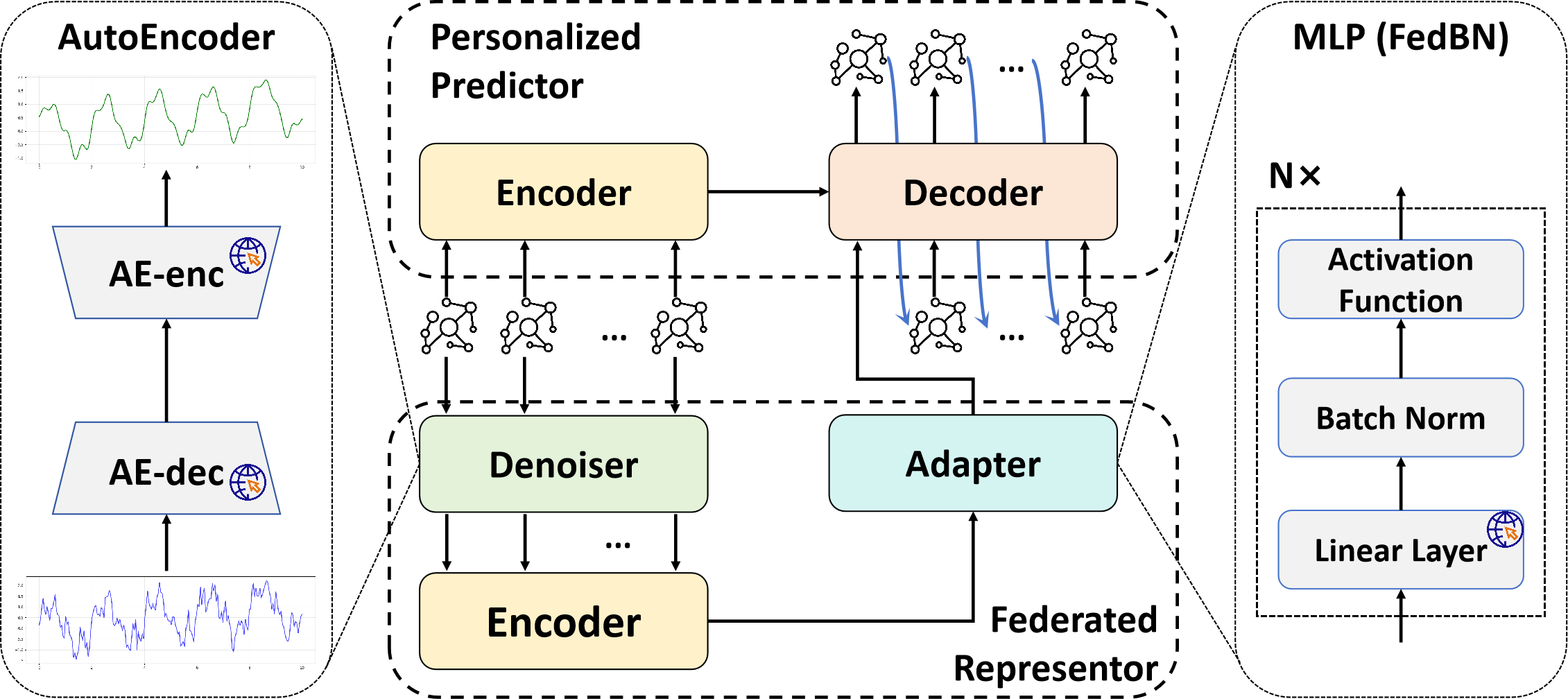
Figure 1: Network Architecture: The network consists of the PP and FR. PP utilizes a graph time series network with an encoder-decoder structure. FR employs an AE-based denoiser for robust feature extraction, a graph time series encoder for feature compression, and an client-aligned adapter for transferring local representations to global representations, providing a guided prompt matrix for the decoder in PP. In the figure, only the modules with the “earth" icon are shared among clients.

3.1 Problem Setup

In this paper, we study the federated TP task, which involves $m$ clients $\mathcal{C}=\{C_{1},C_{2},\ldots,C_{m}\}$ with non-IID data and a centralized server $S$. For each region $i\in\{1,\ldots,n\}$, the transportation network can be represented as $G_{i}=(V_{i},E_{i})$, where $V_{i}$ and $E_{i}$ denote the nodes and edges, respectively. Additionally, $A_{i}\in\mathbb{R}^{|V_{i}|,|V_{i}|}$ is the weighted adjacency matrix, representing the relationship (e.g. spatial, similarity, and dependencies) among traffic nodes, where and $|\cdot|$ represents the size of set. Specifically, each client possesses a private dataset $D_{i}=\{X_{i},Y_{i}\}$, where $X_{i}\in\mathbb{R}^{N_{i},\mathcal{T},|V_{i}|,H}$ represents the historical traffic features, and $Y_{i}\in\mathbb{R}^{N_{i},\mathscr{T},|V_{i}|}$ is the ground truth for future demand. Specifically, $N_{i}$ denotes the sample size for client $i$, $\mathcal{T}$ and $\mathscr{T}$ are the lengths of the historical information sequence and the future horizon to be predicted, respectively, and $H$ is the feature dimension.

Specifically, we consider a PFL scenario, where the network of each client $i$ at round $m$ can be expressed as $\text{f}(\cdot;\theta_{i}^{m},\Theta^{m})$, where $\theta_{i}^{m}$ represents the private part of the network parameters of client $i$, which learns the personalized aspects of the data in their own data distribution, while $\Theta^{m}$ denotes the shared part of the network parameters, which learns a global general representation for all clients. Consequently, the target of PFL is defined as:

$$\arg\min_{\theta_{1},\theta_{2},\ldots,\theta_{n},\Theta}\sum_{i=1}^{n}\frac{|V_{i}|}{\sum_{i=1}^{n}|V_{i}|}\text{L}(\text{f}(X_{i};\theta_{i},\Theta),Y_{i})\ ,$$ (1)

where $\text{L}(\cdot,\cdot)$ is the loss function.

3.2 Method Overview

The network structure is depicted in Fig. 1, comprising two main components: the Personalized Predictor (PP) and the Federated Representor (FR). The PP utilizes an encoder-decoder-based graph time series network that is trained locally, allowing it to adapt to local data distributions. During inference, the encoder receives historical data $x\in\mathbb{R}^{\mathcal{T},n,H}$ as input, while the decoder predicts future traffic data $\hat{y}\in\mathbb{R}^{\mathscr{T},n}$ in an Auto-Regressive (AR) manner. For client $i$, the input $x$ is derived from its dataset $X_{i}$, where $n$ represents the number of nodes ($|V_{i}|$). Specifically, the FR generates a prompt matrix $p_{g}\in\mathbb{R}^{n,h}$ based on the input $x$ (where $h$ is the hidden dimension), which serves as a prefix token for the decoder. This design is motivated by the intuition that different clients may share similar traffic patterns [zhou2024traffic; zhou2025fedtps], allowing the prefix prompt to convey pertinent pattern information from the input $x$ and guide the decoding process. During training, the parameters of the FR are partially shared among clients, facilitating the learning of a global common traffic pattern representation. Simultaneously, personalized components are also employed to adapt to local data distributions like PP.

3.3 Personalized Predictor

Although our framework is ultimately dependent on a graph time series model, we recommend utilizing methods with adaptive graph structures, such as the AGCRN [bai2020adaptive], which is also employed in the experiments of this paper. This recommendation is based on the following considerations. Currently, most traffic prediction models rely on manually designed graphs [shang2025security; shang2025explainable]. While these approaches yield promising results, constructing such graphs is time-consuming and requires careful consideration of multiple factors, including spatial connections, distance relationships, and node similarities. Furthermore, the effectiveness of each graph feature may vary across different regions or datasets. In contrast, AGCRN adapts the graph structure through a learnable parameter, $E\in\mathbb{R}^{n,h}$. The AGCRN process can be represented as:

$$\tilde{A} =\text{Softmax}(\text{ReLU}(EE^{T}))\ ,$$ (2)

$$u_{t} =\sigma(\operatorname{GCN}_{u}(x_{t},H_{t-1},\tilde{A}))\ ,$$

$$r_{t} =\sigma(\operatorname{GCN}_{r}(x_{t},H_{t-1},\tilde{A}))\ ,$$

$$C_{t} =\tanh(\operatorname{GCN}_{C}(x_{t},(r_{t}\odot H_{t-1}),\tilde{A}))\ ,$$

$$H_{t} =u_{t}\odot H_{t-1}+(1-u_{t})\odot C_{t}\ ,$$

where the matrix $\tilde{A}\in\mathbb{R}^{n,n}$ is the adaptive adjacency matrix, $x_{t}\in\mathbb{R}^{n,H}$ represents the input $x$ at frame $t$ (i.e. $x=\{x_{1},x_{2},\ldots,x_{\mathcal{T}}\}$), and $u_{t},r_{t},C_{t},H_{t-1}\in\mathbb{R}^{n,h}$ represent the update gate, reset gate, candidate state, and previous hidden state of the GRU at frame $t$, respectively. Specifically, we employ the same AGCRN structure both the encoder and decoder in the PP.

3.4 Federated Representor

As shown in Fig. 1, the FR consists of three components: an Auto-Encoder (AE) denoiser for robust feature extraction, a graph time series encoder for further information extraction and compression, and a client-aligned adapter to transfer the local feature representation to a global common feature prompt, which serves as guidance for the PP.

• Auto-Encoder Denoiser: The goal of the FR is to generate a guiding prompt that captures the traffic pattern information, which necessitates a focus on stable features while ignoring random noise. While some previous works have utilized low-pass filters [zhou2024traffic; zhou2025fedtps; fang2023spatio], selecting the appropriate filtering method and its hyper-parameters can be challenging, directly affecting model performance [zhou2024traffic; zhou2025fedtps]. Additionally, these methods rely on the assumption that low-frequency components contain more stable patterns, whereas high-frequency components contain more noise. However, the specific threshold between these components is often unclear. To address these issues, we propose using an AE-based denoiser that can learn stable patterns autonomously. This approach has proven effective in various fields, including signal processing [nguyen2025robust] and image denoising [lee2021noise]. The denoising process can be represented as:

  $$p =\text{AE-enc}(x)\ ,$$ (3)

  $$\hat{x} =\text{AE-dec}(p)\ ,$$

  where the AE encoder compresses the original input sequence $x\in\mathbb{R}^{\mathcal{T},n,H}$ into a feature space $p\in\mathbb{R}^{\mathcal{T},n,h}$, and the AE decoder attempts to recover it back to the original input $\hat{x}\in\mathbb{R}^{\mathcal{T},n,H}$. Since time series data predominantly consists of regular patterns and irregular noise, recovering the noise element can be challenging, allowing the AE to effectively perform denoising. Since denoising is similar across different nodes, we choose to share this module among clients. Compared to the recovered sequence $\hat{x}$, the hidden feature $p$ includes more dense information, which we utilize for subsequent computations. The recovered sequence $\hat{x}$ be used solely for calculating the AE loss during training.

• Graph Time Series Encoder: Even though the AE denoiser provides robust stable features, it can be difficult to use the long-sequence $p$ as a prompt for the PP. Therefore, we propose utilizing a graph time series encoder to compress $p$ while extracting additional information. Specifically, we adopt the same encoder structure as the PP, compressing the feature $p$ into a single vector $p_{l}\in\mathbb{R}^{n,h}$, referred to as the local feature. Given the differing graph structures and data distributions among clients, we opt for a personalized encoder for each client.

• Client-Aligned Adapter: To facilitate knowledge sharing among clients, we introduce a client-aligned adapter that transfers the local traffic pattern representation $p_{l}$ to a global representation $p_{g}\in\mathbb{R}^{n,h}$. For this process, we utilize a shared MLP. Specifically, we employ the FedBN [li2021fedbn] strategy to tackle the challenges posed by non-IID data, which persists in the local feature space $p_{l}$. In detail, the parameters of the linear layers are shared among clients, while the batch normalization layers remain distinct, retaining their statistical information, such as the average values and standard deviations, along with the rescaling parameters.

  To summarize, the full process of the PP can be expressed as follows:

  $$H_{\mathcal{T}} =\text{Encoder}(x;\mathbf{0})\ ,$$ (4)

  $$z =\text{Decoder}(p_{g};H_{\mathcal{T}})\ ,$$

  $$\hat{y} =\text{MLP}(z)\ ,$$

  where $\mathbf{0}$ represents a zero matrix that serves as the initial hidden state for the encoder, $p_{g}$ is the first input token for the decoder, $H_{\mathcal{T}}$ is the final hidden state of the encoder, which serves as the initial hidden state for the decoder, the variable $z\in\mathbb{R}^{\mathscr{T},n,h}$ is the output of the decoder, and an additional MLP $(\mathbb{R}^{h}\rightarrow\mathbb{R})$ maps $z$ to the final prediction result $\hat{y}\in\mathbb{R}^{\mathscr{T},n}$. It is important to note that the intermediate output $z$ is necessary because the output dimension of each token in the decoder must match that of the first prompt token $p_{g}$, due to its AR nature. Note that although the encoder and decoder have the same structure, the inputs ($x$ and $p_{g}$) have different dimensions. This is because the decoder follows the AR paradigm, while the encoder processes the full input sequence.

3.5 Training Process

In considering the training process, we first define the loss function, which consists of two parts: the regression loss of the AE-denoiser and the regression loss of the PP. In this paper, we choose the Mean Absolute Error (MAE) as the loss function. For each client $i$, the two loss functions can be represented as:

$$L^{ae}_{i} =\mathbf{E}_{x\in X_{i}}||x-\hat{x}||_{1}\ ,$$ (5)

$$L^{pre}_{i} =\mathbf{E}_{y\in Y_{i}}||y-\hat{y}||_{1}\ ,$$

where $||\cdot||_{1}$ denotes the $L_{1}$ norm. The overall loss function for client $i$ is then defined as:

$$L_{i} =L^{pre}_{i}+\alpha L^{ae}_{i}\ ,$$ (6)

$$\alpha =\frac{L^{ae}_{i}}{L^{pre}_{i}}\ ,$$

where $\alpha$ is an adaptive hyper-parameter, inspired by [zhao2025let]. This approach allows the training process for denoising and prediction to adaptively balance: when the denoiser has a high error, the prompt matrix may not be effective, making a large weight for the prediction loss less meaningful since the prompt matrix will change thereafter. Thus, a higher weight for the denoising loss is warranted. This relationship is vice versa as well. The detailed training process follows the conventional PFL paradigm, as shown in Appendix A.

4 Experiment

Table 1: Model Performance on TDP Task: The best results are highlighted in bold, while the second-best results are indicated with underlining. This notation is consistent throughout the following tables.

Type	Method	Uber (S0)				Lyft (S0)
		MAE	RMSE	MSE	MAPE/%	MAE	RMSE	MSE	MAPE/%
Local Training		3.64	6.12	37.54	39.36	1.97	3.12	9.76	50.41
FL	FedAvg [fedavg]	3.50	5.92	35.14	40.51	1.88	3.00	9.00	48.91
	FedProx [fedprox]	3.55	5.92	35.14	39.45	1.83	2.87	8.25	50.05
PFL	FedPer [fedper]	3.51	5.87	34.61	41.72	1.87	2.92	8.55	50.97
	pFedMe [pfedme]	3.61	6.13	37.70	40.00	1.96	3.10	9.61	50.72
TrafficFL	FedTPS [zhou2024traffic; zhou2025fedtps]	3.47	5.85	34.24	40.35	1.88	2.96	8.74	50.71
	FedGCN [hu2024fedgcn]	3.33	5.65	32.06	38.57	1.82	2.88	8.29	48.63
Ours	AutoFed	3.35	5.65	32.01	38.95	1.82	2.88	8.29	48.55
	w/o AE	3.53	5.94	35.30	39.19	1.89	2.99	8.95	48.74
	w/o FedBN	3.52	5.90	34.83	40.33	1.96	3.13	9.81	48.74
Type	Method	Uber (S1)				Lyft (S2)
		MAE	RMSE	MSE	MAPE/%	MAE	RMSE	MSE	MAPE/%
Local Training		3.40	5.35	32.72	39.60	1.87	2.85	8.56	50.02
FL	FedAvg [fedavg]	3.55	5.68	37.30	40.17	1.89	2.88	8.75	51.05
	FedProx [fedprox]	3.57	5.73	38.37	39.91	1.89	2.89	8.80	51.44
PFL	FedPer [fedper]	3.59	5.65	36.46	40.49	1.89	2.90	8.81	51.29
	pFedMe [pfedme]	3.39	5.33	32.31	40.12	1.89	2.89	8.83	50.37
TrafficFL	FedTPS [zhou2024traffic; zhou2025fedtps]	3.46	5.44	33.80	39.25	1.85	2.83	8.44	50.25
	FedGCN [hu2024fedgcn]	3.46	5.48	33.96	39.61	1.88	2.87	8.69	49.87
Ours	AutoFed	3.36	5.25	31.38	38.82	1.81	2.74	8.01	50.12
	w/o AE	3.40	5.32	32.31	39.39	1.85	2.84	8.61	49.52
	w/o FedBN	3.37	5.29	31.75	39.05	1.85	2.83	8.42	50.46
Type	Method	Uber (S3)				Lyft (S3)
		MAE	RMSE	MSE	MAPE/%	MAE	RMSE	MSE	MAPE/%
Local Training		3.40	5.35	32.72	39.60	1.87	2.85	8.56	50.02
FL	FedAvg [fedavg]	3.63	5.90	41.49	40.36	1.86	2.86	8.62	49.45
	FedProx [fedprox]	3.57	5.74	39.27	40.56	1.87	2.85	8.60	49.81
PFL	FedPer [fedper]	3.67	5.79	38.32	40.62	1.92	2.94	9.13	51.85
	pFedMe [pfedme]	3.41	5.38	33.10	39.84	1.86	2.84	8.51	50.48
TrafficFL	FedTPS [zhou2024traffic; zhou2025fedtps]	3.42	5.42	33.66	39.38	1.85	2.84	8.52	50.09
	FedGCN [hu2024fedgcn]	3.50	5.56	34.93	39.66	1.91	2.94	9.08	50.43
Ours	AutoFed	3.32	5.19	30.63	39.35	1.83	2.79	8.22	50.00
	w/o AE	3.41	5.35	32.74	39.21	1.84	2.80	8.40	49.50
	w/o FedBN	3.38	5.34	32.56	39.38	1.85	2.83	8.43	50.73

Table 2: Model Performance on TFP Task: Results from comparative experiments are sourced from [zhou2024traffic; zhou2025fedtps; hu2024fedgcn]. The MAPE for FedGCN [hu2024fedgcn] is not provided in their paper. Additionally, we omit the MSE metric for this task, as it is not reported in all studies.

Method PEMS03 [pems] PEMS04 [pems] PEMS07 [pems] PEMS08 [pems] MAE RMSE MAPE/% MAE RMSE MAPE/% MAE RMSE MAPE/% MAE RMSE MAPE/% Local Training 15.86 26.31 16.65 20.22 31.79 13.89 22.14 35.72 10.66 16.11 25.41 10.86 FedAvg [fedavg] 16.55 26.61 22.90 20.23 31.87 14.42 24.29 37.12 11.51 16.29 25.56 11.16 FedProx [fedprox] 16.35 26.52 21.13 20.73 32.31 14.66 25.10 38.12 12.41 16.51 25.44 11.87 FedPer [fedper] 15.56 26.29 15.43 19.72 31.42 12.99 24.56 37.48 11.68 16.08 25.40 10.24 pFedMe [pfedme] 15.48 26.44 15.13 19.60 31.21 12.88 22.67 35.55 9.58 15.96 24.98 10.14 FedTPS [zhou2024traffic; zhou2025fedtps] 15.05 25.94 14.70 19.46 31.18 12.67 21.74 34.57 9.16 15.81 24.91 10.28 FedGCN [hu2024fedgcn] 15.87 23.78 – 20.46 30.75 – 20.50 35.22 – 16.56 24.91 – AutoFed 15.04 25.76 14.56 19.41 31.14 12.69 20.90 33.66 8.87 15.90 25.15 10.13

Table 3: Training Costs Comparison

Method Computation Communication (time/round) (s) (parameter/round) FedAvg [fedavg] 76.2 5.5M FedProx [fedprox] 77.2 5.5M FedPer [fedper] 81.6 2.9M pFedMe [pfedme] 90.0 5.5M FedTPS [zhou2024traffic; zhou2025fedtps] 106.4 0.1K FedGCN [hu2024fedgcn] 76.8 12.9M AutoFed 104.6 175.0K

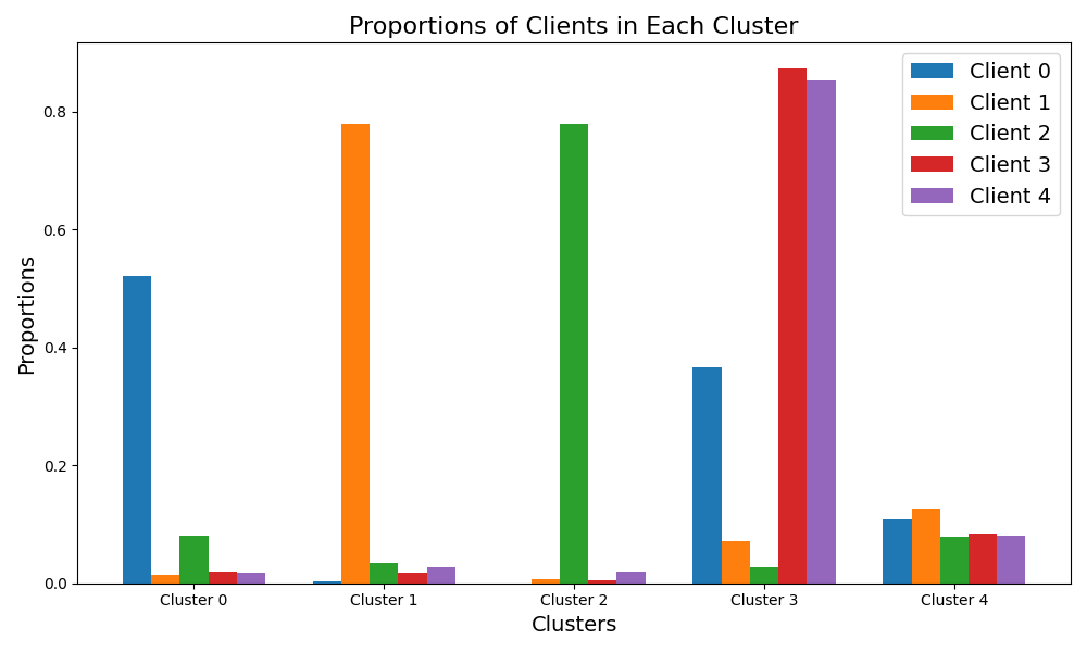
(a) Client Distribution under Local Representation

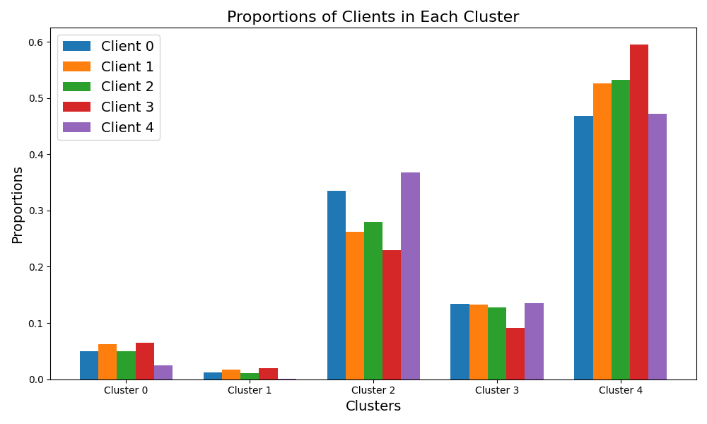
(b) Client Distribution under Global Representation

Figure 2: Comparison Between Local Representation and Global Representation

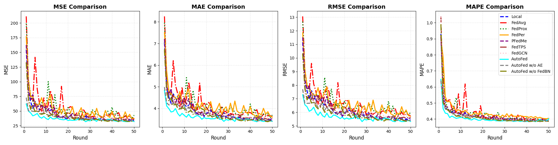
Figure 3: Training Process: This figure shows the change of different metrics in valid set during training.

4.1 Experiment Setup

In our experiments, we compare the performance of our method against several benchmarks, including general FL methods (FedAvg [fedavg], FedProx [fedprox]), PFL methods (FedPer [fedper], pFedMe [pfedme]), and State-Of-The-Art FL methods focused on traffic prediction (FedTPS [zhou2024traffic; zhou2025fedtps], FedGCN [hu2024fedgcn]). To ensure fairness, we employ the same AGCRN architecture as the backbone for all methods. The detailed introduction of these methods is shown in Appendix B. Additionally, we utilize local training (where each client trains a personalized model using their own data) as a baseline. The experiments are conducted on a workstation running Windows 11, equipped with an Intel(R) Core(TM) i7-14700KF processor and an NVIDIA RTX 4080 graphics card.

To validate our method, we conduct two case studies: one for the Travel Demand Prediction (TDP) task and another for the Traffic Flow Prediction (TFP) task, both utilizing real-world datasets. For TDP, we use ride-hailing data from the New York City Taxi and Limousine Commission dataset [deri2015taxi], which includes demand data for Uber and Lyft across five governmental districts in New York City (NYC). Initially, we consider the entire Uber and Lyft data as two separate clients, leading to scenario (i) S0. However, our experiments reveal that this approach is not optimal. In the current configuration, the graph encompasses the entirety of New York City, which is excessively large and may not accurately reflect real-world operational patterns. In practice, traffic demand in Manhattan has limited impact on Queens, as most ride-hailing activities are confined within individual regions. Combining all districts into a single graph can introduce mutual interference, complicating the training process—particularly for models with adaptive adjacency matrices such as AGCRN. We find that dividing the overall graph into several regional subgraphs actually yields better prediction performance (detailed experimental results are presented in the next subsection). Therefore, we propose treating each company within each district as a separate client, although this decision is motivated by modeling effectiveness rather than privacy concerns. We consider three scenarios: (ii) S1: the five Uber clients are trained together; (iii) S2: the five Lyft clients are trained together; (iv) S3: all Uber and Lyft clients are trained together. For TFP, we employ four datasets from the California Transportation Agencies (CalTrans) Performance Measurement System (PEMS) [pems], with each dataset (PEMS03, PEMS04, PEMS07, PEMS08) originating from different regions and time periods on California’s highways. The detailed configuration setup, along with the evaluation metrics, is provided in Appendix C.

4.2 Experiment Results

The experimental results for the TDP and TFP tasks are illustrated in Table 1 and Table 2, respectively. For the TDP task, our AutoFed achieves SOTA performance in almost all scenarios. Notably, we observe two key findings: (i) First, all methods exhibit the worst performance in scenario S0. In comparison to scenarios S1-S3, models in S0 focus on the spatial relationships among districts, resulting in mutual interference due to the limited influence among them. In contrast, scenarios S1-S3 treat the districts as separate clients and leverage FL to aggregate their common temporal relationships, leading to improved performance. (ii) Second, in scenario S3, most methods experience a decline in performance due to the increased diversity of clients compared to S1 and S2. While AutoFed shows improvement on the Uber dataset, there is a slight decrease in performance on the Lyft dataset. Although FedTPS improves on both datasets, it still underperforms relative to AutoFed.

Regarding the TFP task, our method demonstrates performance similar to the two previous SOTA methods for traffic prediction tasks, namely FedTPS and FedGCN. However, it is important to note that both of these methods are highly dependent on hyper-parameters (such as the pattern amount and low-pass filter method in FedTPS, and the number of neighbors in FedGCN), which can lead to significant fluctuations in performance, as reported in their respective papers [zhou2024traffic; zhou2025fedtps; hu2024fedgcn]. In the experiments of these benchmark methods, they model performance is evaluated based on optimal hyper-parameters, which can be challenging to achieve in practice. In contrast, our method does not rely on any hyper-parameter optimization. Moreover, we observe that the performance of FedGCN shows a significant increase in the TFP task compared to the TDP task. This may be due to FedGCN’s design, which considers the potential influence of neighbors within the entire graph. In the TDP task, the neighbors of each client are from different districts, where taxis are seldom transferred among them. Conversely, in the TFP task, all clients are from the same highway, creating a more interconnected relationship.

4.3 Discussions and Analysis

In this section, we further illustrate the efficiency of our method using the scenario S1 in TDP task as an example for principle analysis and an ablation study. First, to analyze the efficacy of each module, we conduct an ablation study, primarily focusing on the FR part. Specifically, we illustrate the model performance when eliminating the AE-denoiser and FedBN in the Adapter, respectively, as shown in Table 1. The results indicate that both modules significantly influence model performance, underscoring the efficacy of our module design. Additionally, we observe that our AutoFed still outperforms other methods in most scenarios, even within the context of the ablation study. This further illustrates the efficiency of our global representation method.

To further explain the efficacy of our proposed method, we analyze the local feature vector $p_{l}$ and the global feature vector $p_{g}$ (i.e., the vectors before and after the adapter in the FR). Specifically, we first combine all $p_{l}$ and $p_{g}$ across clients and then utilize KMeans for clustering. We set the initial cluster centers as the centers of each client. Next, we analyze the proportion of each client within different clusters, as shown in Fig. 2. The results indicate that for the local feature, there are significant differences among clients, leading to the dispersion of local features across different clusters. In contrast, the distribution of global features among clients is relatively uniform within each cluster, suggesting that the global feature $p_{g}$ ignores client-specific characteristics and instead focuses on global common patterns.

Finally, we compare the convergence speed, computational cost, and communication cost during training. Fig. 3 illustrates the change in different metrics as the training rounds increase on the validation set, where AutoFed clearly demonstrates a faster convergence speed compared to the others. Additionally, we present the detailed training costs in Table 3. The results indicate that AutoFed and FedTPS have the lowest communication costs but the highest computation times, as both methods require a prompt generation process.

5 Conclusion

In this paper, we propose a novel personalized federated traffic prediction framework named AutoFed. Our method comprises a personalized predictor trained locally to adapt to local data distributions and a federated representor that transforms non-IID input data among clients into a common global representation, serving as a guiding prompt for the personalized predictor’s decoding process. Compared to conventional methods, our approach eliminates the need for manual feature design or hyper-parameter tuning, making it more practical, as these settings often depend on prior knowledge of clients or datasets. Through validation on real-world travel demand prediction and traffic flow prediction datasets, our method demonstrates superior performance with reduced communication costs. In the future, it would be worthwhile to explore the applicability of our method in more general time series prediction scenarios.

Impact Statement

We believe this work raises minimal ethical concerns, as Federated Learning is designed to prioritize privacy protection.

Appendix A Algorithm

The detailed process of our AutoFed is illustrated in Algorithm 1.

Algorithm 1 Training Process of AutoFed

0: Number of clients $n$, local datasets $\{D_{i}\}_{i=1}^{n}$, shared model parameters $\Theta^{0}$, personal model parameters $\{\theta_{i}^{0}\}_{i=1}^{n}$, communication rounds $M$, local epochs $E$

0: Personalized models $\{\theta_{i}^{M},\Theta^{M}\}_{i=1}^{n}$

1: Server executes:

2: Initialize shared parameters $\Theta^{0}$

3: Broadcast $\Theta^{0}$ to all clients

4: for each communication round $m=0,1,\dots,M-1$ do

5:  Randomly select a subset of clients $S_{m}\subseteq\{1,\dots,n\}$

6:  for each client $i\in S_{m}$ in parallel do

7:   $\theta_{i}^{m+1},\Delta\Theta_{i}^{m}\leftarrow\text{ClientUpdate}(i,\theta_{i}^{m},\Theta^{m})$

8:  end for

9:  Aggregate shared parameters: $\Theta^{m+1}\leftarrow\Theta^{m}+\frac{1}{|S_{m}|}\sum_{i\in S_{m}}\Delta\Theta_{i}^{m}$

10:  Broadcast $\Theta^{m+1}$ to all clients

11: end for

12: 

13: ClientUpdate(client $i$, personal parameters $\theta_{i}$, shared parameters $\Theta$):

14: Initialize local shared parameters: $\Theta_{i}\leftarrow\Theta$

15: for each local epoch $e=1$ to $E$ do

16:  for each batch $(X_{b},Y_{b})\in D_{i}$ do

17:   Forward Pass:

18:   Compute denoised features: $\hat{X}_{b}=\text{AE-dec}(\text{AE-enc}(X_{b}))$

19:   Extract local features: $p_{l}=\text{Encoder}(X_{b})$

20:   Generate global prompt: $p_{g}=\text{Adapter}(p_{l})$

21:   Generate predictions: $\hat{Y}_{b}=\text{PP}(X_{b},p_{g})$

22:   Loss Computation:

23:   Compute AE loss: $L^{ae}=\text{MAE}(X_{b},\hat{X}_{b})$

24:   Compute prediction loss: $L^{pre}=\text{MAE}(Y_{b},\hat{Y}_{b})$

25:   Compute adaptive weight: $\alpha=\frac{L^{ae}}{L^{pre}}$

26:   Compute total loss: $L=L^{pre}+\alpha\cdot L^{ae}$

27:   Backward Pass:

28:   Update $\theta_{i}$ and $\Theta_{i}$ via gradient descent: $\nabla_{\theta_{i},\Theta_{i}}L$

29:  end for

30: end for

31: Compute parameter update: $\Delta\Theta_{i}=\Theta_{i}-\Theta$

32: Return $\theta_{i}$, $\Delta\Theta_{i}$

Appendix B Introduction of Comparative Methods

• FedAvg [fedavg]: This classical FL method enables each client to train on their individual data at each round, after which the server parameters are updated to the average of all clients’ parameters, which are then distributed before the next round.

• FedProx [fedprox]: FedProx introduces a proximal term to the loss function of FedAvg, preventing the local model from deviating too far from the global model. However, it still aims to optimize a global model rather than personalized ones.

• FedPer [fedper]: As a classical PFL method, FedPer allows different clients to share a common base layer for robust feature extraction while maintaining personalized output layers for tailored results.

• pFedMe [pfedme]: pFedMe is a PFL framework that utilizes Moreau envelopes as a regularized loss function, enabling each client to efficiently find its optimal model while leveraging global information.

• FedTPS [zhou2024traffic; zhou2025fedtps]: Similar to our method, FedTPS employs a low-pass filter for stable pattern extraction and a pattern repository for prompt generation. However, these processes require manual settings and hyper-parameter tuning, and the aggregation in the pattern repository is based on similarity among clients, leading to higher computational costs.

• FedGCN [hu2024fedgcn]: FedGCN is based on the assumption that potential neighbor nodes of all real nodes exist within the graph. It introduces the MendGCN module to consider these external factors.

Appendix C Experiment Details

In all experiments, we set the ratio of training, validation, and testing sets to 6:2:2. For the TDP task, we reproduce all comparative methods ourselves, setting the batch size to 128, the communication rounds to 50 with a local epoch of 1, and the learning rate to $10^{-3}$ using the Adam optimizer.

The results for the TFP task are sourced from [zhou2024traffic; zhou2025fedtps; hu2024fedgcn]. To ensure fairness in the TFP task, we follow the same settings as [zhou2024traffic; zhou2025fedtps], adjusting the communication rounds to 200 and setting the client amount to 4. Additionally, we employ the same techniques such as column learning, gradient clipping, and the MultiStepLR scheduler provided in their official repository.

During experiment, we consider the following evaluation metrics: Mean Absolute Error (MAE), Root Mean Square Error (RMSE), Mean Square Error (MSE), and Mean Absolute Percentage Error (MAPE):

MAE $$=\|\hat{y}-y\|_{1}\ ,$$ (7)

RMSE $$=\sqrt{\|\hat{y}-y\|_{2}^{2}}\ ,$$

MSE $$=\|\hat{y}-y\|_{2}^{2}\ ,$$

MAPE $$=\left\|\frac{\hat{y}-y}{y}\right\|_{1}\ ,$$

where $\|\cdot\|_{2}$ denotes the $L_{2}$ norm.