Dynamic Phase Transitions in Periodically Driving 1D Ising Model

Abstract

This work investigates dynamical quantum phase transitions (DQPTs) in a one-dimensional Ising model subjected to a periodically modulated transverse field. In contrast to sudden quenches, we demonstrate that DQPTs can be induced in two distinct ways. First, when the system remains within a given phase–ferromagnetic (FM) or paramagnetic (PM), a resonant periodic drive can trigger a DQPT when its frequency matches the energy-level transition of the system. The timescale for the transition is governed by the perturbation strength $\lambda^{\prime}$, the critical mode $k_{c}$, and its energy gap $\Delta_{k_{c}}$, following the scaling relation $\tau\propto\sin^{-1}k_{c}\Delta_{k_{c}}\lambda^{\prime-1}$. Second, for drives across the critical point between the FM and PM phases, low frequencies can always induce DQPTs, regardless of resonance. This behavior stems from the degeneracy of the energy-level at the critical point, which ensures that any drive with a frequency lower than the system’s intrinsic transition frequency will inevitably excite the system. However, in the high-frequency regime, such excitation will be strongly suppressed, thereby inhibiting the occurrence of DQPTs. This study provides deeper insight into the nonequilibrium dynamics of quantum spin chains.

I Introduction

With these experimental advances for exploring the non-equilibrium dynamics of confined quantum systems such as ultracold atoms [doi:10.1126/science.aaa7432, Jotzu2014, PhysRevLett.109.020505], Rydberg atoms [RevModPhys.82.2313], superconducting qubits [PhysRevB.111.224301], and ion traps [PhysRevA.81.022306, PhysRevA.105.022616], an in-depth study of the dynamics of quantum many-body systems far from thermodynamic equilibrium becomes possible. Dynamical quantum phase transitions (DQPTs) have recently emerged as an interesting phenomenon within this regime [Heyl2013, PhysRevB.93.085416, RevModPhys.83.863, PhysRevLett.95.105701, Heyl_2018, Heyl_2019, Heyl2013, PhysRevLett.115.140602], which serve as a nonequilibrium counterpart to equilibrium phase transitions. The concept of DQPT arises from the analogy between the equilibrium partition function of a system and the Loschmidt amplitude, which measures the overlap between an initial state and its time-evolved state [PhysRevLett.115.140602, PhysRevLett.96.140604, PhysRevB.99.054302, PhysRevLett.118.015701, PhysRevE.88.052122, PhysRevB.102.104305, Najafi_2019, PhysRevLett.124.160603, PhysRevB.97.205103, Mukherjee_2019]. As equilibrium phase transitions are signaled by nonanalyticities in thermal free energy, DQPTs are revealed through nonanalytical behavior in dynamical free energy [PhysRevB.89.125120, PhysRevB.87.195104, PhysRevB.89.161105, PhysRevA.103.012204, PhysRevB.91.155127, Mendoza-Arenas_2022, PhysRevB.106.054308, PhysRevLett.124.160603, PhysRevLett.126.040602, PhysRevB.97.064304, PhysRevB.97.045147, PhysRevB.107.085116, Khan2023], with real time serving as the control parameter [Heyl_2019, PhysRevB.87.195104, PhysRevB.90.125106, PhysRevLett.113.265702, PhysRevLett.96.136801, PhysRevB.101.245148, PhysRevLett.126.040602, PhysRevB.104.085104, PhysRevB.103.144305, PhysRevB.97.235144]. The non-analyticity in quantum state evolution is accompanied by universal critical exponents, unveiling scaling behavior and universality class patterns near quantum critical times [PhysRevB.97.134306, PhysRevLett.115.140602, 9zwv-s4bn, PhysRevB.104.115159]. Furthermore, analogous to order parameters in equilibrium quantum phase transitions, a dynamical topological order parameter has been proposed to capture DQPTs [PhysRevB.97.134306, Sharma_2014, PhysRevB.96.180303, PhysRevLett.103.056403]. Experimentally, DQPT has been realized on various quantum simulators, such as ultracold atoms [Fläschner2018], trapped ions [PhysRevLett.119.080501], superconducting quantum circuits [PhysRevApplied.11.044080], etc [10.1063/5.0004152, PhysRevLett.122.020501, Xu2020, Zhang2025].

DQPT was originally proposed in the context of quench dynamics within a nearest‑neighbor transverse‑field Ising model [Heyl2013, PhysRevLett.115.140602, PhysRevB.97.134306, PhysRevB.107.L121113], where the transverse field of the system Hamiltonian is suddenly changed. It was later extended to finite‑time slow quench processes [PhysRevB.81.012303, PhysRevA.98.063601, PhysRevB.106.224302, PhysRevA.110.042209, PhysRevA.84.013615, PhysRevA.102.042222]. Due to the critical slowing‑down effect near a quantum phase transition, crossing the critical point at any finite rate inevitably excites the system, thereby making quantum coherence an essential feature of such transitions—a behavior captured by the Kibble–Zurek mechanism [PhysRevB.81.012303, PhysRevA.98.063601, PhysRevB.106.224302, PhysRevA.101.023610, PhysRevB.92.035117, PhysRevLett.131.230401]. Notably, quantum coherence not only restores DQPTs that would otherwise be destroyed by thermal fluctuations, but can also give rise to entirely new DQPTs that are independent of the equilibrium quantum critical point [Xu_2024]. In recent years, periodically driven systems have opened a new avenue for exploring DQPTs [PhysRevE.96.052105, mkll-nd46, PhysRevB.82.235114, PhysRevLett.126.020602, PhysRevResearch.3.013097, PhysRevB.90.125106, Bordia2017, PhysRevA.111.022430, PhysRevB.98.245144]. Unlike conventional quench dynamics, periodic driving allows Hamiltonian parameters to be modulated in diverse ways [PhysRevE.96.052105], leading to a wide range of experimental schemes and platforms for realizing driven settings. Although numerous studies have examined DQPTs from various perspectives, a comprehensive understanding of their underlying mechanisms remains elusive.

To address this issue, this work studies DQPTs in a one-dimensional Ising model driven by a periodic transverse field. Using time-dependent perturbation theory, we examine the roles of the driving intensity and frequency, which elucidates the underlying mechanism of DQPTs. Our results show that the driving frequency is crucial for the occurrence of a DQPT. Specifically, a DQPT arises when the driving frequency resonates with the energy-level transition frequency of the system. The driving strength, together with the critical mode and its energy gap, governs the timescale required for the DQPT to occur, satisfying the scaling law $\tau\propto\sin^{-1}k_{c}\Delta_{k_{c}}\lambda^{\prime-1}$. Furthermore, we show that low‑frequency perturbations that cross the equilibrium critical point can also induce DQPTs, whereas high‑frequency drives strongly suppress the evolution of the system.

The structure of this paper is as follows: Sec. II introduces the Periodic driving Ising model and reviews the basic concepts of DQPT. In Sec. III, we elucidate the roles of the frequency and the strength of the drive on DQPT when the system remains within the same equilibrium phase. Sec. IV investigates the influences of periodic driving on DQPTs when the system crosses the equilibrium quantum critical point. Finally, Sec. V closes the paper with some concluding remarks.

II Model and Periodic Driving Protocol

The Hamiltonian of the one-dimensional transverse field Ising model is

$$\hat{H}=-\frac{J}{2}\sum_{j=1}^{N}\bigl[\hat{\sigma}_{j}^{z}\hat{\sigma}_{j+1}^{z}+\lambda\hat{\sigma}_{j}^{x}\bigr],$$ (1)

where $\hat{\sigma}^{\alpha}_{j}$ $(\alpha=x,y,z)$ is the spin-1/2 Pauli operator at lattice site $j$ and the periodic boundary condition is imposed as $\hat{\sigma}^{\alpha}_{N+1}=\hat{\sigma}^{\alpha}_{1}$. Here we only consider that $N$ is even. $J$ is longitudinal spin-spin coupling, and we set $J=1$ as the overall energy scale without loss of generality. $\lambda$ is a dimensionless parameter measuring the strength of the transverse field with respect to the longitudinal spin-spin coupling. Driven by the transverse field $\lambda$, a quantum phase transition from the FM phase ($\lambda<1$) to the PM phase ($\lambda>1$), which is known as the Ising transition, occurs at the critical point of $\lambda_{c}=1$.

This Hamiltonian is integrable and can be mapped to a system of free fermions and therefore be solved exactly. By applying the Jordan-Wigner transformation and the Fourier transformation, the Hamiltonian converts from spin operators into spinless fermionic operators as [10.21468/SciPostPhys.1.1.003]

$$\hat{H}=\sum_{k>0}\begin{pmatrix}\hat{c}^{\dagger}_{k}&\hat{c}_{-k}\end{pmatrix}\begin{pmatrix}\lambda-\cos k&-i\sin k\\ i\sin k&-\lambda+\cos k\end{pmatrix}\begin{pmatrix}\hat{c}_{k}\\ \hat{c}^{\dagger}_{-k}\end{pmatrix},$$ (2)

where $\hat{c}_{k}$ and $\hat{c}^{\dagger}_{k}$ are respectively fermion annihilation and creation operators for mode $k=(2n-1)\pi/N$ with $n=1,2,\cdots,N/2$, corresponding to antiperiodic boundary conditions when $N$ is even. The energy levels of $\hat{H}_{k}$ are

$$\varepsilon^{\pm}_{k}=\pm\varepsilon_{k}=\pm\sqrt{(\lambda-\cos k)^{2}+\sin^{2}k},$$ (3)

with the corresponding eigenvectors

$$\begin{split}|\varepsilon^{+}_{k}\rangle&=\biggl[i\sin\frac{\theta_{k}}{2}+\cos\frac{\theta_{k}}{2}\hat{c}^{\dagger}_{k}\hat{c}^{\dagger}_{-k}\biggr]|0\rangle,\\ |\varepsilon^{-}_{k}\rangle&=\biggl[\cos\frac{\theta_{k}}{2}+i\sin\frac{\theta_{k}}{2}\hat{c}^{\dagger}_{k}\hat{c}^{\dagger}_{-k}\biggr]|0\rangle,\end{split}$$ (4)

where $|0\rangle$ is the vacuum state. The angle $\theta_{k}$, which is generally complex, is determined by $\tan\theta_{k}=\sin k/(\lambda-\cos k)$.

At time $t<0$, the system is prepared in the ground state

$$|G\rangle=\bigotimes_{k>0}|\varepsilon^{-}_{k}\rangle.$$ (5)

A periodic perturbation is then switched on at $t=0$, characterized by the transverse field

$$\lambda(t)=\lambda+\lambda^{\prime}\cos(\omega t),$$ (6)

with amplitude $\lambda^{\prime}$ and frequency $\omega$. The dynamics of the system is governed by the perturbed Hamiltonian $\hat{H}(t)$, and the system state at time $t$ is determined by ($\hbar=1$)

$$|\psi(t)\rangle=\mathcal{T}\exp\Bigl[-i\int_{0}^{t}\hat{H}(t^{\prime})dt^{\prime}\Bigr]|G\rangle,$$ (7)

where $\mathcal{T}$ denotes the time-ordering operator. The instantaneous state can be expressed in a tensor product form as $|\psi(t)\rangle=\bigotimes_{k>0}|\psi_{k}(t)\rangle$, where each mode evolves as

$$|\psi_{k}(t)\rangle=(v_{k}(t)+u_{k}(t)c_{k}^{\dagger}c_{-k}^{\dagger})|0\rangle.$$ (8)

The coefficients $u_{k}(t)$ and $v_{k}(t)$ can be obtained by solving the differential equation

$$\frac{d}{dt}\begin{pmatrix}u_{k}(t)\\ v_{k}(t)\end{pmatrix}=-i\begin{pmatrix}\lambda(t)-\cos k&-i\sin k\\ i\sin k&-\lambda(t)+\cos k\end{pmatrix}\begin{pmatrix}u_{k}(t)\\ v_{k}(t)\end{pmatrix}.$$ (9)

The main goal of this paper is to investigate DQPT induced by periodic driving. The theory of DQPT is built upon the Loschmidt overlap amplitude,

$$\mathcal{G}(t)=\langle G|\psi(t)\rangle=\prod_{k>0}\langle\varepsilon^{-}_{k}|\psi_{k}(t)\rangle,$$ (10)

which measures the overlap between the time-evolved and initial states. A DQPT is signaled by the vanishing of this amplitude, indicating orthogonality between $|\psi(t)\rangle$ and $|G\rangle$. This criticality is identified by a non-analytic cusp in the dynamical free energy density, or the rate function,

$$r(t)=-\frac{1}{\pi}\int_{0}^{\pi}dk\ln|\langle\varepsilon^{-}_{k}|\psi_{k}(t)\rangle|^{2},$$ (11)

serving as the counterpart of the free energy in equilibrium phase transitions. Moreover, DQPTs are endowed with topological properties, characterized by a dynamical topological invariant defined as [PhysRevB.96.014302]

$$\nu(t)=\frac{1}{2\pi}\int_{0}^{\pi}\frac{\partial\phi_{k}^{G}(t)}{\partial k}dk,$$ (12)

which undergoes a quantized jump at the critical times of the DQPT. The underlying geometric phase is defined as

$$\phi_{k}^{G}(t)=\phi_{k}(t)-\phi_{k}^{D}(t),$$ (13)

where

$$\phi_{k}(t)=\arg\mathcal{G}_{k}(t)$$ (14)

is the total phase, and

$$\phi_{k}^{D}(t)=-\int_{0}^{t}\langle\psi_{k}(t^{\prime})|\hat{H}_{k}(t^{\prime})|\psi_{k}(t^{\prime})\rangle dt^{\prime}.$$ (15)

is the dynamical phase.

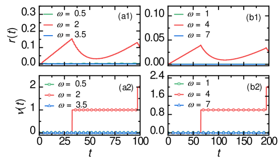
Figure 1: (Color online) Time evolution of the rate function $r(t)$ and the winding number $\nu(t)$ under different driving frequencies. Panel (a1-a2) depicts the magnetic field initially fixed within the FM phase $\lambda=0.5$, with a resonance frequency range of $[1,3]$. Panel (b1-b2) depicts the magnetic field initially fixed within the PM phase $\lambda=2$, with a resonance frequency range of $[2,6]$. The driving strength is $\lambda^{\prime}=0.1$ for all the cases.

III The Influence of periodic driving Within the Same phase

In this section, we explore the emergence of DQPTs driven by periodic driving within the FM phase ($\lambda<1,~\lambda+\lambda^{\prime}<1$) or PM phase ($\lambda>1,~\lambda-\lambda^{\prime}>1$). First, we investigate the effects of the frequency of periodic driving. Fig. 1 illustrates the time evolution of the Loschmidt echo rate function and the winding number for different frequencies. The results demonstrate a critical dependence of DQPTs on the driving frequency. Pronounced non-analytic signatures are observed only when the driving frequency $\omega$ is tuned to a specific regime, for instance, $\omega=2$ for $\lambda=0.5$ (FM phase) or $\omega=4$ for $\lambda=2$ (PM phase). Under these resonant conditions, the rate function exhibits clear oscillatory behavior with periodic cusp singularities. Concurrently, the winding number, which remains quantized during the dynamics, undergoes discrete integer jumps precisely at the critical times where the cusps appear. The simultaneous occurrence of these features provides definitive evidence for a DQPT. By contrast, when the driving frequency is detuned from these specific values, the rate function stays close to zero throughout the evolution, indicating that the system does not evolve significantly from its initial state, and no DQPT occurs. These observations underscore that the resonant frequency plays a crucial role in the occurrence of DQPT.

A comparison between the results of periodic driving and sudden quench dynamics is essential. Although a sudden quench performed within a given phase of the Ising model cannot induce a DQPT [Cao_2022, 10.21468/SciPostPhys.1.1.003], we demonstrate here that a periodic perturbation applied within the same phase can indeed trigger a DQPT, provided that the driving frequency is tuned into an appropriate range. This crucial frequency dependence originates from transitions among the system’s energy levels, revealing the physical mechanism behind DQPT.

As clarified by time-dependent perturbation theory (see Appendix for details), a periodic perturbation can efficiently drive transitions between energy levels only when its frequency resonates with the intrinsic energy gap of the system. Such resonant driving is necessary for the system to evolve far from its initial state and undergo a DQPT. In contrast, off-resonant perturbations have negligible effects, leaving the system essentially unchanged. From the energy dispersion $\varepsilon_{k}=\sqrt{\lambda^{2}-2\lambda\cos k+1}$, the energy gap $\Delta_{k}=2\varepsilon_{k}$ varies over the interval $2|\lambda-1|\leq\Delta_{k}\leq 2|\lambda+1|$ as $k$ goes from $0$ to $\pi$. Therefore, whenever the perturbation frequency lies within this interval, there always exists a critical mode $k_{c}=\arccos\bigl(\frac{\lambda^{2}+1-\omega^{2}/4}{2\lambda}\bigr)$ that triggers the DQPT. It should be noted that perturbations with the boundary frequencies $2|\lambda-1|$ and $2|\lambda+1|$ do not induce a DQPT, because the corresponding critical modes are $\pi$ and $0$, respectively. In these cases, the Hamiltonians before and after the perturbation commute, so the initial ground state remains unchanged and does not evolve, let alone undergo a DQPT.

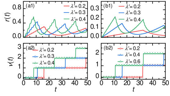
Figure 2: (Color online) Time evolution of the rate function $r(t)$ and the winding number $\nu(t)$ under different disturbance intensities. Panel (a1-a2) depicts the evolutionary process within the FM phase (where $\lambda=0.5$, $\omega=2$), with a resonance frequency range of $[1,3]$. Panel (b1-b2) depicts the evolutionary process within the PM phase (where $\lambda=2$, $\omega=4$), with a resonance frequency range of $[2,6]$.

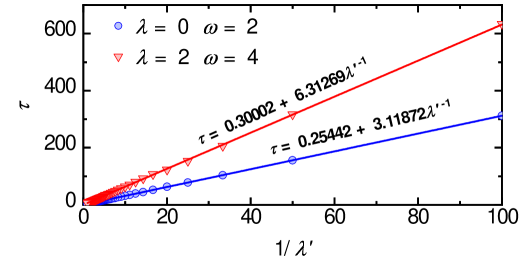
Figure 3: (Color online) The scaling of the evolution time and the driving strength with $\lambda=0$, $\omega=2$ and $\lambda=2$, $\omega=4$.

Next, we examine how the strength of the perturbation influences DQPT. Fig. 2 shows the effect of varying the perturbation strength on the first critical time at which DQPT occurs for a fixed resonant frequency. It is observed that as the strength $\lambda^{\prime}$ increases, the first critical time becomes shorter. This trend holds consistently in both the FM and PM phases. We interpret this first critical time as the characteristic time $\tau$ required to induce the DQPT.

To establish a quantitative relationship between the perturbation strength $\lambda^{\prime}$ and the DQPT onset time $\tau$, we analyze their scaling behavior. Fig. 3 shows the dependence of $\tau$ on the perturbation strength $\lambda^{\prime}$ at a fixed resonant frequency, with the system initialized in the FM phase ($\lambda=0$, $\omega=2$) and the PM phase ($\lambda=2$, $\omega=4$). In both cases, the time required to induce a DQPT scales inversely with the perturbation strength, following $\tau\sim c\lambda^{\prime-1}$. This inverse scaling can be understood within perturbation theory (see Appendix for details). The amplitude of the excited state evolves as $a_{k}^{+}(t)\approx\lambda^{\prime}\sin\theta_{k}t$, implying that the characteristic time for exciting the system scales as $t\propto(\lambda^{\prime}|\sin\theta_{k}|)^{-1}$. This excitation causes the return probability to the ground state to vanish, thereby inducing a DQPT. Since the DQPT is governed by the critical mode $k_{c}$, the onset time $\tau$ corresponds precisely to the energy-level-transition time at $k_{c}$: $\tau\propto(\lambda^{\prime}|\sin\theta_{k_{c}}|)^{-1}$. Using the relation $\sin\theta_{k}=\sin k/\epsilon_{k}=2\sin k/\Delta_{k}$, we derive the scaling law for the DQPT onset time:

$$\tau\propto\sin^{-1}k_{c}\Delta_{k_{c}}\lambda^{\prime-1},$$ (16)

where $\Delta_{k_{c}}$ denotes the energy gap corresponding to the critical mode $k_{c}$. This relationship indicates that a larger energy gap results in a longer DQPT onset time $\tau$, since it directly extends the duration needed for the system to undergo the underlying energy-level transition. Remarkably, an arbitrarily weak perturbation is sufficient to induce a DQPT, provided the evolution time is sufficiently long. However, if the critical mode is $k_{c}=0$ or $\pi$, the onset time $\tau$ diverges, and consequently no DQPT occurs–consistent with our earlier conclusion. Conversely, the onset time is minimized when the critical mode is $k_{c}=\pi/2$.

For the representative FM case $(\lambda=0,\omega=2)$, all modes except $k=0$ and $k=\pi$ become critical that are capable of inducing DQPTs. Among these, the critical mode $k_{c}=\pi/2$ yields the shortest onset time: $\tau_{1}\propto 2\lambda^{\prime-1}$. In contrast, for the PM phase $(\lambda=2,\omega=4)$, the critical mode is $k_{c}=\arccos(1/4)$, leading to an onset time: $\tau_{2}\propto 16/(\sqrt{15}\,\lambda^{\prime})$. Consequently, the time required to trigger a DQPT in the PM phase is approximately twice that in the FM phase, as illustrated in Fig. 3. This observation provides clear confirmation of the scaling law presented in Eq. (16).

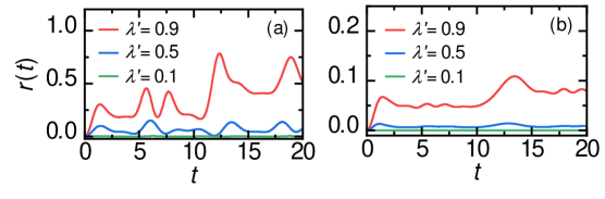
Figure 4: (Color online) The time evolution of the rate function in the (a) FM ($\lambda=0$) and (b) PM ($\lambda=2$) phases for different driving intensities. The frequency is $\omega=0.5$ for all cases.

A natural question is whether increasing the intensity of the detuning perturbation can induce a DQPT. To address this, we calculate the rate function for different perturbation intensities, as shown in Fig. 4. It can be seen that the rate function increases with the perturbation strength in both the FM and PM phases, but the cusp singularity cannot be observed, indicating that DQPTs cannot be induced solely by enhancing the detuning perturbation.

IV The Influence of periodic driving across the critical point

In this section, we examine perturbations that drive the system across the critical point at $\lambda_{c}=1$, specifically in the regime where $\lambda<1$ and $\lambda+\lambda^{\prime}>1$. Since Fig. 1 established that any driving with frequency within the resonance interval $2|\lambda-1|<\omega<2|\lambda+1|$ invariably induces a DQPT, we focus here on off-resonant frequencies outside this range. Fig. 5 shows the time evolution of the Loschmidt echo rate function and the winding number for the protocol $\lambda(t)=0.5+2\cos(\omega t)$, with $\omega=0.5$ (low frequency) and $\omega=6$ (high frequency). The results demonstrate that low-frequency interphase perturbations can indeed induce DQPTs, as signaled by the characteristic cusp singularities in the rate function and discrete jumps in the winding number. In contrast, under the influence of high-frequency interphase perturbations, the system does not evolve significantly, let alone DQPT.

It is well known that an interphase quench, which corresponds to the limiting case of $\omega=0$ in our setup, guarantees a DQPT [PhysRevA.110.042209, PhysRevB.96.180303, 10.21468/SciPostPhys.1.1.003]. In this light, our findings indicate that, while low-frequency perturbations maintain this behavior, high-frequency driving can effectively suppress the occurrence of DQPTs. This distinction can be understood from the following physical picture. Under low-frequency driving, the system has sufficient time to respond to the slow change of the Hamiltonian, facilitating its evolution. Although the driving frequency is off-resonant with the system’s intrinsic transition frequencies, the system can still be driven into the excited states, because the driving is across the critical point. This is because, at the critical point $\lambda_{c}=1$, the ground-state energy level becomes degenerate and the energy gap closes. The vanishing gap between the ground state and the first excited state renders it exceedingly difficult for the system to pass through the critical region without generating excitations, thereby triggering a DQPT. Conversely, under high-frequency driving, the extremely short period of the external perturbation hinders the system’s ability to respond, effectively suppressing its evolution and preventing a DQPT.

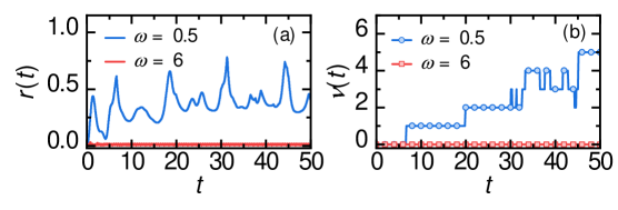
Figure 5: (Color online) The time evolution of the rate function (a) and the winding number (b) at different drive frequencies when the transverse magnetic field crosses the quantum critical point, where $\lambda=0.5$ and $\lambda^{\prime}=2$.

V Conclusions

This work investigated dynamical quantum phase transitions (DQPTs) induced by periodic driving in a one-dimensional Ising model, focusing on the rate function and the winding number. We found that unlike sudden quenchs, periodic perturbation applied within the same phase can induce a DQPT, as long as the driving frequency resonates with the frequency of the transition between the energy levels of the system. This resonant effect stems from driving‑induced transitions between the system’s energy levels. The timescale for the occurrence of a DQPT is governed by the perturbation strength, the critical mode, and its energy gap, following the scaling relation $\tau\propto\sin^{-1}k_{c}\Delta_{k_{c}}\lambda^{\prime-1}$. Furthermore, we examined perturbations that cross the equilibrium critical point, demonstrating that low‑frequency drives can trigger DQPTs, whereas high‑frequency drives strongly suppress the system’s evolution. Compared with conventional quench protocols, periodic perturbations offer a more refined means to control DQPTs, thereby providing a new perspective for the study of non‑equilibrium dynamics in quantum many‑body systems.

Appendix A Time-dependent perturbation theory

Under a transverse field perturbation, the Hamiltonian for mode $k$ can be decomposed into two parts:

$$\hat{H}_{k}(t)=\hat{H}_{k}+\hat{H}^{\prime}_{k}(t),$$ (17)

where,

$$\hat{H}_{k}=\begin{pmatrix}\lambda-\cos k&-i\sin k\\ i\sin k&-\lambda+\cos k\end{pmatrix}$$ (18)

denotes the unperturbed Hamiltonian, and

$$\hat{H}^{\prime}_{k}(t)=\begin{pmatrix}\lambda^{\prime}\cos\omega t&0\\ 0&-\lambda^{\prime}\cos\omega t\end{pmatrix},$$ (19)

represents the time dependent perturbation. The time-evolved state under this perturbation can be represented as

$$|\psi_{k}(t)\rangle=a_{k}^{+}(t)e^{-i\varepsilon_{k}t}|\varepsilon^{+}_{k}\rangle+a_{k}^{-}(t)e^{i\varepsilon_{k}t}|\varepsilon^{-}_{k}\rangle.$$ (20)

The coefficient $a^{\pm}_{k}(t)$ admit a perturbative expansion:

$$a^{\pm}_{k}(t)=a_{k}^{\pm(0)}(t)+a_{k}^{\pm(1)}(t)+\cdots,$$ (21)

where $a_{k}^{\pm(0)}(t)$ and $a_{k}^{\pm(1)}(t)$ denote the zeroth- and the first-order perturbation corrections respectively. In this paper, only these two terms are considered. The evolution of the perturbation coefficients satisfies the following equations

$$\dot{a}_{k}^{\pm(0)}(t)=0,$$ (22)

and

$$\dot{a}_{k}^{\pm(1)}(t)=-ia_{k}^{\pm(0)}\hat{H^{\prime}}_{k}^{\pm,\pm}(t)-ia_{k}^{\mp(0)}e^{\pm i2\varepsilon_{k}t}\hat{H^{\prime}}_{k}^{\pm,\mp}(t),$$ (23)

where $\hat{H^{\prime}}_{k}^{\pm,\pm}(t)=\langle\varepsilon_{k}^{\pm}|\hat{H}^{\prime}_{k}(t)|\varepsilon_{k}^{\pm}\rangle=\pm\cos\theta_{k}\lambda^{\prime}\cos\omega t$ and $\hat{H^{\prime}}_{k}^{\pm,\mp}(t)=\langle\varepsilon_{k}^{\pm}|\hat{H}^{\prime}_{k}(t)|\varepsilon_{k}^{\mp}\rangle=\pm i\sin\theta_{k}\lambda^{\prime}\cos\omega t$. For the initial ground state $|\varepsilon_{k}^{-}\rangle$, the zeroth-order coefficients are

$$a^{+(0)}_{k}=0,~~a^{-(0)}_{k}=1,$$ (24)

and first-order approximation coefficients are given by

$$\begin{split}a_{k}^{+(1)}&=\lambda^{\prime}\sin\theta_{k}\biggl[\frac{e^{i(2\varepsilon_{k}-\omega)t}-1}{i(2\varepsilon_{k}-\omega)}+\frac{e^{i(2\varepsilon_{k}+\omega)t}-1}{i(2\varepsilon_{k}+\omega)}\biggr],\\ a_{k}^{-(1)}&=i\lambda^{\prime}\cos\theta_{k}\frac{\sin\omega t}{\omega}.\end{split}$$ (25)

When the driving frequency resonates with the system transition frequency, i.e., $\omega=2\varepsilon_{k}$, the first-order coefficients simplify to

$$\begin{split}a_{k}^{+(1)}&\approx\lambda^{\prime}\sin\theta_{k}t,\\ a_{k}^{-(1)}&\approx 0,\end{split}$$ (26)

where the high-frequency oscillation terms have been neglected. This shows that under resonant driving, the probability amplitude of the excited state grows linearly in time, indicating that the system undergoes a transition into the excited state. The timescale for this transition is inversely proportional to the perturbation strength

$$t_{k}\propto\lambda^{\prime-1}\sin^{-1}\theta_{k}.$$ (27)

According to the definition of $\sin\theta_{k}=\frac{\sin k}{\varepsilon_{k}}=\frac{2\sin k}{\Delta_{k}}$, this transition timescale is jointly determined by energy gap and perturbation strength:

$$t_{k}\propto\sin^{-1}k\Delta_{k}\lambda^{\prime-1}.$$ (28)