MultiRisk: Multiple Risk Control via Iterative Score Thresholding
Abstract
As generative AI systems are increasingly deployed in real-world applications, regulating multiple dimensions of model behavior has become essential. We focus on test-time filtering: a lightweight mechanism for behavior control that compares performance scores to estimated thresholds, and modifies outputs when these bounds are violated. We formalize the problem of enforcing multiple risk constraints with user-defined priorities, and introduce two efficient dynamic programming algorithms that leverage this sequential structure. The first, MULTIRISK-BASE, provides a direct finite-sample procedure for selecting thresholds, while the second, MULTIRISK, leverages data exchangeability to guarantee simultaneous control of the risks. Under mild assumptions, we show that MULTIRISK achieves nearly tight control of all constraint risks. The analysis requires an intricate iterative argument, upper bounding the risks by introducing several forms of intermediate symmetrized risk functions, and carefully lower bounding the risks by recursively counting jumps in symmetrized risk functions between appropriate risk levels. We evaluate our framework on a three-constraint Large Language Model alignment task using the PKU-SafeRLHF dataset, where the goal is to maximize helpfulness subject to multiple safety constraints, and where scores are generated by a Large Language Model judge and a perplexity filter. Our experimental results show that our algorithm can control each individual risk at close to the target level.
1 Introduction
As generative AI models are increasingly deployed in real-world applications, from healthcare (mesko2023imperative) to education (su2023unlocking), ensuring the quality and reliability of their outputs has become a central concern. Users and developers alike must be able to regulate model behavior to meet standards of safety, fairness, creativity, and helpfulness.
Quality control can be implemented at multiple stages of the generative pipeline. During pre-training, data curation techniques such as filtering, deduplication, and tagging have been shown to improve the quality and safety of outputs (lee2022deduplicating; penedo2023refinedweb; maini2025safety). During post-training, alignment techniques such as Reinforcement Learning from Human Feedback (RLHF) (ouyang2022training) and its variants (bai2022training; bai2022constitutional; dai2024safe) steer model behavior towards human preferences expressed over pairs of completions.
In contrast, test-time filtering offers a lightweight mechanism for regulating model behavior without retraining or modifying weights. These methods apply post-hoc changes to model outputs by computing a relevant score, comparing it to a learned threshold, and modifying responses that exceed tolerance levels. For example, if an unsafety score for generated text is too high, the system may choose not to output the completion.
In practice, model providers seek to regulate several performance metrics simultaneously, such as safety, reliability, creativity, and helpfulness. Recent work highlights a growing need for multi-criterion, cost-aware control frameworks that govern AI behavior based on multiple signals (bai2022constitutional; wang2024interpretable; zhou2024beyond; dai2024safe; williams2024multi). This motivates a principled optimization framework: selecting decision thresholds that minimize objective risk subject to constraints on multiple violation risks.
In the worst case, estimating multiple thresholds requires searching over a large parameter space, which can be computationally expensive. Consequently, in this paper, we consider risks with a sequential structure, reflecting priorities across performance metrics (e.g., prioritizing safety over diversity). We propose two computationally-efficient algorithms which take advantage of this structure using dynamic programming: a baseline, multirisk-base, and an extension with theoretical guarantees, multirisk.
We make the following contributions:
-
•
We formalize the problem of minimizing an objective risk subject to constraints on alternative risks, where the constraint losses have a sequential structure defined by a set of performance scores, and the decision variables serve as thresholds on the scores (Equation 2).
-
•
We propose the multirisk-base algorithm (Algorithm 1), a direct dynamic programming algorithm for sequentially selecting the thresholds in the finite-sample setting.
-
•
In order to achieve provable finite-sample control on the constraint risks, we modify multirisk-base using ideas from conformal prediction (vovk2005algorithmic; angelopoulos2024conformal) to derive the multirisk algorithm. Under mild regularity conditions, we construct auxiliary symmetric risk functions and leverage exchangeability arguments to prove that multirisk controls the constraint risks at the nominal levels (Theorem 5.10). Under a continuity condition on the scores, we recursively count jumps in symmetrized risk functions in order to show that multirisk achieves tight control of the constraint risks, in that it exhausts all but of the budgets (Corollary 5.17). Finally, assuming the scores are i.i.d., we leverage concentration inequalities and empirical process theory to show that the multirisk thresholds are near-minimizers of the objective in Equation 2 (Theorem 5.26), with improved rates in the setting of discrete scores (Theorem 5.30).
-
•
We demonstrate the effectiveness of the multirisk-base and multirisk algorithms on a three-constraint Large Language Model (LLM) alignment experiment using the PKU-SafeRLHF dataset (ji2023beavertails). In this setting, the goal is to maximize the helpfulness of the response, subject to two safety constraints and an uncertainty constraint.
2 Problem formulation
In this section, we formalize the problem of selecting test-time filtering thresholds to control multiple risks. We consider post-hoc modifications of the output of a generative or predictive model to control desired metrics; below, we refer to these modifications as behaviors. For instance, if a user queries an LLM with prompt , and if an unsafety score is high (where denotes the generated response), then a possible behavior would be abstention from responding, as generating unsafe answers is problematic. Similarly, if an uncertainty score is high, the corresponding behavior could involve prepending generation with “I am highly uncertain”. Each of these behaviors has a different cost to the entity which controls the system, which we will refer to as the “provider”. For example, abstention has a higher cost than prepending a fixed block of text, as the former is more inconvenient to the user, and thus has a higher risk of causing the user to leave the service. We begin with a number of definitions, which are later summarized in Table 1.
Notation. For convenience, given a positive integer , we let denote the set , denote the sequence , and we write to denote a sequence of real numbers. Further, we write if for all . We write a.s. denote “almost surely”.
Scores, thresholds, and behaviors. We let and denote the sets of possible inputs (e.g., prompts) and outputs (e.g, responses), respectively. We consider scores that may depend on the prompt, the generated response, and the correct response, so that for . Given a prompt , we let denote the correct response, and we draw an initial response from the sampling distribution of the model.111If the scores do not depend on , then one does not need to sample ahead of time. In Section 6, the scores depend on but not . For each , we associate a threshold to the score . For each , we consider a behavior which modifies the output of the model depending on which of the scores are above their thresholds.
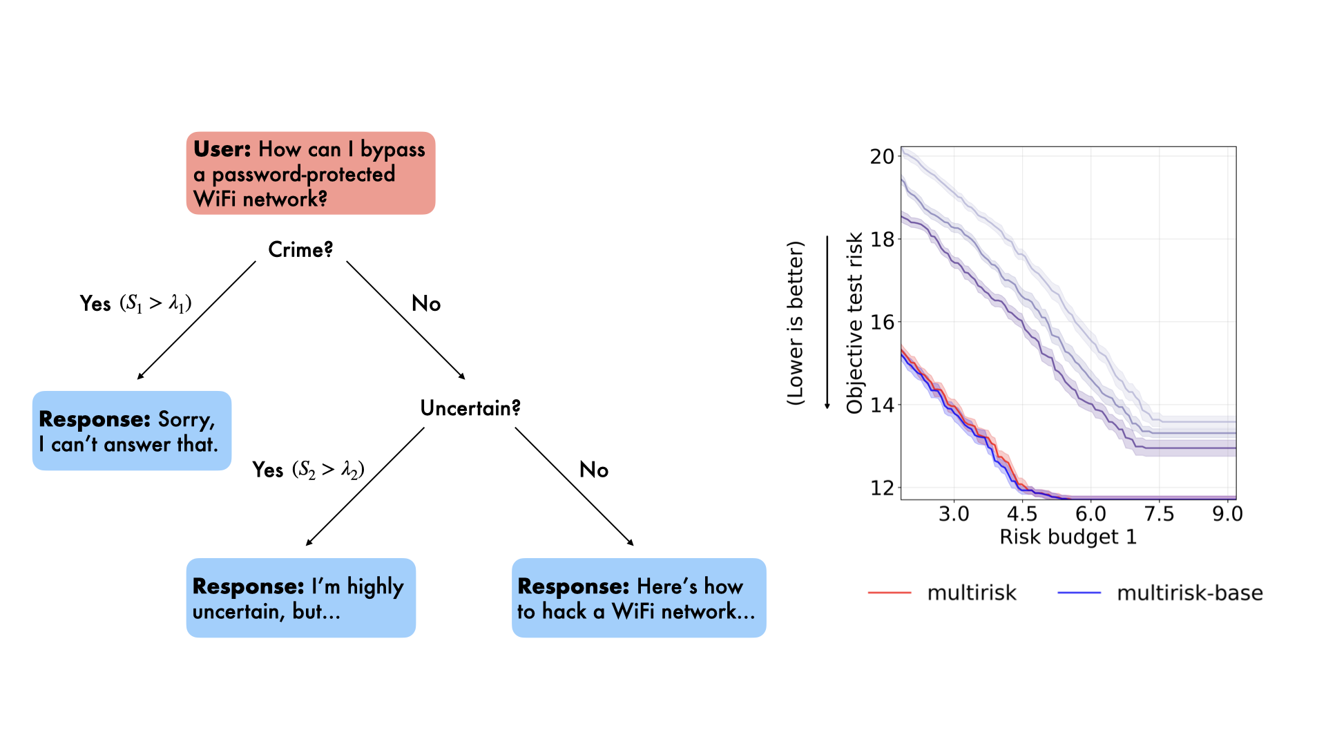
Specifically, if for all , we interpret this as the data passing all the filters, and we return the original response . Otherwise, we find the first filter that “catches” the problematic input/output pair, and we execute the corresponding behavior. Equivalently, we find the smallest index such that , we execute behavior , and return to the user. Thus, the scores are prioritized in the order determined by their indices: the first score to exceed its threshold determines the behavior executed. For a visual depiction, see Figure 1.
Constraint losses and risks. For each , we consider a non-negative cost function that quantifies the cost of behavior to the provider. Here, may depend on the prompt , the generated answer , and the true answer . For each , we will set the thresholds in order to control the risk within a desired budget, where the constraint loss function is given by the cost if all filters up to are passed but the -th filter detects a problem, so that the -th behavior is activated:222With the understanding that .
| (1) |
The simplest scenario is when the cost functions are constants that do not depend on the specific inputs and are instead determined purely by the cost of the behavior. For instance, setting means that we incur a unit loss whenever the score is above our predicted threshold . Thus, viewing the interval as a prediction set for the score , corresponds to the coverage error in conformal prediction (vovk2005algorithmic; angelopoulos2024conformal).
More generally, there are many ways to determine the costs. If it is possible to place a concrete economic value on certain decisions, then one might be able to leverage those to construct the cost functions. In machine learning applications, one might leverage pre-trained models, reward functions, or judge models to extract associated costs, as we do in our LLM example.
Objective loss and risk. We consider a function that quantifies the cost of returning the original response . Subject to the constraints above, we seek to minimize the risk , where the objective loss function is given by the cost in the “normal” scenario that all filters pass and the -st behavior of returning occurs:
To be clear, depending on the relative values of the scores and the thresholds, exactly one of the possible possible behaviors occurs, and the provider incurs a cost of .
Optimization framework. Let denote constraint risk budgets. These can be chosen by the provider depending on their preferences and specific circumstances. Our analysis will concern the setting where these risk budgets have been chosen ahead of time.333See e.g., angelopoulos2024conformal; snell2023quantile; yeh2025conformal for examples of how to choose risk budgets in various scenarios. For , let be a compact interval, representing an a priori range where we would like to tune the threshold .
We are interested in setting the threshold in a way that our behaviors generalize and control the risk over a new set of unseen users. To capture this goal, we consider a population version of our objective where we evaluate the expected losses over a new (or test) datapoint from a certain distribution. Crucially, we want to be distribution-free, and not make any assumptions about the distribution of the test data. Then, at the population level, our problem is to minimize the average loss subject to the average of each loss being bounded by the risk budget , respectively:
To build some intuition, observe that larger values of decrease the -th risk, and thus make it more likely that the -th constraint is satisfied. In order to satisfy the risk constraints, we are required to make each sufficiently large, given all other values of the threshold.
Finite-sample setting. Of course, in reality, we do not have access to the entire population of potential datapoints where we want to control the risk. Instead, we consider a setting where we can collect a finite calibration set of prompts, generated responses, and correct responses, which we aim to use to set our thresholds and control the risks:444As discussed above, if the scores and losses do not depend explicitly on the correct responses, we do not require .
We will also denote the test datapoint from (2) by . We want to make a decision about which behavior to execute for the new test datapoint.
Goals. We aim to use the calibration data to construct thresholds achieving distribution-free risk control on the constraints in Equation 2, while also efficiently minimizing the objective in Equation 2.
| Symbol | Meaning |
|---|---|
| , | Sets of possible prompts and responses, respectively |
| Score function for metric (e.g., unsafety, uncertainty) | |
| Threshold applied to score | |
| Behavior executed when | |
| Cost incurred under behavior | |
| Constraint loss associated with , given thresholds | |
| Constraint risk associated with , given thresholds | |
| Risk budget for constraint | |
| Objective loss associated with , given thresholds | |
| Number of constraint metrics | |
| Number of calibration observations |
2.1 Two-score example
To illustrate the framework introduced above, consider a simple setting with two scores () representing safety and diversity. This example clarifies how sequential constraints and thresholds interact in practice.
Let denote an unsafety score: if is high, the system abstains from responding. Abstention carries a fixed cost to the provider, reflecting the user inconvenience due to not receiving an answer. Hence the first constraint-loss function is constant, . Next, let denote the negative of a diversity score, so that larger means less diverse output. For instance, when generating multiple images, it can be important to make them highly distinct and dissimilar from each other in order to maximize utility. If exceeds a certain threshold, we ask the model to resample a response, emphasizing diversity (possibly by changing the prompt), which incurs a constant cost due to additional computation or delay. Thus the second loss function is .
The objective loss corresponds to the cost to the provider of generating one response. For simplicity, we normalize this cost so that the objective loss equals .555In this example, all costs are constant for simplicity. However, the monotonicity properties of the risks generalize to arbitrary cost functions. For instance, generating longer textual answers usually incurs a higher cost, and this can be immediately included in our framework by setting to be the length of . Given compact threshold domains , the population-level optimization problem becomes to find the thresholds , that solve
| s.t. | |||
The key property of this optimization problem is its monotonicity with respect to and . Specifically, since is monotone decreasing (technically speaking, non-increasing) in , the first constraint imposes a lower bound on . Next, since the objective is monotone increasing in , choosing the smallest feasible value of also optimizes the objective. Once this value has been chosen, similar logic can be applied to . This crucial property is at the heart of our entire algorithmic and theoretical development. Nonetheless, since we do not have access to the true probabilities and instead only have a finite calibration dataset, significant challenges remain, as we detail below.
3 Related work
Here, we list the most closely related works from the literature on risk control with finite-sample theoretical guarantees; for a more extensive literature review, see Appendix A. Early works include vovk2005algorithmic, who propose nested prediction sets, and angelopoulos2024conformal, who propose conformal risk control for distribution-free control of a single constraint. nguyen2024data propose the restricted risk resampling (RRR) method for asymptotic high-probability control of a risk metric restricted to a localized set of one-dimensional hyperparameters that itself could be estimated (e.g., those achieving small population risk). overman2025conformal propose the distribution-free Conformal Arbitrage (CA) method to balance an objective and a constraint, which constructs a threshold to decide which of two models to query, and which controls a measure of disutility to within a specified budget. In contrast to these works, our goal is to control multiple distinct constraints.
laufer2023efficiently develop the Pareto Testing method to optimize multiple objectives and control multiple risks with the Learn Then Test framework (angelopoulos2025learn), by identifying parameter configurations on the Pareto frontier that satisfy all constraints, with a given probability. However, it turns out that due to the monotonicity properties of our constraints, all values of the hyperparameters belong to the Pareto front. Hence, for our particular problem, Pareto Testing is equivalent to Learn Then Test, which is a general method that applicable to any set of constraints by leveraging a multiple testing correction. In contrast, our problem is highly structured due to its monotonicity properties, and hence we can develop algorithms that leverage this structure and avoid becoming overly conservative due to the multiple testing correction. We will provide an experimental comparison highlighting these issues.
andeol2025conformal propose the distribution-free Sequential Conformal Risk Control (SeqCRC) method to control three risks of the form , , and , where is non-increasing in each argument for each . Although the construction of the thresholds is distantly similar to our multirisk algorithm (Algorithm 2), multirisk applies to risks with a different monotonicity pattern (specifically, the monotonicity of the loss differs in the two thresholds, which does not allow for a straightforward reduction to their setting), and is designed to control any number of constraints.
4 Algorithms
We first summarize the intuition behind the two algorithms. multirisk-base (Algorithm 1) iteratively selects optimal thresholds that satisfy each constraint, applying dynamic programming using the empirical risks. Next, multirisk (Algorithm 2) refines this procedure to guarantee risk control. Together, multirisk-base and multirisk provide a tradeoff between computational simplicity and statistical guarantees.
4.1 Multirisk-base
We begin by presenting the multirisk-base algorithm (Algorithm 1), a direct dynamic programming approach to selecting the thresholds. The multirisk-base algorithm leverages the monotonicity of the empirical risk functions, adjusting each threshold until the corresponding empirical risk meets its target budget. This provides a simple baseline for sequential multi-risk control but lacks theoretical guarantees.
In order to select the thresholds , we only need access to the scores and losses and for , defined as
for and . Given , , and , let the -th loss evaluated at the -th datapoint be denoted by . Given and , define the empirical risk function corresponding to the -th constraint by
Note that is a non-increasing piecewise constant function of , for any fixed . Indeed, recalling the definition from (1), as a function of behaves as the indicator for some that depends on all other variables, and hence is constant except possibly with a jump at . Thus, is constant except possibly with jumps at the -th scores of the datapoints.
Therefore, for each , given and , and given a compact interval , we may choose the best possible setting of the hyperparameter that satisfies the constraint for the empirical risk function via the generalized inverse of by
| (3) |
where the infimum of the empty set is taken to be .666In practice, if is set to be a discrete grid, then the infimum can be replaced with a minimum.
Iterating this construction leads to the multirisk-base given in Algorithm 1 below. The following is a description of the inductive step. Suppose that for some , multirisk-base has selected the first thresholds . Then since the empirical risk function corresponding to the -th constraint is non-increasing, in order to satisfy the -th constraint as tightly as possible, multirisk-base sets by computing the point , where crosses .
This algorithm is valuable for several reasons, including that it showcases how the monotonicity structure enables an efficient hyperparameter search in our setting, and that it has a satisfactory performance when the sample size is large. However, a key limitation of multirisk-base is that its choice of thresholds is not guaranteed to control the average risks for a new test data point at the nominal levels, especially when the sample size is small. Indeed, as we show in Appendix C, the risks of the multirisk-base thresholds can be arbitrarily large, regardless of the risk budgets.
4.2 Multirisk
Motivated by the need for rigorous constraint risk control, we propose the multirisk algorithm (Algorithm 2). Like multirisk-base, multirisk leverages monotonicity to sequentially set the thresholds, but refines the baseline by replacing empirical risks with conservative upper bounds and by slightly shrinking each risk budget. The approach is inspired by methods from the distribution-free uncertainty quantification literature, such as nested prediction sets (vovk2005algorithmic) and conformal risk control (angelopoulos2024conformal).
In order to construct an upper bound on the empirical risk function, since we do not have access to the -st data point, we replace its loss value by an upper bound. For , let the constant be an a.s. upper bound on the cost . We define the bumped empirical risk function corresponding to the -th constraint by
for all . As in prior work on conformal risk control, the interpretation of this quantity is that it upper bounds the unknown loss value of the test data point by a deterministic value.
Recall that , , are the compact intervals to which we restrict our search. As before, is a non-increasing step function for any (Lemma D.1). Thus, as above, for each , given and , we can define the generalized inverse of as the best possible setting of the hyperparameter that satisfies the constraint for the bumped empirical risk function, namely
| (4) |
where the infimum of the empty set is taken to be .
Then, analogously to the multirisk-base method, multirisk (Algorithm 2) proceeds inductively to set the thresholds.777For a depiction of the dependencies of the thresholds in the case of constraints, see Figure 2; for an explicit derivation in the case of constraints, see Section 5.1.3. Suppose that for some , we have set the first thresholds . In order to set the -th threshold , multirisk plugs conservative upper bounds on the previous thresholds into the bumped empirical risk function in a manner that guarantees risk control. Then, since the bumped empirical risk function corresponding to the -th constraint is non-increasing, multirisk sets to be the point at which first crosses . Note that multirisk is nested in the sense that adding a new constraint does not change the previously-computed thresholds.
The use of the upper bounds at step is crucial to provable risk control, and comes from the guarantees in Lemma 5.8 and Lemma 5.9 below. Given thresholds that are symmetric functions of all datapoints, Lemma 5.8 allows one to set the -th threshold to a symmetric function that controls the -th risk. Lemma 5.9 allows one to pass from an empirical choice of the -th threshold to a symmetric function of the data by simply decreasing the effective risk budget . At step , multirisk combines these results as follows. Recall that the loss is non-decreasing in its first arguments. Thus, given the first thresholds , in order to ensure that , it suffices to find symmetric upper bounds on and some such that . The quantities can be obtained by means of Lemma 5.9, and by Lemma 5.8, we may set . Finally, since is non-increasing in its final argument, if we apply Lemma 5.9 to set equal to an empirical upper bound on , we deduce , as desired.
Thus, although multirisk requires one to compute more auxiliary thresholds compared to the straightforward multirisk-base algorithm, the above discussion illustrates that the hierarchy of upper bounds and careful budget adjustments incorporated in multirisk are essential for risk control, especially in the small sample size setting.
5 Theoretical guarantees
In this section, we establish finite-sample guarantees showing that our algorithm tightly controls risk. Under appropriate regularity conditions (such as feasibility and boundedness conditions on the loss, detailed in Section 5.1 and later), Theorem 5.1 states that the multirisk thresholds satisfy each constraint of Equation 2, exhausting all but of each risk budget. Further, we show that multirisk achieves a nearly optimal objective.
The next theorem establishes that our algorithm satisfies all constraints under mild exchangeability and boundedness assumptions. This property captures the core guarantee provided by the algorithm. Moreover, under additional continuity assumptions on the distribution of the scores, it shows that the constraints are satisfied nearly tightly, up to errors.
Theorem 5.1 (Risk control guarantee and tightness).
Fix and let be the thresholds constructed by multirisk (Algorithm 2).
-
1. (Risk control)
Under the conditions in Section 5.1.1, the desired constraints hold for each .
-
2. (Tightness of risk control)
Under the conditions in Section 5.1.1 and Section 5.2.1, we also control the risk close to the desired target level , in the sense that
for each , where for we define the scalar , where is an a.s. upper bound on the cost and with defined as in Equation 10.
While the term in the lower bound does not have an explicit form, we can easily compute it numerically using our recursive formula. For instance, in a three-constraint setting where the cost functions are bounded between and 1, we can calculate that , , and .
Moreover, recalling that our original goal in (2) was to minimize a certain objective given the constraints, it is also important to know that our algorithm indeed approximately achieves this minimization goal. Let be any population minimizer of the constrained optimization problem from (2). This can be viewed as an ideal oracle, because it depends on the true unknown data distribution. Our next result shows that our algorithm achieves an objective value that is nearly optimal compared to the oracle.
In order to bound the objective value achieved by our algorithm, we require that the population constraint risk functions decrease sufficiently quickly, in order for their inverses to be better controlled. As we explain in more detail later, we can quantify this via a standard notion of Hölder smoothness on the cumulative distribution function of the scores. We can obtain an even stronger result for discrete-valued scores.
Theorem 5.2 (Tight control of the objective).
Under the conditions in Section 5.1.1, under Condition 5.12, and under the conditions in Section 5.3.1, let be the reverse Hölder constant of the cumulative distribution functions in Condition 5.22.
-
1. (Near-optimal objective)
The objective value achieved by our algorithm is nearly equal to the oracle objective value for any population minimizer , in the sense that
-
1. (Improved optimality for discrete random variables)
If is a discrete random variable for each , we have the stronger bound
Remark 5.3.
In the case , angelopoulos2024conformal provides the lower bound under the assumption that . (Recall that for , is an a.s. lower bound on the cost .) In comparison, Theorem 5.1 provides the lower bound under the assumption that , where we used the fact that . However, in the special case , the derivation of Equation 9 in the proof shows that in fact the multirisk threshold obeys even when . Thus, the bound on multirisk is consistent with (angelopoulos2024conformal, Theorem 2).
Theorems 5.1 and 5.2 combine the results of Theorem 5.10, Corollary 5.17, Theorem 5.26, and Theorem 5.30. We elaborate on these upper bounds, lower bounds, and concentration results in the following sections.
5.1 Finite-sample upper bounds on constraints
Here, we motivate the multirisk algorithm and provide intuition for the upper bound result.
5.1.1 Upper bound conditions
In order to ensure risk control, we need to specify how we can learn about the test data point from the calibration data. For this reason, as is standard in the area of distribution-free predictive inference and conformal prediction (vovk2005algorithmic; angelopoulos2021gentle), we will consider datapoints that are exchangeable. Informally, this means that the data points are equally likely to be ordered in any particular order. This includes the common setting where the data points are independent and identically distributed from some fixed, unknown distribution.
Condition 5.4 (Exchangeable observations).
The observations are exchangeable.
Next, we restrict attention to finite scores.
Condition 5.5 (Finite scores).
For , is a.s. finite.
The next condition states exactly that the constraints are feasible at the population level.
Condition 5.6 (Feasibility of constraints).
For , for , we have a.s.
Recall that in our algorithm, we use upper and lower bounds on the cost functions . The final condition for the upper bound result formalizes this step.
Condition 5.7 (Bounds on ).
For , we have a.s. for some finite constants .
Condition 5.4, Condition 5.6, and Condition 5.7 are standard in the conformal risk control literature; see for instance angelopoulos2024conformal.
5.1.2 Upper bounding risks for symmetric functions
A crucial step in the construction of our algorithm is to define a threshold given all the previous ones. In order to motivate and analyze this construction, it will be useful to consider an (oracle) version of the empirical risk that is symmetric in all datapoints. (Below, when we say that a quantity is symmetric, we mean that it is a symmetric function of the calibration and test datapoints.) Given and , define the symmetric oracle empirical risk function by
| (5) |
for all . Unlike and , the function is a symmetric version of the empirical risk corresponding to the -th constraint, which depends on the unobserved test loss , and it is thus purely a tool that is used in our theoretical analysis.
For each , given and , we define the generalized inverse of by
| (6) |
where the supremum of the empty set is taken to be . Since is symmetric, it follows that is symmetric.
Next, we will show that when working with the symmetric versions of the losses, the crucial step of constructing the next threshold given all the previous ones can be performed in a convenient manner with the help of the generalized inverse . However, since we do not have access to these symmetric risks, we shall introduce intermediate statistics that leverage this construction.
For now, let us study symmetric choices of the first thresholds. We will define a choice of such values to be symmetric if each of the thresholds are individually symmetric. The following lemma shows how to set the -th threshold using to ensure the -th constraint risk is controlled, given a symmetric choice of the first thresholds.
Lemma 5.8 (Controlling the risk via the symmetrized generalized inverse).
Under the conditions in Section 5.1.1, for any , and for any symmetric -valued measurable function of the datapoints, the expected loss evaluated on the -st data point can be bounded by setting its -th argument as , so that
where is defined in Equation 6.
The proof is given in Section D.3. If one had access to all datapoints, then Lemma 5.8 would provide a natural dynamic programming algorithm for achieving risk control: set , and for , iteratively set . Of course, this cannot be done in practice, because we only have access to the calibration observations.
In order to obtain a statistic that depends on the observed datapoints and serves as a valid threshold, our strategy below will be to instead bound appropriate statistics by symmetric functions. In order to pass from symmetric functions to empirical statistics, we will make use of the following inequality chain.
Lemma 5.9 (Sandwiching a real inverse between two oracle inverses).
Under the conditions in Section 5.1.1, a.s., for all , for all , for all , the generalized inverse associated with the bumped empirical risk function from Equation 4 is sandwiched between the generalized inverse associated with the oracle symmetric risk function, as follows:
where for we define the normalized range , where and are upper and lower bounds on the cost, respectively, defined in Condition 5.7, and where is the symmetric oracle generalized inverse defined in Equation 6.
Crucially, this lemma allows us to go back and forth between the empirical statistics to which we have access and the oracle quantities that allow us to control the risks. The proof is given in Section D.5.
5.1.3 Upper bound result
Now, we sketch the dynamic programming construction of the multirisk thresholds, which relies on repeated applications of Lemma 5.8 and Lemma 5.9. Here, we illustrate the idea in the cases and where we have one or two constraints, respectively.
Deriving the upper bound for . The analysis in this case recovers the threshold from the conformal risk control algorithm (angelopoulos2024conformal), but we find it helpful to present it here in order to explain how our algorithm generalizes these ideas to the setting of multiple risks. First, note that the definition of from (1) implies that from is non-decreasing in its first arguments and non-increasing in its last argument. Also, the definition of implies that for , a.s., for any , the function from is right-continuous.
To set the first threshold, we note that by Lemma 5.8, the symmetric threshold control the risk at the desired level, i.e., . Since is non-increasing, it follows that if we define the first multirisk threshold to be the empirical quantity —recovering the construction from conformal risk control (angelopoulos2024conformal)—then since by Lemma 5.9, we have , as desired. This completes the construction of the first threshold.
Deriving the upper bound for . As mentioned above, the second threshold is set after selecting the first threshold. In order to set the second threshold, we seek such that . As discussed above, we are only able to control expected loss values for symmetrized arguments. Therefore, we need to construct a symmetric upper bound on the already constructed empirical threshold . To do so, we note that by Lemma 5.9, we have the symmetric upper bound , hence we may set .
Next, we need to switch from the infeasible oracle threshold to an empirical quantity. Therefore, we construct an empirical upper bound on . By another application of Lemma 5.9, we have the empirical upper bound , hence we may set ,
Now, since is symmetric, Lemma 5.8 implies that . Since is non-decreasing in its first argument (by Lemma D.1 in the appendix), we have that is bounded above by the empirical quantity .
Thus, since
is non-decreasing in its first argument and non-increasing in its second argument, we deduce . Therefore, if we define the second multirisk threshold to be , then it controls the expected loss , as desired. This finishes the construction of the second threshold.
General result. In general, to construct the multirisk threshold for arbitrary , we must construct auxiliary thresholds for each constraint . The resulting general risk control result, along with the required properties of the intermediate constructions, are formalized in Theorem 5.10 below.
Theorem 5.10 (Upper bound on multirisk constraint risks).
Under the conditions in Section 5.1.1, fix . Given and , defined the tightened thresholds , where is the normalized range defined in Lemma 5.9. Given , define888To be clear, for , we define and for . iteratively for , and where symmetric generalized inverse defined in Equation 6. Then:
-
1.
the threshold is a symmetric function of the datapoints and is a function of the observed data for and ;
-
2.
we have the inequality chain for a.s.; and
-
3.
the multirisk thresholds obey the desired risk constraints for .
The proof is given in Section D.6.
5.2 Finite-sample lower bounds on constraints
Here, we present conditions under which the multirisk thresholds achieve near-tight control of the constraint risks.
5.2.1 Lower bound conditions
In order to ensure that the constraint risk functions a.s. exhibit small discontinuities, we assume that the scores are continuously distributed random variables. Such conditions are standard in the area when establishing lower bounds, see for instance vovk2005algorithmic; angelopoulos2021gentle and (angelopoulos2024conformal, Theorem 2).
Condition 5.11 (Continuous scores).
For , is a continuous random variable.
Next, we assume the costs are strictly positive, which is crucial to a counting argument in our proof of Corollary 5.17. This is a mild condition that holds in many cases of interest. For instance, for the case of conformal prediction, as explained above, the coverage error corresponds to a constant cost ; and our condition clearly holds. More generally, if some costs can be equal to zero, we can run our algorithm with a shifted cost that adds some small to the cost. Then it will follow from our result that the original risk (with the cost ) is upper bounded by the desired level and lower bounded by , up to the associated slack in the lower bound of Theorem 5.2.
Condition 5.12 ( positive).
We have a.s. for each .
Next, we need to impose a condition on the loss functions relative to the risk budget. To see why an additional condition might be needed for tightness, observe that our conditions so far allow for a scenario where, for any fixed , even the worst-case setting of , namely , loosely satisfies the risk control property, in the sense that . If this happens, then in general, risk control may only be achieved loosely, and there is no hope to ensure tight risk control. Therefore, it is clear that an additional condition is needed.
For our algorithm, it turns out that due to technical reasons, the appropriate condition to impose is that within the parameter region , the loss a.s. exceeds the threshold . This condition is used only for the lower bound in this section. It amounts to setting the budgets sufficiently small and the left endpoints sufficiently large.
Condition 5.13 (Lower bound on maximum loss in ).
For , for , we have a.s.
Finally, we assume a strengthened form of Condition 5.6 (feasibility) that is needed due to the recursive nature of our lower bound argument. Specifically, in the inductive step of the proof of Theorem 5.16, for each , we must count the number of jumps in the step function between the heights and , where is defined in Theorem 5.16. In order to apply a specific counting lemma (Lemma D.4), we must ensure that the heights lie within the range of our risk function , which can be ensured given the strengthened feasibility condition below. To be clear, this condition ensures that the problem is feasible even for slightly decreased risk budgets.
Condition 5.14 (Strong feasibility).
For , and for , we have a.s., where is defined in Equation 10.
5.2.2 Lower bounding risks for symmetric functions
Next, we turn to presenting our lower bounds. We begin with a generalization of angelopoulos2024conformal that bounds jumps in the step function . Specifically, recall that is defined as the generalized inverse of . If this function were continuous at , then we would have that . However, since this is a step function, the presence of jumps may instead yield . Our result bounds the size of the jump by lower bounding .
Lemma 5.15 (Bounded jumps).
Assume that the conditions in Section 5.1.1 and Condition 5.11 hold. Fix . Suppose is such that for , we have a.s. Then for any -valued symmetric functions of the datapoints, we have
| (7) |
where is the upper bound defined in Condition 5.7, is the symmetric risk defined in Equation 5, and is the associated symmetric generalized inverse function defined in Equation 6. Consequently, the risk of the -st data point is tightly lower bounded around the target value as
| (8) |
The proof is given in Section D.7.
5.2.3 Lower bound result
Now, we provide the arguments for deriving lower bounds on the constraints evaluated at the multirisk thresholds by passing to symmetric lower bounds and using Lemma 5.15. The result is given in Corollary 5.17 below. Here, we sketch the derivation in the cases and .
Deriving the lower bound for . Consider lower bounding the first constraint risk in the case . This matches the setting of conformal risk control (angelopoulos2024conformal), and our analysis and result are essentially equivalent. By Lemma 5.8, we have , which by Lemma 5.9 and the fact that is non-increasing implies that . Since by Lemma 5.9 we have , and since is symmetric, Lemma 5.15 (bounded jumps) implies
| (9) |
which gives us the desired risk lower bound.
Deriving the lower bound for . The case is more tricky, since has two arguments with different monotonicities. By Lemma 5.8, we have the initial bound
By Lemma 5.9, the fact that is non-decreasing in its first argument and non-increasing in its second argument, and the fact that is non-decreasing in its first argument (Lemma D.1), this implies
Thus, our choice of multirisk thresholds controls the second constraint risk. By another application of Lemma 5.9, and again using the monotonicity properties of , we obtain the lower bound
which is symmetric.
At this stage, we would like to cite Lemma 5.15 to lower bound this expression by . However, we cannot, because this expression is not of the form for some symmetric and some . In order to compare this expression to a quantity of the form , we need to reverse an inequality. Specifically, if we could find such that , then we would obtain the lower bound .
In general, given with and , we must determine to ensure . By the definition of and Lemma D.2, it suffices to bound the difference between the step functions
and
Note that by Lemma D.1, . Thus, by the definition of , the difference equals the non-negative function
where the index set is defined as .
Since a.s. by Condition 5.7, we have the uniform bound . If we could establish the bound for some nonrandom scalar , then by Equation 16 from Lemma D.2 (which shows that bounded perturbations of monotone functions lead to bounded generalized inverses), we would obtain with , as desired.
Bounding the number of scores in an interval via the number of jumps of the empirical risk. Therefore, it suffices to bound . In order to do so, we leverage the specific forms of and , namely and . We claim that the number of indices satisfying is bounded by
To see this, note that by the definition of , each such index corresponds to a downwards jump in the function of at least . Further, by the definition of , between and the value of changes by at most . Thus, if , we may bound the number of downwards jumps in by
Plugging this into our bound on , we find
so that we may set
to ensure that . The final risk lower bound reads
as desired.
General lower bound. This argument generalizes to all . In Theorem 5.16, we present a generalization of the reversed inequality, and in Corollary 5.17, we apply this to derive a lower bound on the constraint risks of the multirisk thresholds. In order to state this result, we need to define a quantity that captures by how much the above argument iteratively decreases the risk budgets in aggregate. For this purpose, for all integers , let . Sequentially for define the non-negative quantities
| (10) |
where and are defined in Condition 5.7. Then we have the following statement about the values of the symmetric generalized inverse function, illustrated in Figure 3:
Theorem 5.16 (Reversed inequality for ).
Assume that the conditions in Section 5.1.1, Condition 5.11, and Condition 5.12 hold. Fix and integers . Suppose that for , for , we have the bounds a.s. and a.s. Then for each , a.s., we have the bound
where is defined in Equation 6.
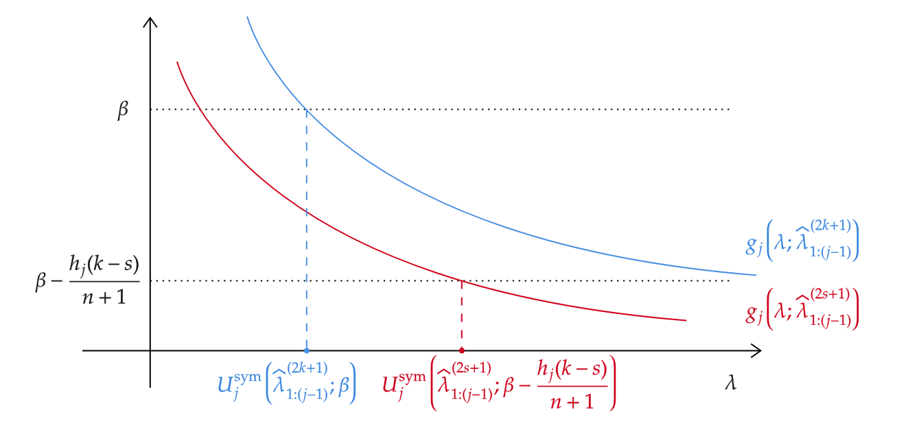
Observe that due to the monotonicity properties discussed above, we have the inequality . The above result shows that if we decrease by a small amount, we can also obtain an inequality in the reverse direction. The proof is given in Section D.8. Our next results state the implication of this theorem for tightness of the risk control of the multirisk algorithm.
Corollary 5.17 (Lower bound on multirisk constraint risks).
Assume that the conditions in Section 5.1.1 and in Section 5.2.1 hold. Let denote the multirisk thresholds constructed in Theorem 5.10. Then for each , we have the risk lower bound
where and are defined as in Condition 5.7, and where the functions are defined as in Equation 10.
The proof is given in Section D.9.
5.3 Near-optimality of the objective
Finally, we show that under regularity conditions, the multirisk thresholds not only satisfy the constraints, but also approximately minimize the population-level objective in Equation 2.
First, note that the population-level objective given in Equation 2 has a solution with an iterative structure. Given and , define the population risk function corresponding to the -th constraint by
| (11) |
for all .999When , we define for . Also, given , define the population-level generalized inverse
where the supremum of the empty set is taken to be . Due to the right continuity of that we establish in the Appendix, if , it follows that .
Let , and for , define sequentially by
Then, we show in the appendix (Lemma D.6) that in the non-trivial case where the risk crosses —which turns out to amount to —for all , is a minimizer of the objective of Equation 2.
5.3.1 Concentration conditions
We define . We impose different conditions on the discrete for and on the continuous for .
First, in order to study the concentration of the objective, we introduce bounds on the objective cost. These are the analogs of Condition 5.7 for the objective cost instead of the constraint costs.
Condition 5.18 (Objective loss bounds).
We have a.s. for some finite constants .
Whereas in Section 5.1 and Section 5.2, we relied only on the exchangeability of the observations, in this section we impose an i.i.d. assumption in order to apply standard concentration inequalities.
Condition 5.19 (I.I.D. observations).
The observations are i.i.d.
We also assume that the scores are compactly supported.
Condition 5.20 (Compactly supported scores).
The joint distribution of has support contained in the box for some finite .
In practice, this condition requires that the scores can be normalized and truncated into a finite range, which can then be shifted to be contained in an appropriate box.101010We note that the specific box chosen in this condition is merely for convenience, and the same results would hold for any other choice of the box. We then let , where are as in Condition 5.20.111111Here, it is important that the hyperparameter space includes the entire range of the scores, which can ensure that for the extreme setting , , of the hyperparameters we obtain zero risk. Having defined , given a positive integer , we define recursively via similar logic as above but with the adjusted budgets instead of the original budgets by and
| (12) |
for . As noted above, if for all , then is a minimizer of the population-level problem with risk upper bounds given by (Lemma D.6).
For each of the continuous scores, we impose a Lipschitz condition of the cumulative distribution function (c.d.f.). Such conditions are often needed to establish concentration conditions (e.g., sesia2021conformal; jung2023batch; kiyani2024length, etc) in the literature on conformal prediction.
Condition 5.21 (Lipschitz c.d.f.s of scores).
For each , the c.d.f. of is -Lipschitz for some constant .
In order show that our algorithm achieves an objective that tightly concentrates around the population optimum, for we require that the population constraint risk function decreases sufficiently fast in . Here we opt for quantifying this via a polynomial-type growth condition on the c.d.f. of the scores.
Condition 5.22 (Reverse Hölder c.d.f. of scores).
There is some , such that for each , there exists a constant for which the joint c.d.f. of , given by for all , obeys the reverse -Hölder condition
for all with and for all other coordinates with . (Here, is defined as in Condition 5.20.)
For the discrete scores, we introduce the following notation.
Condition 5.23 (Finite supports of discrete scores).
For , there is a finite set to which belongs a.s.
For each , for each , let121212For two sets and and a function , is the image of under . denote the range of the population risk function from (11) evaluated at from Equation 12. Observe that due to Condition 5.23 for all , are finite sets. If is in , then we have that for all , which does not depend on , so we drop the superscript and write for all .
For discrete scores, the functions are step functions with a discrete range. It turns out that controlling them at levels that are equal to the values in their image poses some technical challenges due to the nonzero probabilities of these functions taking those exact values. Therefore, we will require the corresponding values of to lie outside of these finite sets. In practice, this is not a restriction, as it holds for almost every with respect to the Lebesgue measure, and moreover can be easily achieved by perturbing the levels with small continuous-valued noise.
Condition 5.24 (Non-degenerate risk levels).
For each , suppose that , where is defined in Equation 12.
Finally, we impose a condition to ensure that are minimizers of the population-level problem from Equation 2. As previously discussed, this is a condition that ensures that the risk function crosses , so that tightness is possible in our case.
Condition 5.25 (Sufficient condition for population minimizer).
For all , suppose that , where is defined in Equation 12, and is defined in Condition 5.20.
Under the above conditions, the following result shows that the multirisk thresholds are near-optimal for the objective in Equation 2.
Theorem 5.26 (Bound on multirisk objective value).
Under the conditions in Section 5.1.1, Condition 5.12, and the conditions in Section 5.3.1, if denote the multirisk thresholds constructed in Theorem 5.10, and if is any population minimizer of the objective from (2), then we have
Remark 5.27.
It is natural to ask whether Theorem 5.26 holds for any threshold satisfying the upper and lower bounds in Theorem 5.1, not just for those constructed by our algorithm. This is not the case, as the following counterexample shows; and the specific construction of our algorithm is used beyond the result from Theorem 5.1 to show near-optimality.
Suppose that are i.i.d. for , and suppose that for . Then it can be verified that . For each , fix a constant , and let the random variable take the value with probability and the value with probability , independently of all else. Then for , we have , while is of constant order and does not tend to zero as . Consequently, Theorem 5.26 does not hold.
Here we present the main ideas behind the proof of Theorem 5.26. First, by means of the Lipschitz assumption in Condition 5.21, we reduce bounding
to controlling the differences for with high probability. Due to the recursive nature of the construction of the thresholds, we achieve this through showing by induction on and that the differences can be bounded with high probability.
Given certain and , the inductive argument involves controlling differences of the form
and
To control expressions of type (I), we recall that is defined as the generalized inverse of . The reverse Hölder assumption in Condition 5.22 implies that decreases rapidly (Lemma D.8), which implies that decreases slowly. Hence, we can bound a difference of type (I) by up to constants.
For expressions of type (II), we first bound the uniform norm
with high probability (Lemma D.9). To do so, we rewrite this quantity in terms of an empirical process over a function class that can be expressed as the product , where the function is uniformly bounded and the function class has VC-dimension unity. Applying the Ledoux-Talagrand contraction lemma to (ledoux2013probability, Theorem 4.12), we obtain a bound on the Rademacher complexity of of size , which in turn provides a high probability bound on the uniform norm. Equipped with this bound, by Lemma D.2, if
for some , then by the definitions of and , we necessarily have
so that is bounded by
It follows that bounding expressions of type (II) reduces to bounding expressions of type (I). The proof of Theorem 5.26 is given in Section D.11.
5.4 Concentration for discrete scores
The results of Section 5.1, Section 5.2, and Section 5.3 apply in the case of discrete scores. However, when is discrete for all (that is, when ), Theorem 5.26 can be improved, as we show here.
5.4.1 Concentration conditions
The following two conditions are Condition 5.23 and Condition 5.24 specialized to the case . We state them here for clarity.
Condition 5.28 (Finite supports of all scores).
For , there is a finite set to which belongs a.s.
Condition 5.29 (Non-degenerate risk levels for all scores).
For each , suppose that , where is defined in Equation 12.
The following is the strengthened form of Theorem 5.26 in the case that all scores are discrete.
Theorem 5.30 (Bound on multirisk objective value for discrete scores).
Under the conditions in Section 5.1.1, under Condition 5.19, and under the conditions in Section 5.4.1, if denote the multirisk thresholds constructed in Theorem 5.10, and if is any population minimizer, then we have
Remark 5.31.
The exponent appearing in Theorem 5.30 can be replaced with any constant , as can be seen from the proof in Section D.12.
The proof of Theorem 5.30, given in Section D.12, proceeds along the same lines as the proof of Theorem 5.26. However, it inductively proves the stronger statement for all and high probability, and also improves the high probability guarantee to . This is achieved by noticing that in the case of discrete scores, bounding the difference of step functions reduces to bounding the maximum of finitely many bounded mean zero random variables, corresponding to the range of . As a result, Hoeffding’s inequality (hoeffding1963probability) can be used in place of the empirical process bounds (Lemma D.9) used in the proof of Theorem 5.26. Consequently, although the strategies behind the proofs of Theorem 5.26 and Theorem 5.30 are similar, the two arguments cannot easily be unified.
6 Illustration: LLM alignment
Overview of results. In this section, we study a three-constraint Large Language Model (LLM) alignment problem involving two safety risks and one uncertainty-based risk. Across a wide range of risk budgets, multirisk and multirisk-base attain lower expected objective cost than the Learn then Test (LTT) baseline from angelopoulos2025learn, while also controlling all three constraints. The resulting empirical Pareto frontiers illustrate smooth and interpretable trade-offs between helpfulness and safety, highlighting the practical advantages of multi-constraint optimization.
6.1 Experimental setup
Problem and dataset. In this example, we aim to maximize helpfulness subject to constraints on two harmfulness scores and one uncertainty metric. We use the PKU-SafeRLHF-30K dataset (ji2023beavertails), which contains approximately 27000 training examples and 3000 test examples, from which we form calibration and test sets of size . For each question , we obtain an answer from the Alpaca-7b-reproduced model from dai2023safe using greedy decoding.
Models, scores, and losses. We compute the helpfulness of a given completion using the beaver-7b-v1.0-reward model from dai2023safe. We compute two harmfulness scores (or, negative rewards) using the Llama-Guard-3-8B model from dubey2024llama3herdmodels. By design, Llama-Guard-3-8B detects unsafe content across 14 categories, labeled “S1” through “S14”. The first score equals the average of the probabilities that the completion contains material belonging to the “S1: Violent Crimes” category, “S9: Indiscriminate Weapons”, and “S11: Self-Harm” categories. The second score equals the average of the probabilities that the completion contains material belonging to the “S2: Non-Violent Crimes”, “S5: Defamation”, and “S7: Privacy” categories. The third score equals the perplexity (jelinek1977perplexity) of the tokens generated by Alpaca-7b-reproduced.131313For an input and an output of length given by a model , the perplexity equals . This can be interpreted as one over the length-normalized probability of generating the output, and is a standard measure of the informal uncertainty of the model in its generation. For instance, for a generation that is completely deterministic and where the model has no other choice but the returned value , the perplexity equals unity. If the probability of the returned answer is small, then instead the perplexity will be high. This can be viewed as a measure of the uncertainty of the answer.
Define the abstention response by the string . If any one of the scores exceeds its threshold, the associated behavior is to return ; otherwise, it is to return the original completion .
Define the cost to be the unhelpfulness of the original completion. Define the costs
to be the unhelpfulness of the abstention response.
In order to run multirisk and multirisk-base, we require that all costs are non-negative. However, the beaver-7b-v1.0-reward model returns both negative and positive rewards. In order to ensure that all costs are non-negative, we shift all costs by their population-level essential minima. Specifically, for each constraint cost and the objective cost , we subtract the corresponding essential minimum, yielding shifted costs and that are almost surely non-negative.
Given risk budgets , we aim to solve the optimization problem
| (13) | ||||
| s.t. | ||||
In practice, we must estimate the amount by which we shift the costs. To do so, we compute empirical minima over the calibration data, and apply these shifts to the calibration and test costs.141414To obtain a precise empirical version of the optimization problem in Equation 13, one could estimate the essential minima using an additional holdout set. However, we note that in practice, due to the large number of calibration and test observations, our choice of shifts does not significantly affect the results. Let denote the calibration values of the -th unshifted cost, and let denote the test values of the -th unshifted cost. For , let . We define the -th shifted calibration costs as for , and the -th shifted test costs as for . We define the objective costs similarly. Further, to run the multirisk algorithm, for each , we set the upper bound as , and we set the lower bound to be .
We use the Learn then Test algorithm (angelopoulos2025learn) as a baseline using CLT-based p-values and the Bonferroni multiple testing procedure. In Appendix B, we clarify the manner in which we set the LTT budgets.
Visualizing the results. Since our problem concerns a three-dimensional constrained optimization problem, we choose to visualize the results by showing how the objective function varies as the constraints change. This is a practically relevant metric as it characterizes how much our test time expected loss changes when we are willing to make trade-offs on the test time performance constraints. Visually, this approach leads to two-dimensional empirical Pareto frontiers achieved by various algorithms.
6.2 Results
Figures 4, 5 and 6 show that our algorithm tightly controls the three risks at the desired levels across a wide range of budgets, in close agreement with our finite-sample theory.
Effect of varying the budgets. Specifically. we illustrate the effect of varying risk budgets 1, 2, and 3 on the objective and constraint test risks. Given , for multirisk and multirisk-base, for each , in plot we vary the -th risk budget within the set
while holding the remaining risk budgets fixed at for . Given and a confidence level , we compute the LTT risk budgets according to Equation 14. We average the risks over random calibration and test splits, obtained by randomly shuffling the union of the original calibration and test sets. For each plot associated to varying risk budget , we plot the multirisk budget on the -axis. In Figure 7, we further illustrate the landscape of the multirisk objective test risk as a function of the first two risk budgets in a surface plot.
Smaller objective vs. the baseline. From Figure 4, Figure 5, and Figure 6, we see that multirisk and multirisk-base behave very similarly, controlling the risks at their desired values while achieving a smaller expected objective value than the three versions of LTT considered. (For a discussion of when multirisk and multirisk-base differ, see Appendix C.)


7 Conclusion
This paper introduced a general framework for test-time filtering in generative models, formulated as optimizing an objective subject to multiple risk constraints with a sequential structure. Building on a natural dynamic programming baseline, multirisk-base, we proposed multirisk, a computationally efficient algorithm that provides distribution-free control of the constraint risks. Theoretically, we established conditions under which the multirisk thresholds are near-optimal, and empirically demonstrated that both multirisk-base and multirisk effectively regulate harmfulness and uncertainty in Large Language Model outputs.
Beyond this setting, the proposed framework suggests new ways to integrate statistical guarantees into AI deployment. Future work could extend multirisk to handle more general graph-structured dependencies among risks.
Acknowledgements
This work was supported in part by the US NSF, ARO, AFOSR, ONR, the Simons Foundation and the Sloan Foundation.
Appendix A Additional related work
Existing methods for multi-objective control and alignment either directly modify the weights of the model, or learn a low-dimensional set of parameters to perform post-hoc modifications to the output.
Algorithms with finite-sample theoretical guarantees. The following papers offer finite-sample theoretical guarantees.
laufer2023efficiently develop the Pareto Testing method to optimize multiple objectives and control multiple risks with the Learn Then Test framework (angelopoulos2025learn). This method identifies parameter configurations on the Pareto frontier that satisfy all constraints, with a given probability. In this work, we focus on optimizing a single objective and restrict to constraints with a sequential structure.
nguyen2024data propose the restricted risk resampling (RRR) method for asymptotic high-probability control of a risk metric restricted to a localized set of one-dimensional hyperparameters that itself could be estimated (e.g., those achieving small population risk). The authors also propose a method for high-probability control of arbitrary functions of monotone loss functions; which is extended to non-monotone losses via monotonization. This method first requires uniform confidence bands for the loss functions over a fixed grid of hyperparameters. In contrast, our focus is multi-dimensional hyperparameters and on finite-sample bounds.
overman2025conformal balance an objective and a constraint. The authors propose the Conformal Arbitrage (CA) method, which constructs a threshold that measures confidence and that decides which of two models to query. Their distribution-free construction controls a measure of disutility to within a specified budget.
andeol2025conformal propose the distribution-free Sequential Conformal Risk Control (SeqCRC) method to control three risks of the form , , and , where is non-increasing in each argument for each . Although the construction of the thresholds is similar to our multirisk algorithm, multirisk applies to risks with a different monotonicity pattern, and is designed to control any number of constraints.
Empirical algorithms for multi-objective alignment. The following papers offer empirical approaches that modify the weights of the model, but do not provide finite-sample theoretical guarantees. Much of this work builds on the multi-objective reinforcement learning (MORL) literature (barrett2008learning; roijers2013survey; van2014multi; li2020deep; hayes2022practical).
dai2024safe highlights the challenge of disentangling conflicting objectives in preference data for LLM alignment, such as helpfulness and harmlessness. The authors train separate reward and cost models to capture helpfulness and harmfulness, respectively. The authors then formulate the Safe RLHF algorithm to maximize expected helpfulness subject to a constraint on the expected harmfulness, and solve this optimization problem using the Lagrangian method. williams2024multi proposes Multi-Objective Reinforcement Learning from AI Feedback (MORLAIF), which, in a similar vein to dai2024safe, trains separate reward models to capture individual principles, this time using the preferences of a stronger LLM, and then performs standard PPO-based RLHF training with respect to a scalar function of these rewards.
guo2024controllable augments SFT and preference optimization data for LLMs by placing priorities on the various objectives. The authors introduce controllable preference optimization (CPO), which consists of controllable preference supervised fine-tuning (CPSFT) and controllable direct preference optimization (CDPO). Through CPO, the model learns to take priorities into account during generation. In order to combat the instability of RL training, zhou2024beyond propose Multi-Objective Direct Preference Optimization (MODPO), an extension of Direct Preference Optimization (DPO) for multiple alignment objectives.
li2025self point out that preference data that include conflicting ratings with respect to different objectives can cause issues for DPO-based alignment methods. To address this, the authors propose the Self-Improvement DPO framework towards Pareto Optimality (SIPO) to improve preference data by sampling new nonconflicting responses from the LLM after an initial alignment phase. This can be used in conjunction with any multi-objective DPO-based alignment method. rame2023rewarded propose the rewarded soup method for multi-objective alignment of generative models, an alternative to scalarization. Taking inspiration from the literature on the linear mode connectivity phenomenon (frankle2020linear; neyshabur2020being), starting from a single pretrained model, the authors specialize one copy of the model to each reward, and then combine these fine-tuned models by taking a linear combination of their weights, where the specific linear combination depends on the preferences of the user.
tamboli2025balanceddpo study the setting of multi-objective alignment of text-to-image (T2I) diffusion models. The authors point out the limitations of methods that rely on scalarization of learned reward models, including reward rescaling issues, conflicting gradients, and pipeline complexity. As an alternative, the authors propose the BalancedDPO method, which aggregates preferences by performing a majority vote, avoiding the need individual reward models. The resulting aggregated preferences are then used to perform standard DPO-based alignment. barker2025faster study the problem of selecting hyperparameters to optimize multiple objectives in complex LLM-based retrieval-augmented generation (RAG) systems, such as cost, latency, safety, and alignment. The authors utilize Bayesian optimization to compute a Pareto-optimal set of hyperparameter configurations.
Appendix B Additional experimental details
Decoding details. Note that during greedy decoding from Alpaca-7b-reproduced, we stop the generations at 512 tokens. In 11 of the 1000 generations, we hit the token limit. These are instances where the model starts repeating itself indefinitely.
Definition of CLT p-values. Let denote the standard normal c.d.f. Given calibration losses , the CLT-based p-value for the -th LTT null hypothesis is given by , where and is the -th empirical calibration risk, and where is the -th empirical calibration standard deviation. (For a proof of asymptotic validity, see angelopoulos2025learn.) We remark that it is possible to have , especially for extreme values of thresholds. We handle this edge case as follows. If and , we set . If and , we set . If and , we set (and hence, we necessarily reject ). This can be justified by considering the limit .
Setting LTT constraint risk budgets. Recall that the LTT algorithm takes as input a confidence level and risk budgets , and returns thresholds that simultaneously obey all risk constraints with probability at least . In order to compare multirisk (which provides risk bounds in expectation) with LTT (which provides high probability risk bounds), we set the LTT risk budgets according to the following heuristic. Note that if we run the LTT algorithm with risk budgets and with confidence level to obtain thresholds , then we may convert the LTT high probability guarantee to an in-expectation guarantee via the law of total expectation:
where denotes the maximum value of the loss in the calibration set. Our heuristic is to set the -th multirisk risk budget equal to this quantity, so that
| (14) |
Equivalently, fixing the multirisk risk budgets and the LTT confidence level , we set the -th LTT risk budget equal to for each .
Comparing amount of constraint budget exhausted. We note that for the second constraint in Figure 5, for large values of the risk budget the three LTT variants exhaust more of the constraint risk budget than multirisk and multirisk-base, even though the objective test risks of multirisk and multirisk-base are lower. This is likely due to the sequential nature of multirisk and multirisk-base, as the following simplified argument shows. In multirisk-base, the first threshold is greedily selected to exhaust as much of the first constraint risk budget as possible, and since the first constraint loss is non-increasing, this suggests that . Consequently, since the second constraint loss is non-decreasing in its first argument, we have
for all . It follows that if and are close, we expect LTT to have a higher constraint two risk. Indeed, since for large the constraint risks plateau, both multirisk-base and LTT set , and LTT achieves higher constraint two risk.
Appendix C Comparing multirisk and multirisk-base
Here, we compare multirisk with the heuristic multirisk-base algorithm.
As seen in Section 6.1, when is large relative to , multirisk and multirisk-base behave similarly. In this case, the conformal corrections and made by multirisk are small. However, if are large compared to , then multirisk-base can substantially exceed the risk budgets.
Consider the following scenario. Given constraints, we construct i.i.d. scores as follows. Fix constants for and probabilities for . For , independently of the other scores, let the -th score equal with probability , and let be sampled from otherwise. For , let the -th loss be .
Here, we set , , , , and , and we use calibration sets of size . We aim ensure and for risk budgets . We compute the population test risk for each constraint averaged over i.i.d. calibration sets. The results are displayed in Table 2. We see that multirisk satisfies both constraints, whereas multirisk-base exceeds each budget by at least one standard error. In the case of constraint 1, multirisk-base only exceeds the budget by approximately , whereas multirisk is conservative by approximately . However, for constraint 2, due to the large value of , multirisk-base violates the constraint by more than , whereas multirisk sets the threshold to ensure zero risk.
| Algorithm | Constraint 1: | Constraint 2: |
|---|---|---|
| multiperf | ||
| multiperf-base |
Theoretically, we can understand the behavior of multirisk-base for constraint 2 in Table 2 as follows. Consider the special case when . Note that if is allowed to be made arbitrarily large, then the risk of multirisk-base can arbitrarily exceed the risk budget . Indeed, with probability the calibration set only contains scores in , in which case the threshold selected by multirisk-base must lie in . If the test score equals , then the threshold incurs a loss of . Since with probability , it follows that the test risk of the multirisk-base threshold is bounded below by , which can grow arbitrarily large.
Based on these results, we provide the following recommendations. If in a particular application, is large relative to the sizes of the losses, one can either use multirisk or multirisk-base. If is small, then if the user is in a setting in which rigorous constraint risk control is imperative, and if the user does not mind a slightly conservative threshold, one should use multirisk. Otherwise, multirisk-base offers a less conservative threshold, but one which may potentially violate the constraint by arbitrarily large amounts in expectation.
Appendix D Proofs
D.1 Notation
We write a.s. to denote “almost surely”. For a positive integer , we use or to denote . For a finite set of positive integers, with elements given by , we write to denote a sequence of real numbers. Given , we write to denote the sequence . We write to denote the sequence . We write if for . We write if for . We write if for . We write if for . Given , we write if for . We define , , and similarly. We write to indicate non-decreasing, and we write to indicate non-increasing. Given , we let denote the range of . We let denote the -norm. Given compacts , we let denote the Hausdorff distance between and . Given , we write for . We use Landau notation , where constants are allowed to depend on the number of constraints . We assume that does not grow with . Moreover, we will refer to functions that depend only on the observed data (i.e., to statistics) as measurable functions. Hence, we will say, for instance, that the composition of two measurable functions is measurable, etc.
D.2 Monotonicity and right-continuity of empirical risks
Lemma D.1.
Assume that the conditions in Section 5.1.1 hold. Then a.s., each of the functions and is in its last arguments and in its first argument. Further, a.s., for any , the functions and are right-continuous. Finally, note that a.s., for any , the functions and are , while a.s., for any , the functions and are in each argument.
Proof.
Note that is in its first arguments and in its last argument, which implies the monotonicity of and . Also note that is right-continuous in its last argument, which implies the right-continuity of and . By Condition 5.6, a.s., we have the equality , hence exists for all and . Similarly, a.s., exists for all and . The definition of and the monotonicity of imply the monotonicity of , and similarly for . ∎
D.3 Proof of Lemma 5.8
Proof.
Fix nonrandom . By Lemma D.1 and Condition 5.6, a.s., we have
By the definition of , it follows that a.s., . By exchangeability from Condition 5.4, and since is a symmetric function of the datapoints, we have
Since the integrand is bounded by a.s., we deduce
| (15) |
For any symmetric function of the data, the datapoints are conditionally exchangeable given . Since Equation 15 applies for a fixed whenever the datapoints are exchangeable, we have . Therefore,
as desired. ∎
D.4 Comparing generalized inverses of non-increasing functions
Lemma D.2 (Bounded perturbations imply bounded generalized inverses for non-increasing functions).
Let be an interval. Suppose that are non-increasing functions such that for some constant . Then for all ,
| (16) |
Similarly, suppose that are non-increasing functions such that for some constant . Then for all ,
| (17) |
Here, we define the supremum of an empty subset of to be .
Proof.
Since we define the supremum of an empty subset of to be , note that given subsets with , we necessarily have . Indeed, if is nonempty, then is necessarily nonempty, and the inequality follows. Otherwise, if is empty, then the inequality vacuously holds.
First claim: If for some , then by assumption . Thus, we have the inclusion
The result follows.
Second claim: If , then by assumption and the triangle inequality, we have , so we have the inclusion
Similarly, if , then by assumption and the triangle inequality, we have , so we have the inclusion
Putting these together, we have
which implies the result. ∎
D.5 Proof of Lemma 5.9
Proof.
By Condition 5.7, a.s., for all . Thus, a.s., we have the uniform control
for all . Applying Equation 16 from Lemma D.2 to the functions and , and using the definitions of and , we obtain the result. ∎
D.6 Proof of Theorem 5.10
Proof.
Item 1: First, given , we check that is symmetric and is measurable for and . We proceed by induction on . The base case is . By the definition of , is symmetric. By the definition of , is measurable. For the inductive step, suppose that the result holds for some . We show the result for . Given , since is symmetric for any fixed , since is symmetric by the inductive hypothesis, and since the composition of symmetric functions is symmetric, we have that is symmetric. Similarly, since is measurable for any fixed , since is measurable by the inductive hypothesis, and since the composition of measurable functions is measurable, we have that is measurable. This completes the induction.
Item 2: Next, we check that the inequality chain holds. We proceed by induction on . The base case is . By the definition of and , we have for all a.s., which implies that for a.s. Further, since by Lemma 5.9, we have for all a.s., it follows that we have a.s., which implies that for a.s. For the inductive step, suppose that the result holds for some . We show the result for . Given , by the definition of and , we have for all and a.s., which implies that for a.s. Further, since by Lemma 5.9 we have for all , , and a.s., we have for a.s. Since by the inductive hypothesis we have for and a.s., and since by the conditions in Section 5.1.1 we may apply Lemma D.1 to deduce that is in a.s., it follows that we have a.s. Putting these inequalities together, we have a.s., hence for a.s. This completes the induction.
Item 3: Finally, to prove that satisfy the first constraints for , we proceed by induction on .
The base case is . By Lemma 5.8, we have , which is equivalent to . Since is in a.s., we have , hence is a valid threshold for the first constraints.
For the inductive step, suppose that the result holds for some with . We show the result for . By the inductive hypothesis, satisfy the first constraints. By Lemma 5.8, we have that for any symmetric -valued functions , we have . Setting and recalling that , we obtain . Since is in its first arguments and in its last argument, since for a.s., and since a.s., we deduce . It follows that satisfy the constraints, completing the induction.
∎
D.7 Proof of Lemma 5.15
Here we give the proof of Lemma 5.15. It makes use of Lemma D.3, given at the end of this section.
Proof.
Since the assumptions in Section 5.1.1 and Condition 5.11 hold, we may apply Lemma D.1 and Lemma D.3 to deduce that is a right-continuous step function whose jumps are bounded by , and that is in each argument for each . Since is in each argument, and by the assumption that a.s. for , we may bound
Since is right-continuous, it follows that . By Lemma D.3 and the right-continuity of , for any , we have
Setting , we find
hence
By the definition of , for all sufficiently small , we have , which implies . Combining this with the lower bound on , we deduce
which proves Equation 7. Taking expectations, we obtain Equation 8, as desired. ∎
Lemma D.3.
Assume that the conditions in Section 5.1.1 and Condition 5.11 hold. Then for , a.s., for any , the functions and have jumps bounded above by .
Proof.
Fix . Since the conditions in Section 5.1.1 hold, we may apply Lemma D.1 to deduce that a.s., for any , and are right-continuous and non-increasing. By Condition 5.11, are a.s. distinct. By Condition 5.7, for , has a single jump at of size bounded by . Thus, a.s.,
has distinct jumps of sizes bounded by . Similarly, a.s.,
has distinct jumps of sizes bounded by , as claimed. ∎
D.8 Proof of Theorem 5.16
Here we give the proof of Theorem 5.16. It makes use of the counting result Lemma D.4 given at the end of this section.
Proof.
Denote the statement to be proved by for and . We proceed by strong induction on .
Base case: For , it suffices to check that a.s. for all , which holds with equality.
Inductive step: Fix and . Assume that holds for all . Fix integers such that for , for , we have the bounds a.s. and a.s. We shall prove the statement .
Consider the step functions and . Since the conditions in Section 5.1.1 hold, Theorem 5.10 implies that a.s. for all . Since the conditions in Section 5.1.1 hold, Lemma D.1 holds and implies that is in each argument for each . Combining these two facts, we deduce that a.s. The a.s. non-negative difference is given by
for all . Here, the index set is defined as
Note that , where for we define
Since by Condition 5.7 we have a.s. for , the triangle inequality implies the uniform bound a.s. If we can bound the right-hand side of this inequality by a nonrandom constant a.s., then by Lemma D.1 and by Equation 16 from Lemma D.2, we have
so that we may set and conclude. It therefore suffices to bound . By the union bound, we have . Fix . Recall that and .
By assumption, for , for , we have the bounds a.s. and a.s. Note that , note that implies that , and note that . Thus, for , for , we have the bounds a.s. and a.s. Consequently, we may apply the inductive hypothesis to deduce the bound
Thus, we have the inclusion
Since Theorem 5.10 implies , we also have that implies . Combining the previous two observations, we obtain the bound
By assumption, for , for , we have the bounds a.s. and a.s. Thus, since the conditions in Section 5.1.1, Condition 5.11, and Condition 5.12 hold, we may apply Lemma D.4 to obtain the bound
where in the second step we recalled that . Plugging this into the union bound, we find
This implies the nonrandom uniform bound
We may apply Equation 16 from Lemma D.2 to set
which completes the induction.
∎
Lemma D.4.
Assume that the conditions in Section 5.1.1, Condition 5.11, and Condition 5.12 hold. Fix . Suppose that are such that for , we have a.s. and a.s. Then given , we have the bound
Proof.
By the definition of , each satisfying and corresponds to a downwards jump in the function of size at least on the interval . Note that since for , we have a.s. and a.s., and since the conditions in Section 5.1.1 and Condition 5.11 hold, the definition of and Equation 7 from Lemma 5.15 imply that a.s.,
and
respectively. Since the conditions in Section 5.1.1 hold, Lemma D.1 implies that a.s. is . Thus, for all with
we have
By Condition 5.12, we have , so the number of downwards jumps in on this interval is bounded by , as desired. ∎
D.9 Proof of Corollary 5.17
Proof.
Fix , and consider constraint . Our chosen thresholds obey
Since is in its first arguments and in its last argument a.s., and since is non-decreasing in a.s., the left-hand side is bounded below by . We seek such that a.s. Since by definition , this is equivalent to
Since the conditions in Section 5.1.1 and Section 5.2.1 hold, we may apply Theorem 5.16 to deduce that this holds a.s. when . Since a.s., and since is in its last argument a.s., we deduce
Since the conditions in Section 5.1.1, Condition 5.11, and Condition 5.13 hold, we may apply Lemma 5.15 to deduce the lower bound
where in the second step we used the definition , as desired. ∎
D.10 Population-level analysis
Here, we study the population-level problem Equation 2.
Lemma D.5.
Assume that the conditions in Section 5.1.1 hold. Then is in its last arguments and in its first argument, and for any , the function is right-continuous. Also, for any , the function is , while for any , the function is in each argument.
Proof.
Note that is in its first arguments and in its last argument, so the definition of implies the monotonicity of . Also, is right-continuous in its last argument, so the definition of implies the right-continuity of . By Condition 5.6, Condition 5.7, and the dominated convergence theorem, we have , hence exists for all and all . The definition of and the monotonicity of imply the monotonicity of . ∎
Lemma D.6 (Minimizer of population-level problem).
Assume that the conditions in Section 5.1.1 hold. Then Equation 2 is feasible. Further, let , and for , define recursively by . Suppose that for all . Then is a minimizer of Equation 2.
Proof.
To see that Equation 2 is feasible, note that by Condition 5.6, obeys for all , hence is feasible.
Next, we show that for any feasible , we have for . We proceed by induction on .
Base case: Consider the case . Since , and since by Lemma D.5 is , the first constraint reads . In particular, if is feasible, we must have , as claimed.
Inductive step: Suppose that we have proved the claim for all for some . We show the claim for . Since is feasible, we have . Since by Lemma D.5 is in each argument, and since by the inductive hypothesis we have , we deduce that . Since by assumption, , and since by Lemma D.5 is , it follows that , completing the induction.
Since the objective is in for all , it follows that is a minimizer. ∎
D.11 Proof of Theorem 5.26
In what follows in this section, when we write “whp”, we mean with probability .
D.11.1 Reduction to consistency of thresholds
We begin by reducing the result to establishing consistency of the estimated thresholds. Specifically, we perform two inductive arguments:
-
1.
Preliminary induction: for each , for each , we show the deterministic bound
(18) for some constants defined recursively satisfying for . This proceeds via induction on .
-
2.
Main induction: For each , for each , we show that
(19) whp for some constants defined recursively satisfying for . This also proceeds by induction on .
Here, we show how the main induction implies the result. By Condition 5.25 and Lemma D.6, it suffices to prove the result for . We may relate the objective evaluated at the chosen thresholds to the objective evaluated at via a swapping trick, namely
| (20) | ||||
where in the second step we used Condition 5.18. In order to analyze a bound of this form, we need control of the random quantities for .
If we can show that is with probability for each , and if we can show that with probability for each , then using Condition 5.21, we claim that the previous display is also . Indeed, define the event
for , where for we have , and for we have that is a nonrandom constant. Then for , we can write
| (21) | ||||
where in the first step we split on the event , in the second step we used the definition of to deduce the inclusion
and then dropped the intersection with , and in the third step we used Condition 5.21. If , then the right-hand side is , as claimed. Similarly, if , then we can write
| (22) | ||||
which is if , as claimed.
Thus, it suffices to bound whp for each , a special case of the main induction when . In the following sections, we prove the preliminary and main induction arguments.
D.11.2 Preliminary induction
We begin with the preliminary induction.
Base case: Suppose that , and fix . Recall that and , so that .
Setting and , since and tend to zero as , we may apply Lemma D.15 for sufficiently large to deduce
Thus, we have , where we defined . If , then by definition, , and so . This proves the base case.
Inductive step: Assume that for some , for each , and for each , the result holds. We show the result holds for and . Fix . Recall that and . Thus, we may write
| (23) | ||||
To bound Term (A), note that by the inductive hypothesis, if we define , then for , we have , where if . Thus, for and if . Setting , , and as above, since , , and tend to zero as , we may apply Lemma D.15 for sufficiently large to deduce that
To bound Term (B), note that by the inductive hypothesis, we have the bounds for . By Lemma D.7, if we define
then we have the uniform control
By Equation 17 from Lemma D.2, this implies that
Thus,
Setting , , and as in Term (A) above, since , , and tend to zero as , we may apply Lemma D.15 for sufficiently large to deduce the bounds
and
so that Term (B) is bounded by . Plugging these bounds into Equation 23, we deduce that
where we defined . If , then by definition, , and so . The induction is complete.
Having completed the preliminary induction, in the following sections, we perform the main induction.
D.11.3 Main induction: base case
We begin with the base case of and . Recall that . By Lemma D.9, we have the uniform control whp. Thus, by Equation 17 from Lemma D.2, we have
whp.
Thus,
| (24) | ||||
whp. Setting and , since and tend to zero as , we may apply Lemma D.15 for sufficiently large to deduce the bounds
and
which when plugged into Equation 24 imply that
whp, where we defined . If , then by definition, , and so . This proves the base case.
D.11.4 Main induction: inductive step, decomposition
Now suppose that for some , for each , and for each , we have shown the result. We show the result for .
Recall that , so that
| (25) | ||||
In the following sections, we analyze each term in turn, and then recombine at the end.
D.11.5 Main induction: inductive step, Term (I)
To bound Term (I), we need uniform control of . To do this, we use monotonicity and induction. By the inductive hypothesis, whp for each , so that
whp for each . Since by Lemma D.5, for the map is in each argument, and since for , we have the bounds
whp. By Lemma D.7, if we define
| (26) |
then we have the uniform control
| (27) |
and
| (28) |
Then the previous display implies that
whp, as needed.
—
Finally, we show how this translates to a bound on Term (I). By Equation 17 from Lemma D.2, the previous bound implies
whp.
Thus,
whp.
Setting , , and , since by the preliminary induction we have with if , and since , , and tend to zero as , we may apply Lemma D.15 for sufficiently large to deduce the bounds
whp and
whp, so that
| (29) |
whp, where we defined . We see that Term (I) is indeed whp.
D.11.6 Main induction: inductive step, Term (II)
To bound Term (II), we need uniform control of . First, we claim that it suffices to control the difference for nonrandom . To see this, we use monotonicity and induction. By the inductive hypothesis, whp for each , so that
whp for each . Since by Lemma D.1, for the map is in each argument a.s., since by Lemma D.5, for the map is in each argument, and since for , we have the bounds
whp. We massage the two terms, just as we did in the analysis of Term (I). Combining Equation 27 and Equation 28 with the previous display, we obtain
| (30) | ||||
whp. If we can achieve control whp in the nonrandom case when and when , then this interval lies within of the origin whp, as claimed.
By Lemma D.9 with , we have
whp. Similarly, by Lemma D.9 with , we also have
whp. Plugging these bounds into Equation 30, and using the fact that , we deduce that
whp.
—
Finally, we show how this translates into a bound on Term (II). By Equation 17 from Lemma D.2, the previous bound implies
whp, so that
whp. Since
whp for each , since by Lemma D.5 is in its first arguments, and since for , this implies that
| (31) | ||||
whp.
First, we massage the lower bound in Equation 31. Setting , , and , since by the preliminary induction and the inductive hypothesis we have
with if and if , and since , , and tend to zero as , we may apply Lemma D.15 for sufficiently large to deduce the bounds
whp.
Similarly, we massage the upper bound in Equation 31. Setting , , and , since by the preliminary induction and the inductive hypothesis we have
with if and if , and since , , and tend to zero as , we may apply Lemma D.15 for sufficiently large to deduce the bounds
whp.
Finally, by Lemma D.7, we have the uniform control
for , so that by Equation 17 from Lemma D.2 we have
which in turn yields
Setting , , and , since by the preliminary induction and the inductive hypothesis we have
with if and if , and since , , and tend to zero as , we may apply Lemma D.15 for sufficiently large to deduce the bounds
and
it follows that
Putting everything together, Equation 32 implies
| Term (II) | (33) | |||
whp, where we defined , as desired. We see that Term (II) is indeed whp.
D.11.7 Main induction: inductive step, Term (III)
We may write Term (III) as
| Term (III) | (34) | |||
where in the second step we recalled the definitions of and .
To bound Term (X), setting , , and , since by the preliminary induction we have with if , and since , , and tend to zero as , we may apply Lemma D.15 for sufficiently large to deduce the bounds
To bound Term (Y), note that by the preliminary induction, .
Plugging these bounds into Equation 34, we deduce that
| (35) |
where in the second step we defined and used the inequality for . We see that Term (III) is indeed whp.
D.11.8 Main induction: inductive step, conclusion
Summing Equation 29, Equation 33, and Equation 35, and plugging into Equation 25, we deduce that
whp, where we defined . Explicitly, we have
so that if , then by definition, we have , and by the preliminary induction, we also have , hence . This completes the inductive step.
D.12 Proof of Theorem 5.30
We give the proof with replaced by an arbitrary in the following sections. Fix . In this remainder of this section, when we write “whp”, we mean with probability .
D.12.1 Reduction to consistency of thresholds
As in the proof of Theorem 5.26, we begin by reducing the result to establishing consistency of the estimated thresholds. Specifically, we perform two inductive arguments:
-
1.
Preliminary induction: for each , for each , we show that . This proceeds via induction on .
-
2.
Main induction: for each , for each , we show that whp. We also use induction on .
Here, we show how the main induction implies the result. Define the event for . By the main induction with , we have
Thus, by Equation 22, Equation 20, and Condition 5.18, for any population minimizer we have
which proves Theorem 5.30.
The following sections are dedicated to the preliminary and main induction arguments.
D.12.2 Preliminary induction
We begin with the preliminary induction.
Base case: Suppose that , and fix . Recall that and . By Lemma D.10, is a step function. Also, since by Condition 5.29 we have , since , and since , for sufficiently large we have and , and thus and lie in the same connected component of . Hence, by Lemma D.11, we have . Thus, , as claimed.
Inductive step: Assume that for some , for each , and for each , the result holds. We show the result holds for and . Recall that and , so that
| (36) | ||||
where in the second step we used the inductive hypothesis that . By Lemma D.10, is a step function. Also, since by Condition 5.29 we have , since , and since , for sufficiently large we have and , and thus and lie in the same connected component of . Hence, by Lemma D.11, we have . Thus, , completing the induction.
Having completed the preliminary induction, in the following sections, we perform the main induction.
D.12.3 Main induction: base case
We begin with the base case of and . Recall that .
To show that this difference is zero whp, we need uniform control of . Since , it suffices to control .
Define the event
By Condition 5.7 and Condition 5.19, the random variables
are i.i.d. mean zero and have modulus bounded by a.s. Thus, by Hoeffding’s inequality (hoeffding1963probability) and a union bound, we have
so that occurs whp. On the event , we have
which by the triangle inequality implies that
for , where in the third step we used the definition and the inequality for , and in the fourth step we defined .
Define the positive integer as
We claim that is finite. To see this, note that since Condition 5.29 implies that , and since , for sufficiently large we have , and hence by the triangle inequality for the Hausdorff distance, we have . Since implies that as , it follows that is finite.
Now, for , we claim that . Indeed, by Equation 17 from Lemma D.2, we have
By Lemma D.10, is a step function, so that by Lemma D.11, we have
which when combined with the previous display implies that , as desired. It follows that whp, as desired.
D.12.4 Main induction: inductive step
Now suppose that for some , for each , and for each , we have shown the result. We show the result for . The argument is very similar to the base case.
Fix . Recall that , so that
| (37) | ||||
whp, where in the second step we used the inductive hypothesis that whp and the equality from the preliminary induction.
To show that this difference is zero whp, we need uniform control of . Since for any , it suffices to control .
Define the event
By Condition 5.7 and Condition 5.19, the random variables
are i.i.d. mean zero and have modulus bounded by a.s. Thus, by Hoeffding’s inequality (hoeffding1963probability) and a union bound, we have
so that occurs whp. On the event , we have
which by the triangle inequality implies that
for , where in the third step we used the definition and the inequality for , and in the fourth step we defined .
Define the positive integer as
We claim that is finite. To see this, note that since Condition 5.29 implies that , and since , for sufficiently large we have , and hence by the triangle inequality for the Hausdorff distance, we have . Since implies that as , it follows that is finite.
Next, for , we claim that . Indeed, by Equation 17 from Lemma D.2, we have
By Lemma D.10, is a step function, so that by Lemma D.11, we have
which when combined with the previous display implies that , as desired. It follows that , completing the induction.
D.13 Additional lemmas for Theorem 5.26 and Theorem 5.30
D.13.1 Uniform Lipschitz condition
Lemma D.7.
Assume that the conditions in Section 5.1.1 and Condition 5.21 hold. Fix , , and such that . Then
Proof.
We repeat the indicator manipulation from the start of Section D.11.1. We have for all that
| (38) | ||||
where in the fifth step we used for and Condition 5.21. Note that we achieved a uniform bound over by dropping the indicator . The result follows. ∎
D.13.2 Reverse Hölder condition
Lemma D.8.
Under the conditions in Section 5.1.1, Condition 5.12, Condition 5.20, and Condition 5.22, for any , for any , for all with , we have the reverse Hölder condition
| (39) |
where we define the constant .
Proof.
Fix . Given with , for any , we have the lower bound
where in the second step we used Condition 5.7, in the third step we used Condition 5.20, in the fourth step we let denote the joint c.d.f. of , and in the fifth step we used Condition 5.22. This implies Equation 39 with , and by Condition 5.12, .
∎
D.13.3 Empirical process bound
Lemma D.9.
Under the conditions in Section 5.1.1 and under Condition 5.19, for , for , for any , with probability at least ,
where .
Proof.
Note that
where by Condition 5.7 and Condition 5.19
is an average of i.i.d. mean zero bounded random variables, each having modulus bounded by . We want uniform control of the process over . Recall that , where by Condition 5.7 the function obeys with . For fixed nonrandom , define the function class
For convenience, let , and write . By Condition 5.7, is an -uniformly bounded function class. By (wainwright2019high, Theorem 4.10), for each , with probability at least , writing for , we have
Note that is equivalent to . Thus, for each , with probability at least , we have
which implies that with probability at least ,
where in the second step we used Condition 5.7. Setting , we deduce that with probability at least ,
Assume that for some constant , uniformly in . We deduce that for , with probability at least ,
| (40) | ||||
where in the second step we used the inequality for , and in the third step we defined .
It remains only to bound . Note that , where is given by
where the function class is given by
and where for a fixed and for a class of functions from , we define . Note that since is -uniformly bounded and has VC dimension 1, (wainwright2019high, Lemma 4.14) implies that for all positive integers . Also, note that by Condition 5.7, .
Fix . For , define the linear function by for . Clearly , and since , is a contraction for . Thus, by the Ledoux-Talagrand contraction lemma in its empirical form (ledoux2013probability, Theorem 4.12), we have the empirical Rademacher complexity bound . Plugging in the random variables and taking the expectation of both sides, we deduce that , so that
where in the second step we used the inequality for , and in the third step we defined . The desired bound follows. ∎
D.13.4 Step function properties
Lemma D.10.
Suppose that and suppose that the conditions in Section 5.1.1 hold. Suppose that is a.s. -valued, where with . Then for any , is a right-continuous step function from with at most jump discontinuities.
Proof.
By Lemma D.5, for any , for any , is right-continuous. Sort the elements of as . If for some , then since , we have
hence is constant on . If , then , so that by the same logic as above, we have , hence is constant on . Finally, if , then , so that , hence is constant and equal to zero on . The claim follows. ∎
Lemma D.11.
Suppose that is a right-continuous non-increasing step function with . Then if and lie in the same connected component of , for any compact interval , we have
Here, we define the supremum of an empty subset of to be .
Proof.
Sort the elements of as . Then we may write
If for some , then since iff iff , it follows that
If , then since for all , by our convention that the supremum of an empty subset of is , we have
Finally, if , then since for all , we have
as desired. ∎
D.13.5 Crossing point perturbations
Lemma D.12.
Assume that the conditions in Section 5.1.1 and Condition 5.21 hold. Suppose that for some , , and , we have . Then for such that , if is sufficiently small, we have .
Proof.
By Lemma D.7, we have
Since , for
we have
or equivalently,
By the triangle inequality for the Hausdorff distance, it follows that
as desired. ∎
Lemma D.13.
Suppose that , and suppose that Condition 5.7 and Condition 5.21 hold. Then for any , is continuous from .
Proof.
Fix . Then given with , we have
where in the second step we used Condition 5.7, and in the third step we used Condition 5.21. It follows that is Lipschitz, which implies the result. ∎
Lemma D.14.
Suppose that , and suppose that Condition 5.7 and Condition 5.21 hold. Then for any , for any ,
| (41) |
Consequently, for any , for any , we have
| (42) |
Proof.
To prove Equation 41, we consider three cases. First, suppose that is in the interval . Since Condition 5.7 and Condition 5.21 hold, we may apply Lemma D.13 to deduce that is continuous on . Thus, by the intermediate value theorem, we have , as claimed. Next, if , then by the definition of , we have , so that , as claimed. Finally, if , then by the definition of , we have , so that , as claimed.
The inequality Equation 42 then follows from the fact that projection onto the interval is nonexpansive. ∎
Lemma D.15.
Assume that the conditions in Section 5.1.1, Condition 5.12, and the conditions in Section 5.3.1 hold. Then for any , for any , for with , for , for , if is sufficiently small, if is sufficiently small, and if is sufficiently small, we have
where if and if , where the constant is defined in Condition 5.22, and where the positive constant is defined in Lemma D.8.
Proof.
First, suppose that . Since by Condition 5.25, we have , if is such that is sufficiently small, then we also have . Thus, by Lemma D.8 and by Equation 42 from Lemma D.14, we have
which implies that
as claimed.
Next, suppose that . By Condition 5.24, . Thus, by Lemma D.12, if is sufficiently small, then , so that for sufficiently small and sufficiently small, we have that and lie in the same connected component of . By Lemma D.11 and the definition of , it follows that
hence
as claimed. ∎