Inferring Solar Magnetic fields From the Polarization of the Mg II h and k Lines

Abstract

The polarization of the Mg II h and k lines holds significant diagnostic potential for measuring chromospheric magnetic fields, which are crucial for understanding the physical processes governing the energy transport and dissipation in the solar upper atmosphere, as well as the subsequent heating of the chromosphere and corona. The Chromospheric Layer Spectropolarimeter was launched twice in 2019 and 2021, successfully acquiring spectropolarimetric observations across the Mg II h and k lines. The analysis of these observations confirms the capability of these lines for inferring magnetic fields in the upper chromosphere. In this review, we briefly introduce the physical mechanisms behind the polarization of the Mg II h and k lines, including the joint action of the Zeeman and Hanle effects, the magneto-optical effect, partial frequency redistribution, and atomic level polarization. We also provide an overview of recent progress in the interpretation of the Stokes profiles of the Mg II h and k lines.

1 Introduction

The solar chromosphere is a critical interface layer, coupling the relatively cool photosphere with the much hotter corona [34]. Despite being significantly cooler than the corona, due to its higher density, the chromosphere requires a comparatively larger amount of energy input to maintain its temperature of approximately 10 000 K [206]. Moreover, there is evidence suggesting that the energy responsible for heating the corona to a temperature exceeding 1 MK may originate in the upper chromosphere and transition region, rather than in the corona itself [11].

Several mechanisms have been proposed to explain the coronal heating problem, such as magnetic reconnection, and dissipation of Alfvénic waves [204, 193], which are all closely tied to magnetic fields. In addition, the plasma $\beta$ (the ratio of gas to magnetic pressure) decreases with height as the density falls in the chromosphere [77]. As a result, the magnetic field plays a dominant role in shaping the dynamics and structures of the plasma in the upper chromosphere, where the plasma $\beta$ is low. Therefore, determining the strength and geometry of the magnetic field in the solar chromosphere is essential for understanding how energy is transported and dissipated in the chromosphere and transition region, which ultimately results in the chromospheric and coronal heating.

Except for radio techniques (Casini et al. 42; Chen et al. 47; Chen et al. 48), coronal seismology methods [210, 211, 212], and diagnostics based on magnetic field-induced transitions [118, 102, 49], the inversion of the polarized solar spectrum remains one of our primary means to infer the magnetic field in the solar atmosphere [see the reviews by 64, 101, 54]. The polarization of the electromagnetic radiation emerging from the solar atmosphere encodes information about the physical properties of the emitting plasma, including the magnetic field. Thus, the interpretation of the polarized solar spectrum is essential for revealing the characteristics of the magnetic field, which in turn enhances our understanding of the physical processes taking place in the solar atmosphere. To date, routine measurements of the photospheric magnetic fields have been achieved by exploiting the spectral line polarization produced by the Zeeman effect [213]. However, determining magnetic fields in the chromosphere (encoded, especially in the upper chromosphere, in strong ultraviolet (UV) lines) remains a significant challenge, particularly outside of active regions, where the linear polarization induced by the Zeeman effect is often too weak to be detected due to the small Zeeman splitting compared to the relatively large line widths [see the review by 182].

In the solar atmosphere, the anisotropic incident radiation can lead to population imbalances among the magnetic sublevels of atomic levels, giving rise to linearly polarized spectral lines. This linear polarization, dubbed scattering polarization, is subsequently modified in the presence of a magnetic field through the Hanle effect [80, 181], which offers significant potential for detecting weak magnetic fields [see the monographs by 175, 110]. Among the spectral lines originating in the upper solar chromosphere, strong UV resonance lines such as the H I Ly-$\rm\alpha$ [186, 187, 21, 200, 85, 201] and the Mg II h and k lines [19, 5, 60, 61, 83] are considered particularly promising for magnetic field diagnostics [188].

Motivated by these theoretical investigations on the polarization induced by scattering processes, and the Hanle and Zeeman effects, a series of sounding rocket experiments were carried out to observe the polarization of these strong UV lines. These experiments are the Chromospheric Lyman-Alpha SpectroPolarimeter [CLASP, 99] and the Chromospheric LAyer SpectroPolarimeter [CLASP2, 136, 171], launched in 2015 and 2019, respectively, as well as the reflight of CLASP2 (CLASP2.1) in 2021. These missions successfully recorded the intensity and linear polarization of the H I Ly-$\rm\alpha$ line [97, 189], as well as the full Stokes vector of the Mg II h and k lines [86, 149]. The subsequent analysis of these data has demonstrated the diagnostic potential of these and other near UV lines for probing chromospheric magnetic fields, particularly the Mg II h and k lines and the nearby UV lines, of which the circular polarization induced by the Zeeman effect is also observable in active regions with enough signal-to-noise ratio [86, 88, 1, 4, 115, 116, 117, 172].

This review focuses on the polarization of the Mg II h and k lines. In Section 2, we briefly introduce the main aspects regarding the formation of these lines. In Section 3, we provide an overview of the key physical mechanisms impacting their polarization, including the joint action of the Zeeman and Hanle effects, magneto-optical (M-O) effects, partial frequency redistribution (PRD) effects, and atomic polarization. In Section 4, we present the forward modeling of the polarization of these lines in non-local thermodynamical equilibrium (non-LTE) conditions. Non-LTE inversions and the weak-field approximation (WFA) for inferring the magnetic field from the Stokes profiles are introduced in Section 5 and Section 6, respectively. In Section 7, we highlight recent progress in the interpretation of the spectropolarimetric observations of the Mg II h and k lines obtained by CLASP2 and CLASP2.1. Finally, a summary and future perspectives are provided in Section 8.

2 Formation of the Mg II h and k lines

Figure 1: Left panel: Grotrian diagram of the Mg II atomic model, illustrating the transitions corresponding the Mg II h and k lines at 280.353 nm and 279.635 nm, respectively, as well as the subordinate lines at 279.160 nm, 279.875 nm, and 279.882 nm. Right panel: Intensity profiles of the Mg II h and k lines, as well as the subordinate lines observed in an active region by the IRIS satellite. The vertical dashed curves indicate the center of these lines. The subscripts 3, 2, and 1 denote the line cores, emission peaks, and near wings of the h and k lines, respectively.

Due to the relatively low ionization potential of the Mg I atom, the majority of the magnesium atoms in the photosphere and chromosphere exists in its singly ionized state, making Mg II the dominant ion in these layers [33]. Furthermore, due to its relatively large elemental abundance in the solar atmosphere [15], the Mg II h and k resonance lines at 280.353 nm and 279.635 nm, respectively, are among the strongest lines in the solar spectrum [95]. The Grotrian diagram in the left panel of Fig. 1 illustrates the energy levels relevant for the Mg II h and k lines, as well as the subordinate lines. The corresponding wavelengths and the Einstein coefficients for spontaneous emission are listed in Table 1. The h and k lines share a common lower level, the ground state of Mg II, while their upper levels, which are also the lower levels of the subordinate lines, belong to the same $\rm{}^{2}P^{\circ}$ term and are separated by a relatively small energy gap.

The Mg II h and k lines cannot be observed using ground-based instruments, due to the ozone absorption in the UV wavelength range. Since the 1950s, these lines have been observed via rocket experiments [e.g., 93] and from space telescopes. The right panel of Fig. 1 presents the intensity profile of the Mg II h, k, and subordinate lines acquired by the Interface Region Imaging Spectrograph [IRIS, 58].

The wings of the Mg II h and k lines form in the photosphere and lower chromosphere, while the two emission peaks form in the middle chromosphere. The minima outside these peaks, dubbed h₁ (h_1v and h_1r) and k₁ (k_1v and k_1r) for the h and k lines, respectively, form close to the temperature minimum in standard semi-empirical models [194]. The emission peaks are referred to as h_2v and h_2r for the h line, and k_2v and k_2r for the k line, respectively. As seen in the right panel of Fig. 1, these lines typically exhibit absorption features in the line cores due to absorption in the upper chromosphere [e.g., 166]. However, in plage regions the absorption can disappear. The line centers are dubbed h₃ and k₃ for the h and k lines, respectively.

Table 1: Transition wavelength ($\lambda$), Einstein coefficient for spontaneous emission ($A_{ul}$), and effective Landé factors ($\bar{g}$) of the Mg II h, k, and subordinate lines, as well as the critical magnetic field strength for the lines that are sensitive to the Hanle effect.

Transition	$\lambda$ (vacuum)	$A_{ul}$	$\bar{g}$	$B_{\rm H}$
	(nm)	($\rm s^{-1}$)		(G)
$\rm{}^{2}P^{\circ}_{1/2}\rightarrow^{2}S_{1/2}$	280.353 (h line)	$2.57\times 10^{8}$	1.33	-
$\rm{}^{2}P^{\circ}_{3/2}\rightarrow^{2}S_{1/2}$	279.635 (k line)	$2.60\times 10^{8}$	1.17	22
$\rm{}^{2}D_{3/2}\rightarrow^{2}P^{\circ}_{1/2}$	279.160	$4.01\times 10^{8}$	0.83	57
$\rm{}^{2}D_{3/2}\rightarrow^{2}P^{\circ}_{3/2}$	279.875 (blended)	$7.98\times 10^{7}$	1.07	11
$\rm{}^{2}D_{5/2}\rightarrow^{2}P^{\circ}_{3/2}$	279.882 (blended)	$4.79\times 10^{8}$	1.10	45

• Note. The Einstein emission coefficients are taken from the NIST database [100]. The effective Landé factors are computed by assuming LS coupling.

Due to the slightly larger Einstein coefficient for absorption, $B_{lu}$, of the k line with respect to that of the h line, the height where the optical depth is unity for the emission peaks of the k line is slightly higher than for the h line. The source function of the k line at the height where the optical depth is unity is also larger than that of the h line [112]. Consequently, the k line shows comparatively larger intensities at its peaks [119], as seen in the right panel of Fig. 1.

The subordinate Mg II lines at 279.160 nm, 279.875 nm, and 279.882 nm lie in the wings of the h and k lines, and are much weaker. Two of these subordinate lines (279.875 nm, and 279.882 nm) are blended. Typically, these lines appear in absorption, but can exhibit emission if there is a local heating in the lower chromosphere, where they are formed [144]. The formation regions of the Mg II h, k, and subordinate lines can be analyzed in detail using their response functions [RFs; 109] with respect to the model parameters [e.g., 55]. Note that their formation heights vary slightly between different atmosphere models. Overall, the Mg II h, k, and subordinate lines are sensitive to the plasma properties across a wide range of heights throughout the solar chromosphere, making them excellent probes for the thermodynamic [191, 113, 143] and magnetic [19, 61] structures in the chromosphere, particularly in the upper layers just below the transition region.

3 Polarization physics of the Mg II h and k lines

Due to the relatively low plasma density, the local thermodynamical equilibrium (LTE) approximation is generally not valid in the solar chromosphere. The atomic populations do not follow the Saha–Boltzmann equations. Therefore, the effects of non-LTE need to be taken into account when modeling the Mg II h and k lines. In order to infer the magnetic field from their polarization, it is essential to fully understand the physical processes that give rise to the polarization. In this section, we briefly introduce such mechanisms, including the Zeeman and Hanle effects, atomic level polarization, quantum interference between $J$-states, and partial frequency redistribution. All these effects must be accounted for when modeling the polarization of the Mg II h and k lines [19, 20, 5, 60, 61].

3.1 Zeeman effect

Through the Zeeman effect, more than one hundred years ago Hale [79] discovered the presence of magnetic fields in sunspots. Today, the Zeeman effect is routinely employed to infer magnetic fields in the solar photosphere [e.g., the reviews by 64, 101, 54, 98]. The Zeeman effect arises from the interaction of a magnetic field with the magnetic moment of the electrons in the atom, leading to the energy splitting of the 2$J$+1 sublevels of any given atomic level with total angular momentum $J$. These sublevels are characterized by the magnetic quantum number, $M=-J,-J+1,\dots,J$. In the so-called Zeeman regime, this energy splitting is linearly proportional to the magnetic field strength.

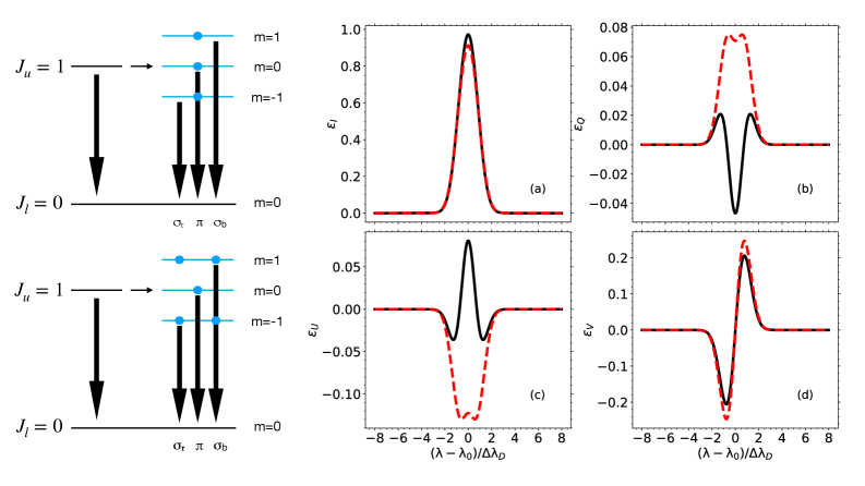
Figure 2: The two panels to the left illustrate the Zeeman splitting of the energy levels corresponding to a transition between atomic levels with $J_{u}=1$ and $J_{l}=0$. The top left panel shows the case of an evenly distributed population among the magnetic sublevels, while the bottom left panel shows an uneven distribution. The relative populations are indicated by the blue circles on the blue horizontal lines representing the magnetic sublevels. The quantization $\mathcal{Z}$–axis is taken along the magnetic field. The central and right columns show the calculated emission profiles for the Stokes $I$, $Q$, $U$, and $V$ parameters, respectively, assuming a Zeeman splitting of $\Delta\lambda_{D}/2$. The reference direction for positive Stokes $Q$ is defined by an azimuth $\chi$ with respect to the transverse component of the magnetic field. When $\chi=0$, i.e. when the reference direction is parallel to the transverse component of the magnetic field, the Stokes U signal vanishes. The black solid and red dotted curves correspond to the emissivity with evenly and unevenly distributed populations, respectively. The Stokes $I$ profile in the evenly distributed population case is normalized to its integral over wavelength. In the unevenly distributed population case, the relative intensities of the $\pi$ and $\sigma$ components are adjusted according to the population ratios shown in the bottom left panel (i.e., the ratio of populations for the the magnetic sublevels M = -1, 0, and 1 is 2:1:2).

The polarization that the Zeeman effect introduces in a spectral line is due to the wavelength shift of the transitions between the $M$ magnetic sublevels. In the Zeeman regime, this shift is given by [110],

$$\Delta\lambda=\Delta\lambda_{B}(g_{\ell}M_{\ell}-g_{u}M_{u})=4.6686\times 10^{-13}\lambda_{0}^{2}B(g_{\ell}M_{\ell}-g_{u}M_{u}),$$ (1)

where $\Delta\lambda$ is wavelength shift in Å, $\lambda_{0}$ is the central wavelength in Å of the unsplit transition, $B$ is magnetic field strength in gauss, $g_{u}$ and $g_{\ell}$ are the Landé factors of the upper and lower atomic levels, respectively, and $M_{u}$ and $M_{\ell}$ are the magnetic quantum numbers of the upper and lower magnetic sublevels, respectively. For dipole-type transitions, only those transitions with $\Delta M=M_{u}-M_{\ell}=0,\pm 1$ are permitted. The transition with $\Delta M=0$ is referred to as the $\pi$ component, and those with $\Delta M=\pm 1$ are the $\sigma_{b}$ and $\sigma_{r}$ components, respectively. The magnetic splitting of a given level is often characterized by the equation for a classical Zeeman triplet [e.g., 110, Sect. 3.3],

$$\Delta\lambda=\bar{g}\Delta\lambda_{B},$$ (2)

where $\bar{g}$ is the effective Landé factor.

The top left panel of Fig. 2 illustrates the Zeeman splitting of the energy levels corresponding to a transition from an upper level with $J_{u}=1$ to a lower level with $J_{l}=0$. The upper level splits into three magnetic sublevels, whereas the lower level remains unsplit because it has $J_{l}=0$. The resulting spectral line consists of $\pi$ and $\sigma$ components, each with a different polarization state. In the absence of a magnetic field, these components coincide in wavelength, and their polarization states cancel out, resulting in no net polarization (assuming an even population distribution among the magnetic sublevels). However, when a magnetic field is present, the energy splitting causes each component to have a different wavelength, preventing their polarization states from cancelling out and producing a net observable polarization.

The observed polarization depends on the relative direction between the magnetic field and the line-of-sight (LOS). For instance, the Zeeman induced polarization is purely circular when the LOS is parallel to the magnetic field, and purely linear when it is perpendicular. For any other viewing direction, the observed polarization is elliptical.

The emission coefficients for the Stokes parameters of an atom with Zeeman splitting are given by [e.g., 63],

$$\epsilon_{I} =C[\phi_{p}\sin^{2}\theta+\frac{\phi_{b}+\phi_{r}}{2}(1+\cos^{2}\theta)],$$ (3a)

$$\epsilon_{Q} =C(\phi_{p}-\frac{\phi_{b}+\phi_{r}}{2})\sin^{2}\theta\cos 2\chi,$$ (3b)

$$\epsilon_{U} =C(\phi_{p}-\frac{\phi_{b}+\phi_{r}}{2})\sin^{2}\theta\sin 2\chi,$$ (3c)

$$\epsilon_{V} =C(\phi_{r}-\phi_{b})\cos\theta,$$ (3d)

where $C$ is a constant which depends on the plasma properties. $\phi_{p,b,r}$ correspond to the emission profiles of the $\pi$, $\sigma_{b}$, and $\sigma_{r}$ components, respectively. $\theta$ is the inclination of the magnetic field with respect to the LOS, and $\chi$ is the azimuth of the transverse component of the magnetic field with respect to the positive Stokes $Q$ reference direction.

The black solid curves in the middle and right panels of Fig. 2 show the emission coefficients calculated corresponding to $\theta=\pi/3$ and $\chi=\pi/3$. Gaussian profiles with a Doppler width $\Delta\lambda_{D}$ were assumed for $\phi_{p}$, $\phi_{r}$, and $\phi_{b}$. The wavelength shifts of the $\sigma$ components were assumed to be $\Delta\lambda_{D}/2$. Additionally, the population was assumed to be evenly distributed among the magnetic sublevels.

Although in the chosen example the transverse magnetic field component is stronger than the longitudinal component, the resulting linear polarization is weaker than the circular polarization. This is because, in the weak field regime ($\Delta\lambda_{B}\ll\Delta\lambda_{D}$), the amplitude of the circular polarization induced by the Zeeman effect scales linearly with the ratio of the Zeeman splitting to the Doppler width, whereas the linear polarization scales with the square of this ratio [110]. Even if this argument is strictly correct only in the weak-field regime, the relation remains essentially valid for stronger fields. In the chromosphere, where the magnetic fields are typically weaker than in the photosphere and spectral lines tend to be wider, this ratio usually is much smaller than unity, making the detection of transverse magnetic fields especially challenging.

3.2 Atomic level polarization

The black solid curves in Fig. 2 were computed under the assumption that the atomic level populations are evenly distributed among magnetic sublevels. However, this assumption is not always suitable, especially in rarefied plasmas [181]. The population imbalance, illustrated in the bottom left panel of Fig. 2, modifies the relative intensities of the $\pi$ and $\sigma$ components, leading to a noticeable difference in the Stokes profiles of the emergent spectral line radiation. Even in the absence of a magnetic field, such population imbalance is capable of producing polarization, dubbed scattering polarization. In the solar atmosphere, the population imbalances arise from anisotropic optical pumping [50, 81], a process in which the absorption and scattering of anisotropic radiation leads to unequal populations among the magnetic sublevels. Furthermore, the population imbalances can occur among the magnetic sublevels of both the upper and lower levels [183, 180, 184, 121]. The magnetic sublevels can be not only unevenly populated, but they can also be quantum mechanically coupled [110]. The term atomic level polarization refers to both the population imbalance and to the quantum coherence among the magnetic sublevels of any given atomic level.

The scattering polarization signals are particularly significant near the solar limb. Spectropolarimetric observations throughout the solar spectrum from 3165 Å to 9950 Å at $\mu=0.1$ ($\mu=\cos\theta$, with $\theta$ the heliocentric angle) reveal a wealth of linearly polarized spectral structures [177, 178, 176], which was dubbed the Second Solar Spectrum by Ivanov [89]. An atlas of the Second Solar Spectrum, covering the wavelengths from the near UV to the near infrared, was subsequently obtained by Gandorfer [73, 74, 75], using the Zurich Imaging Polarimeter [ZIMPOL, 145, 146, 76].

The polarization of the atomic levels can be described using the irreducible spherical tensor components of the density matrix, $\rho^{K}_{Q}(\alpha J,\alpha^{\prime}J^{\prime})$ [69, 137], where $\alpha$ and $\alpha^{\prime}$ indicate the atomic states (i.e., electronic configuration). In most cases, quantum interference between the sublevels pertaining to different atomic levels (i.e., $\alpha J\neq\alpha^{\prime}J^{\prime}$) is negligible. The coherence between $J$-states pertaining to the same atomic term will be discussed in Section 3.4.

For $\alpha J=\alpha^{\prime}J^{\prime}$, the rank $K=0,1,\dots,2J$, and $Q=-K,-K+1,\dots,K$. The component $\rho^{0}_{0}(\alpha J)$ is proportional to the total population of the atomic level. The tensor components with $K=2$ are referred to as the alignment components and contribute to the linear polarization, while those with $K=1$ are referred to as the orientation components and contribute to the circular polarization. The components with $Q=0$ describe the distribution of the population among the magnetic sublevels, while those with $Q\neq 0$ describe the quantum coherence between magnetic sublevels and are generally complex numbers.

The density matrix tensor components with $K=1$ cannot usually be excited by unpolarized incident radiation, but they can be generated through alignment–orientation conversion in the presence of an electric field [35, 154], making them a potential means for the diagnostic such fields [9]. For atomic levels with $J\leqslant 1/2$, the maximum rank $K_{\rm max}\leqslant 1$, implying that no alignment components exist. Therefore, there cannot be linear scattering polarization in transitions between levels with $J\leqslant 1/2$, which is the case for the Mg II h line.

3.3 Hanle effect

The atomic level polarization can be modified by a magnetic field, which in turn leads to a modification of the line scattering polarization. This mechanism is dubbed Hanle effect after the discovery in the laboratory by Hanle (1924; see also Trujillo Bueno 181). This effect causes both a rotation and a change in the amplitude of the linear scattering polarization. The Hanle effect arises from the modification of the quantum coherence between the magnetic sublevels of an atomic state.

The modification of the atomic level polarization by a magnetic field due to the Hanle effect for a two-level atom (neglecting stimulated emission and assuming an unpolarized lower level) can be described by [110],

$$\rho^{K}_{Q}(J_{u})=\frac{1}{1+iQH_{u}}[\rho^{K}_{Q}(J_{u})]_{B=0},$$ (4)

where the quantization axis is taken parallel to the magnetic field vector. $\rho^{K}_{Q}(J_{u})$ are the irreducible spherical tensor components of the density matrix in the presence of a magnetic field, while the subscript $B=0$ denotes the field-free case. The dimensionless Hanle parameter, $H_{u}$, is defined as $H_{u}=0.879\times 10^{7}t_{\rm life}gB$, where $t_{\rm life}$ is the lifetime (in seconds) of the atomic level under consideration, $g$ is its Landé factor, and $B$ is the magnetic field strength (in gauss).

From Eq. (4), the Hanle effect does not operate when the magnetic field is too weak ($H_{u}\ll 1$), and it saturates for sufficiently strong magnetic fields ($H_{u}\gg 1$), in which case the quantum coherence terms with $Q\neq 0$ vanish. The Hanle effect is thus sensitive to magnetic field strengths within an approximate range of $0.2B_{\rm H}<B<5B_{\rm H}$, where $B_{\rm H}$ is the critical Hanle field given by [e.g., 182],

$$B_{\rm H}=\frac{1.137\times 10^{-7}}{t_{\rm life}g}.$$ (5)

The critical magnetic field of the Mg II k line is listed in Table 1, with $t_{\rm life}$ being roughly estimated as $A_{ul}^{-1}$. Hence, the Hanle effect of the Mg II k line is roughly sensitive to magnetic field strengths between 4 G and 110 G, approximately. In contrast to the Zeeman effect, the Hanle effect is sensitive to tangled magnetic fields at subresolution scales [174]. This has enabled the detection of a substantial amount of hidden magnetic energy in the quiet Sun [185].

3.4 $J$-state interference

As mentioned in Section 3.2, the density matrix components $\rho^{K}_{Q}(\alpha J,\alpha^{\prime}J^{\prime})$ with $\alpha J\neq\alpha^{\prime}J^{\prime}$, which describe the quantum interference between $J$-states, are usually neglected. However, within a given atomic term ($\alpha=\alpha^{\prime}$), when the energy separation between the levels $\alpha J$ and $\alpha J^{\prime}$ is sufficiently small, these components can become significant. In particular, when PRD effects are important, $J$-state interference can have a substantial impact on the spectral line polarization. This is the case for spectral lines such as the Ca II H and K lines, the Mg II h and k lines, and the Na I $\rm D_{1}$ and $\rm D_{2}$ lines [16, 173, 19]. Generally, $J$-state quantum interference leads to polarization features in the wings of spectral lines [18].

The impact of quantum interference between the upper levels of the Mg II h and k lines in the absence of a magnetic field was first predicted by [16], who assumed coherent scattering in the observer’s frame, an approximation reasonable only in the far wings. Their modeling predicted that the Stokes $Q$ profile exhibits strong positive polarization signals toward the red wing of the h line and toward the blue wing of the k line, while becoming negative in the spectral region between the two lines. This prediction was later confirmed by Belluzzi and Trujillo Bueno [19], considering $J$-state interference and PRD effects, and by del Pino Alemán et al. [60, 61] and Alsina Ballester et al. [7], including arbitrary magnetic fields.

The Ultraviolet Spectrometer and Polarimeter [UVSP, 208] aboard the Solar Maximum Mission [24] acquired observations of the linear polarization across the Mg II h and k lines. While the first analysis by [82] did not reveal significant linear polarization in the spectral region of the wings between these two lines, a subsequent reanalysis by Manso Sainz et al. [124] detected negative Stokes $Q$ polarization. This finding was clearly confirmed by the high-precision spectropolarimetric observations acquired by the CLASP2 sounding rocket experiment [149]. These unprecedented observations also confirmed the theoretical prediction of Belluzzi and Trujillo Bueno [19] for the whole spectral range of the Mg II h and k lines, including the near wings around the centers of these lines.

3.5 Magneto-optical effects

The significant scattering polarization Stokes $Q$ signals in the line wings of the Mg II h and k lines can give rise to significant Stokes $U$ signals through the M-O effects in the presence of a longitudinal magnetic field. The radiative transfer (RT) equations for Stokes $Q$ and $U$ are given by,

$$\frac{dQ}{ds} =\epsilon_{Q}-\eta_{Q}I-\rho_{V}U+\rho_{U}V-\eta_{I}Q\simeq\epsilon_{Q}-\rho_{V}U-\eta_{I}Q,$$ (6a)

$$\frac{dU}{ds} =\epsilon_{U}-\eta_{U}I+\rho_{V}Q-\rho_{Q}V-\eta_{I}U\simeq\epsilon_{U}+\rho_{V}Q-\eta_{I}U,$$ (6b)

where $\epsilon_{I,Q,U,V}$ and $\eta_{I,Q,U,V}$ are the emission and absorption coefficients for the four Stokes parameters, respectively. The $\rho_{Q,U,V}$ terms are responsible for the M-O effect. For the Mg II h and k lines, $\rho_{V}$ is negligible at the line center, but becomes significant in the line wings, as its spectral shape results from the superposition of antisymmetric dispersion profiles [see 5]. Consequently, the terms $\rho_{V}U$ and $\rho_{V}Q$ lead to a rotation of the linear polarization introducing sensitivity in the line wings of Stokes $Q$ and $U$ to the presence of magnetic fields as weak as those that activate the Hanle effect at the center of the k line [see 5]. The manifestation of the M-O effects discussed here requires a significant scattering polarization signal in the wings of the spectral lines. Therefore, these M-O effects are intimately associated with the $J$-state interference and PRD effects, which is why we often distinguish them from the well-known M-O effect caused by the Zeeman effect in the presence of strong magnetic fields [110], which is significant in the line core region without the need of scattering polarization.

3.6 Partial frequency redistribution

A rigorous quantum physics framework for describing the Hanle effect was built by Landi Degl’Innocenti and Landi Degl’Innocenti [107], Bommier and Sahal-Brechot [29], Bommier [25], and Landi Degl’Innocenti [103, 104, 105, 106] under the assumption of complete frequency redistribution (CRD). The CRD assumption is valid in highly collisional plasmas, where collisions destroy the coherence between the incident and the emitted radiations, or when this coherence is negligible because the incident radiation is spectrally-flat across the spectral line under consideration, also known as the flat-spectrum approximation [37]. In both cases the scattering processes can be treated as a temporal succession of statistically independent first-order processes. Sahal-Brechot [158, 157, 159], and Casini and Judge [36] extended the formalism from electric to magnetic dipole transitions. More recently, Casini et al. [43] extended it to electric and magnetic quadrupolar transitions. In this quantum mechanical theoretical framework, the statistical equilibrium (SE) equations governing the density matrix, and the RT equations for the Stokes parameters are derived self-consistently from the theory of quantum electrodynamics.

For strong resonance lines such as the Mg II h and k lines, the Ca II H and K lines, or the H I Ly-$\alpha$ line, the coherence between the absorbed and the emitted photons is not negligible. This coherence leads to a dependence of the emission profile on both the incoming and outcoming frequencies of the photon [84, 131], which is referred to as PRD. The effects of PRD have been taken into account in forward modeling and inversion codes in one dimensional (1D) plane parallel atmospheric models, such as RH [192, 142], STiC [55, 56], and HanleRT-TIC [60, 114], with the latter accounting for the joint action of the Zeeman and Hanle effects, and scattering polarization. PRD effects have also been accounted for in three dimensional (3D) non-LTE RT calculations by Sukhorukov and Leenaarts [179], albeit without polarization. Accounting simultaneously for PRD effects, atomic level polarization, the Hanle and Zeeman effects, in 3D non-LTE RT calculations remains a significant challenge. However, promising progress has been made in this regard [e.g., 23].

By extending the impact theory of pressure broadening [10, 17, 70], the frequency redistribution function for a polarized atomic system was derived by Omont et al. [138, 139] and Domke and Hubeny [66]. Bommier [26, 27] advanced the theoretical framework mentioned in Section 3.3 by including higher-order terms in the perturbative expansion of the atom-radiation interaction, under the assumption of a two-level atom model with an unpolarized and infinitely sharp lower level. Later, quantum interference between $J$-states within the same atom term was incorporated into the frequency redistribution function for a two-term atom [167, 168, 28]. Independently, using a different theoretical approach, Casini et al. [39], Casini and Manso Sainz [38], and Casini et al. [40, 41] derived the frequency redistribution function and corresponding expression for the emissivity for $\Lambda$-type atomic systems. Applying the quantum theories proposed by Bommier [26, 27, 28] and Casini et al. [39], Alsina Ballester et al. [5, 7] and del Pino Alemán et al. [60, 61] independently developed 1D RT codes capable of accounting for the Hanle and Zeeman effects, PRD effects, as well as atomic polarization and $J$-state interference. Recently, [153] demonstrated that both approaches yield identical polarization profiles for the Mg II h and k lines when modeled with a two-term atomic model.

To reduce computational cost, the angle-average approximation is commonly employed when solving the RT problem with PRD effects. This approach decouples the angular and frequency dependencies of the redistribution functions by averaging the redistribution matrix over all directions [131, 111, 20, 6], thereby significantly accelerating the calculation compared with the general angle-dependent treatment. For the polarized case, the averaging of the redistribution matrix is performed excluding the scattering phase matrix [151]. However, it is important to note that the this approximation can significantly impact the resulting polarization for some spectral lines, often around the line cores in the linear polarization profiles [135, 163, 90, 78, 22].

For specific spectral lines, the angle-average treatment of PRD effects remains a valid approximation. For instance, Riva et al. [152] demonstrated that this approximation provides reliable modeling of the Stokes profiles of the He II Ly-$\rm\alpha$ at 30.4 nm. del Pino Alemán et al. [62] showed, using a 1D semi-empirical atmospheric model with magnetic fields, that angle-dependent effects can lead to measurable differences in the linear polarization near the core of the Mg II k line. Nonetheless, these authors pointed out that the impact of the angle-averaged approximation in the Mg II k line is considerably reduced at the spectral resolution and polarimetric accuracy of the CLASP2 observations.

4 Forward modeling of the Mg II h and k line polarization

The broad polarization pattern in the far wings of the Mg II h and k lines was first pointed out by Auer et al. [16], who performed a simplified RT calculation by assuming fully coherent scattering in the observer’s frame, which is a reasonable approximation for the far wings of spectral lines. A more rigorous radiative transfer investigation of the linear polarization across the entire Mg II h and k linear polarization, in the absence of magnetic fields, was later carried out by Belluzzi and Trujillo Bueno [19], using a two-term atomic model. Their results predicted an antisymmetric shape of the $Q/I$ profile around the center of the h line, and two negative troughs to the sides of a positive $Q/I$ peak at the center of the k line. These theoretical predictions were subsequently confirmed by the high-precision spectropolarimetric observation acquired by the CLASP2 sounding rocket experiment [see 149].

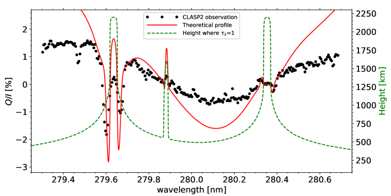
Figure 3: Temporally and spatially averaged $Q/I$ profile at $\mu=0.1$ observed by CLASP2 (black dots), $Q/I$ profile resulting from the forward synthesis in the FAL-C semi-empirical model with a three-term Mg II atomic model in the absence of a magnetic field (red curve), and height where the optical depth at each wavelength is unity for $\mu=0.1$ (green dashed curve), corresponding to the scales on the right axis. The reference direction for positive Stokes $Q$ is the parallel to the nearest solar limb. The CLASP2 observational data are reproduced with permission from Rachmeler et al. [149].

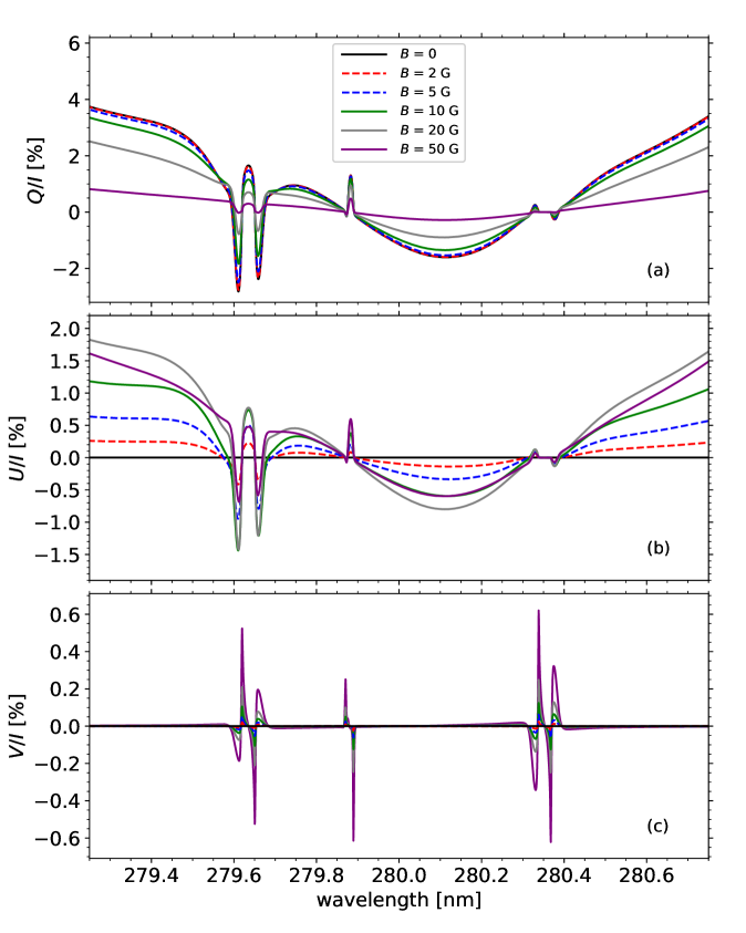
Figure 4: Synthetic $Q/I$ (panel a), $U/I$ (panel b), and $V/I$ (panel c) Mg II h and k profiles in the FAL-C semi-empirical model for a LOS with $\mu=0.1$. The different color curves correspond to calculations with magnetic fields inclined 45^∘ with respect to the local vertical toward the observer, with different strengths indicated by the color (see legend in panel a). The asymmetry in the $V/I$ profile at 279.88 nm arises because it actually consists of two blended spectral components. This figure is similiar to that in del Pino Alemán et al. [61], but with a magnetic field with a different direction and strength.

The black dots in Fig. 3 show the temporally and spatially averaged $Q/I$ profiles observed by CLASP2 near the solar limb. Both the Mg II h and k lines, as well as the subordinate lines at 279.88 nm were observed. The red curve shows the forward synthesis with HanleRT-TIC in the C model of Fontenla et al. [71, here after FAL-C model] using a three-term atomic model including five levels of Mg II and the ground level of Mg III (see also Figure 7 of Trujillo Bueno and del Pino Alemán 182). The green dashed curve indicates the height where the optical depth at each wavelength equals unity, providing a rough estimate of the formation heights.

The observed $Q/I$ profile shows a positive signal at the center of the Mg II k line, with negative troughs on either side. As expected, the center of the Mg II h line exhibits no $Q/I$ signal, because both the upper and lower levels have total angular momentum $J=1/2$ and thus cannot carry atomic alignment. Consistent with theoretical predictions [see 19], the antisymmetric $Q/I$ signal around the center of the h line, caused by PRD effects and $J$-state interference, was also detected by CLASP2. The polarization signals in the far wings, particularly the negative $Q/I$ signal in the region between the h and k lines, are clearly confirmed as well.

Although the synthesized profiles in Fig. 3 reproduce the overall shape of the observed linear polarization, there are clear differences in both the width and amplitude of the profile. Part of these differences are due to the instrument’s point spread function (PSF), which is not considered in the theoretical profiles, as well as to that the FAL-C model is an idealization of the real solar atmosphere. Nevertheless, the main reason for the difference in the amplitude of the $Q/I$ signals is that this calculation was performed without including magnetic fields. The presence of a magnetic field leads to depolarization of the $Q/I$ profiles, as illustrated in panel (a) of Fig. 4. The amplitude variation of the polarization demonstrates their valuable diagnostic potential for inferring the magnetic field properties of the chromospheric plasma.

The magnetic sensitivity of the Mg II h and k lines has been studied using a two-level atomic model focusing only on the k line [5], a two-term atomic model [60, 123], and a three-term atomic model including the subordinate lines [61]. Figure 4 illustrates the Stokes profiles of the Mg II h and k lines, as well as the subordinate lines, synthesized in the FAL-C semi-empirical model for a LOS with $\mu=0.1$. The magnetic fields are inclined by 45^∘ toward the observer with respect to the local vertical, with strengths ranging from 0 to 50 gauss. The impact on the linear polarization at the center of the k line is dominated by the Hanle effect, which also operates on the subordinate lines. In the wings, the magnetic sensitivity of the linear polarization signals arises from M-O effects. The Stokes $V$ profiles of the h and k lines, primarily caused by the Zeeman effect, exhibit four lobes. The inner lobes originate in the upper chromosphere, while the outer lobes originate at relatively lower chromospheric heights.

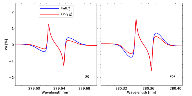
Figure 5: $V/I$ profiles of the Mg II k (panel a) and h (panel b) lines in the FAL-C semi-empirical model for a LOS with $\mu=1.0$ and for a magnetic field of 100 G parallel to the LOS. The blue (red) curves correspond to the calculation including (neglecting) scattering polarization. This figure is similar to that in Alsina Ballester et al. [5].

The outer lobes of the circular polarization are also impacted by the joint action of PRD effects and the radiation field anisotropy [5, 60]. Figure 5 shows that accounting for the radiation field anisotropy results in an enhancement of the signal of the outer lobes of the Stokes $V$ profiles. This enhancement is present even in the Mg II h line, despite the fact that its levels cannot carry atomic alignment. If the radiation field anisotropy and the atomic polarization are neglected in an inversion, these enhanced outer lobes will lead to an overestimation of the inferred longitudinal magnetic field [114].

5 Non-LTE Stokes inversion

Inversion techniques are our most powerful tools to extract the physical information encoded in spectral lines [64, 150]. The most advanced inversion codes can retrieve the stratification of magnetic field, temperature, electron density, gas pressure, and LOS and microturbulent velocities from spectropolarimetric observations, usually under the assumption of hydrostatic equilibrium.

The SIR code [155] was the first inversion tool capable of recovering a stratified model atmosphere from spectropolarimetric observations. Although SIR assumes LTE and is thus restricted to photospheric lines, it made use of several important concepts, such as nodes, RFs, and the assumption of hydrostatic equilibrium to retrieve a stratification of the gas pressure. These concepts have been adopted in subsequent depth-stratified inversion codes, such as SPINOR [72], NICOLE [169, 170], SNAPI [133], STiC [55, 56], DeSIRe [156], FIRTEZ [141, 30], or HanleRT-TIC [60, 61, 114].

Inversion codes usually start with the synthesis of the line profiles from an initial guess of the atmospheric model. This model is parameterized using a prescribed number of nodes, from which a fine stratification of the atmospheric parameters is interpolated. Iterative corrections to the model parameters at these nodes, based on RFs, are applied until the best fit to the observations is achieved. Typically, the Levenber-Marquardt algorithm [147] is employed to minimize a cost function. Given that the inversion problem is inherently ill-posed, and there are often degeneracies between model parameters, regularization terms are usually included in the cost function. The regularization terms favor smooth stratifications of the model parameters over complex ones by employing penalties on these model parameters.

The RFs describe the response (or change) of any given Stokes parameter of the emergent radiation at any given wavelength to a perturbation of one of the model parameters at a specific location in the model atmosphere. In some inversion codes, they can be computed analytically or semi-analytically, as in SIR, SNAPI, FIRTEZ, and DeSIRe, while in others they are calculated numerically, as in NICOLE, STiC, and HanleRT-TIC. In the numerical approach, the RFs are obtained by perturbing the value at a single node and synthesizing the Stokes profiles in the resulting model atmosphere. This method is computationally expensive because it requires multiple spectral syntheses to obtain the RFs. Therefore, inversion codes following an analytical approach for the calculation of the RFs are usually faster than their numerical counterparts. However, their efficiency and accuracy have only been validated in the absence of atomic level polarization [132]. Moreover, deriving analytical RFs requires an explicit treatment of all interdependencies in the SE equations, which becomes significantly challenging when including PRD effects or atomic polarization.

With the exception of HanleRT-TIC, all the above-mentioned inversion codes only take into account the Zeeman effect as polarization mechanism, and cannot handle most of the physical mechanisms discussed in Section 3. A well-known exception not yet mentioned is the HAZEL code [13], which includes atomic level polarization as well as the Zeeman and Hanle effects, albeit under the assumption of an optically thin and homogeneous slab model. HAZEL is commonly used for inverting spectropolarimetric observations of the He I triplet at around 1083.0 nm and the He I D₃ lines [e.g. 140, 128, 68]. Although HAZEL is mainly applied to prominence and filament observations, it has also been applied to other regions such as plages [8] and spicules [44, 126]. Nevertheless, the HAZEL code is not suitable for other chromospheric lines formed in optically thick plasmas, such as the Mg II h and k lines. Moreover, it does not account for PRD effects.

To infer the magnetic field vector from spectropolarimetric observations of the Mg II h and k lines, Li et al. [114] developed the Tenerife Inversion Code (TIC), which employs the HanleRT synthesis code [60, 61] as its forward modeling engine. HanleRT (the forward modeling module) and TIC (the Stokes inversion module) are now referred to as the HanleRT-TIC radiative transfer code. HanleRT-TIC is a 1D non-LTE spectral synthesis and inversion code capable of accounting for all the physical mechanisms introduced in Section 3, which are critical for modeling the polarization of the Mg II h and k lines. To solve the system of linear equations for obtaining the corrections to the model parameters from the numerically calculated Hessian matrix, the code uses the modified singular value decomposition (SVD) method used by [155]. Moreover, electron and hydrogen number densities are computed under the assumption of LTE by solving the equation of state using the method of Wittmann [207], as implemented in the SIR code.

The uncertainties of the model parameters at each node are estimated following the approach described in Sánchez Almeida [164] and del Toro Iniesta [63],

$$\sigma_{p}^{2}=\frac{\Delta\chi^{2}}{2N}H^{-1},$$ (7)

where $N$ is the number of nodes, $\Delta\chi^{2}$ is the cost function excluding the regularization term, and $H^{-1}$ is the inverse of the Hessian matrix. In practice, $H^{-1}$ is often approximated by the inverse of the diagonal elements of the Hessian matrix. Since these diagonal elements are, in fact, the squares of the RFs, the uncertainties can be estimated directly from the RFs themselves. Although this method does not provide precise uncertainty estimates, it provides a relative indication of how well each model parameter is constrained at a given node.

A more robust approach to estimate the uncertainties of the model parameters is the Monte Carlo approach [205, 160, 117]. In this method, a number of different Stokes profiles are generated by adding random noise consistent with the observational uncertainties to the measured profiles. The inversion of all these profiles produces a statistical distribution of inferred model parameters, which in turn provides a more accurate representation of the uncertainties.

6 Weak-field approximation

In addition to non-LTE inversions, the WFA is often employed for a rapid estimation of the magnetic field from the Stokes profiles. The WFA is applicable when the Zeeman splitting is much smaller than the Doppler width. The WFA expressions were derived by Landi Degl’Innocenti and Landi Degl’Innocenti [108] using perturbation theory, and by Jefferies et al. [92] via Taylor series expansion. These equations are given by [see 110],

$$V(\lambda) =-\Delta\lambda_{B}\bar{g}\cos\theta\left(\frac{\partial I}{\partial\lambda}\right).$$ (8a)

$$\tilde{Q}(\lambda_{0}) =-\frac{1}{4}\Delta\lambda^{2}_{B}\bar{G}\sin^{2}\theta\left(\frac{\partial^{2}I}{\partial\lambda^{2}}\right)_{\lambda_{0}}.$$ (8b)

$$\tilde{Q}(\lambda_{\rm w}) =\frac{3}{4}\Delta\lambda^{2}_{B}\bar{G}\sin^{2}\theta\frac{1}{\lambda_{\rm w}-\lambda_{0}}\left(\frac{\partial I}{\partial\lambda}\right)_{\lambda_{\rm w}}.$$ (8c)

$$\frac{U(\lambda)}{Q(\lambda)} =\tan 2\chi.$$ (8d)

where $\tilde{Q}$ indicates the Stokes $Q$ parameter in the reference system where Stokes $U$ is zero, and $\bar{G}$ is a constant that depends on the quantum numbers of the levels involved in the transition. Eq. (8a) can be used to estimate the longitudinal component of the magnetic field. Eqs. (8b) and (8c) can be used to estimate the transverse component, and they are valid in wavelengths close to the line center ($\lambda_{0}$) and in the line wings ($\lambda_{\rm w}$), respectively. Finally, the azimuth of the magnetic field can be inferred from Eq. (8d).

Although the WFA assumes height-independent physical parameters in the formation regions of the spectral lines and neglects atomic polarization and PRD effects, it enables a very fast estimation of the magnetic field. Note that Eq. (8a), the WFA for Stokes $V$, only requires that the longitudinal component of the magnetic field is constant in the formation region. The WFA has been successfully applied in numerous studies to extract the magnetic field vector from spectropolarimetric observations, [e.g., 125, 127, 134, 67, 165, 148].

The reliability of the WFA for estimating the longitudinal magnetic field from the Mg II h and k lines has been studied by del Pino Alemán et al. [60], Centeno et al. [46], and Afonso Delgado et al. [1]. From spectropolarimetric syntheses performed in the FAL-C atmospheric model, Centeno et al. [46] found that applying the WFA to all four lobes of the Stokes $V$ profile results in an underestimation of the longitudinal magnetic field by approximately 13%, whereas the values derived from only the inner lobes closely match the input magnetic field strength. Furthermore, spectral degradation to a resolution of 30 000, similar to that of CLASP2, increases the error to approximately 18% and 10% when derived from the four lobes and inner lobes, respectively.

7 Interpretation of the Observations

The intensity profiles of the Mg II h and k lines have been routinely observed by the IRIS satellite since 2014, with a spectral sampling of 25.4 mÅ pixel^-1. The non-LTE inversion of the intensity profiles of the Mg II h and k lines can be performed using, for example, the STiC code, which is built upon the RH code [192], and is thus capable of accounting for PRD effects and the Zeeman effect. Lately, Sainz Dalda et al. [161, 162] built a database, dubbed IRIS², which contains representative intensity profiles of the Mg II h and k lines observed by IRIS. The corresponding representative atmospheric models were obtained using the STiC inversion code. By matching observed profiles to this precomputed database, IRIS² enables a very quick estimation of the inferred model atmosphere, with a reduction of computational cost of about 10⁵ - 10⁶, while maintaining an accuracy comparable to that of the full inversion.

The Mg II h and k lines provide constraints on the chromospheric temperature and turbulent velocity [196, 32]. da Silva Santos et al. [52] performed an inversion of IRIS observations of the Mg II h and k lines together with radio observations at 1.25 mm from the Atacama Large Millimeter/submillimeter Array [ALMA, 209] using the STiC code. Their results placed robust constraints on the temperature and turbulent velocity over a wide range of heights. Additionally, an inversion based on the IRIS² database, carried out by Bose et al. [31], revealed a strong correlation between the heating in plage and moss regions. These studies demonstrate the diagnostic potential of the Mg II h and k lines for probing the thermodynamic properties in the chromosphere. For a comprehensive overview of the results achieved by IRIS, see De Pontieu et al. [59].

7.1 CLASP2 and CLASP2.1 observations

In order to demonstrate the theoretically predicted diagnostic potential of the Mg II h and k lines for studying chromospheric magnetic fields, the CLASP2 sounding rocket was launched on April 11, 2019, measuring the Stokes profiles of these lines. The observed spectral range spanned from 279.30 to 280.68 nm, covering the Mg II h and k lines, the subordinate lines at 279.88 nm, and the Mn I lines at 279.91 and 280.19 nm with a spectral sampling of 49.9 mÅ pixel^-1. The full width at half-maximum (FWHM) of the instrument’s profile, resulting from the convolution of the slit width with the spectral PSF, is 110 mÅ [171, 190].

During the $\sim$5 min observation window, CLASP2 performed sit-and-stare observations using a 196” long spectrograph slit positioned at an active-region plage and a quiet Sun region close to the limb. The spatial resolution along the slit direction was 0.53” per pixel, and the polarization accuracy was better than 0.1%.

Motivated by the success of this suborbital mission, a reflight of CLASP2, dubbed CLASP2.1, was carried out on October 8, 2021. Instead of the sit-and-stare observation, CLASP2.1 scanned a two-dimensional field of view over an active region plage located near a sunspot with a raster step size of approximately 1.8”. CLASP2.1 measured the full Stokes parameters in the same spectral range as CLASP2. However, the polarimetric accuracy was slightly worse (around $10^{-3}$ at the intensity peaks of the Mg II h and k lines), due to the reduced integration time. For further details on the CLASP2 and CLASP2.1 missions and their observations, see Ishikawa et al. [86, 87], Rachmeler et al. [149], Trujillo Bueno and del Pino Alemán [182], Li et al. [117], Song et al. [172], Ishikawa et al. [88] and Afonso Delgado et al. [4].

7.2 Inversion of the Stokes $I$ and $V$ profiles

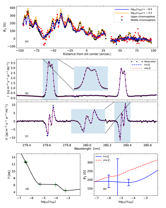
Figure 6: Longitudinal magnetic field inferred from the application of the WFA to the inner (red dots) and outer (black dots) lobes of the $V/I$ profiles of the Mg II h and k lines obtained by CLASP2 [86]. Longitudinal magnetic field inferred from the inversion of the intensity and circular polarization profiles of the Mg II h and k lines at log${}_{10}(\tau_{500})=-6.0$ (blue curve in panel a) and $-4.5$ (orange curve in panel a) from Li et al. [115]. Panels (b) and (c) show the observed (black dots) and fit (dashed blue and dotted red curves) Stokes $I$ and $V$ profiles for a pixel in the plage region. The dashed blue (dotted red) curves in panels (b) and (c) correspond to the inversion including (neglecting) the anisotropy terms. Panels (d) and (e) show the inferred temperature (black curve) and longitudinal component of the magnetic field from the inversion including (solid blue curve) and neglecting (dashed red curve) the anisotropy terms, for the same pixel, with error bars for the temperature and the magnetic field calculated including the anisotropy terms. The green “+” in panel (d) signal the position of the temperature nodes. Image reproduced with permission from Li et al. [115].

Given the complexity associated with interpreting the linear polarization of the Mg II h and k lines (see Section 3), Ishikawa et al. [86] first analyzed the Stokes $I$ and $V$ profiles using the WFA. By applying the WFA independently to the inner lobes of the Mg II h and k lines, and to the outer lobes of the h line, they derived the longitudinal components of the magnetic fields in the upper (red circles in panel (a) of Fig. 6) and middle (black circles) chromosphere, respectively. Inside the magnetic flux concentrations, the inferred field strength reached up to 300 G in the middle and upper chromosphere. This value is consistent with the magnetic field strength reported by da Silva Santos et al. [53], and is slightly lower than those in Morosin et al. [134], which are inferred from the Ca II 854.2 nm by using the WFA. This discrepancy can be explained by that the observations were obtained from different target regions with different LOS directions, and that the Ca II 854.2 nm line is sensitive to relatively lower atmospheric layers than the Mg II h and k lines [51].

The same dataset was later analyzed by Li et al. [115] using HanleRT-TIC. Since the circular polarization is not impacted by $J$-state interference, it was neglected in the inversion to reduce the computational cost. The resulting longitudinal magnetic field at log${}_{10}(\tau_{500})=-6.0$ and $-4.5$, shown as the blue and orange curves in panel (a) of Fig. 6, respectively, closely match the results obtained using the WFA. An example of the inversion of the Stoke $I$ and $V$ profiles in the plage region is shown in panel (b) and (c), where the blue and red curves correspond to the fits from the inversions with and without the anisotropy terms, respectively. The temperature and the longitudinal magnetic field that resulted from the inversion are shown in panel (d) and (e), respectively. As seen in the figure, both inversion setups reproduce the observations well. As expected, the inversion without anisotropy terms required a stronger magnetic field in order to fit the circular polarization in the line wings, as discussed in Section 4. Although the impact of the anisotropy is expected to appear only in the outer lobes, primarily affecting the inference of the longitudinal magnetic field in the middle chromosphere, the spectral PSF couples different wavelengths, resulting in an impact also on the inferred magnetic field in the upper chromosphere.

The longitudinal magnetic field inferred from the WFA exhibits a strong correlation with the electron pressure (the product of temperature and electron density) derived from the IRIS² database [161], suggesting a magnetic origin of the chromospheric heating in active region plages [86]. This correlation was further confirmed by the non-LTE inversion results [115]. However, a similarly significant correlation is not observed in the results obtained from the inversion of the He I triplet at 1083.0 nm lines [8].

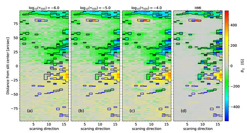
Figure 7: Panels (a), (b), and (c) display the longitudinal magnetic field at log${}_{10}(\tau_{500})=-6.0$, $-5.0$, and $-4.0$, respectively, resulting form the inversion of the CLASP2.1 observations. Panel (d) shows the corresponding HMI magnetogram. Blue and black contours indicate the HMI magnetic field strengths of 70 G and -70 G, respectively. Image reproduced with permission from Li et al. [117].

The CLASP2.1 mission enabled spatial scanning to capture a two-dimensional field of view of an active region plage located near a sunspot. Panels (a), (b), and (c) of Fig. 7 show the longitudinal magnetic fields at log${}_{10}(\tau_{500})=-6.0$, $-5.0$, and $-4.0$, respectively, obtained through pixel-by-pixel inversion of the Stokes $I$ and $V$ profiles [117]. The polarity of the magnetic field flux concentrations in the chromosphere is generally consistent with those found in the photosphere, as seen in the HMI magnetogram shown in panel (d). These magnetic field flux concentrations expand with height due to the lower gas pressure in the chromosphere compared to the photosphere, and thus occupy larger areas in the chromosphere.

The magnetic field obtained from the Stokes inversion shows strong correlation with the temperature and electron density in the chromospheric plage, as well as with the intensity of the AIA 171 Å band in the overlying moss region [117]. The correlation between the intensities of spectral lines formed in the moss region and in the underlying chromospheric plage have been reported by Vourlidas et al. [197], De Pontieu et al. [57], and Bose et al. [31], suggesting a possiblly common heating mechanism operating in both the chromospheric plage and the transition region moss. However, Judge et al. [96] reported an absence of such a correlation between the AIA 171 Å intensity and the chromospheric magnetic field inferred from the Ca II 854.2 nm line using WFA in a plage region that includes the footpoints of coronal loops, even though the heating appears to be concentrated around unipolar chromospheric magnetic field regions.

Overall, the polarities of the longitudinal magnetic fields in the upper and middle chromosphere obtained by CLASP2.1 are consistent. However, in certain regions, polarity changes with height have been reported by Li et al. [117] and Ishikawa et al. [88]. To verify the reliability of the polarity change, a Monte Carlo simulation was employed by Li et al. [117], confirming that the inferred field strengths exceed the uncertainties caused by the noise. Song et al. [172] reported a coronal loop brightening in the vicinity of the polarity change region, suggesting a possible connection between magnetic field geometry and coronal activity. Similar polarity reversals between the photosphere and chromosphere have also been reported by Mathur et al. [129] based on spectropolarimetric observations of photospheric and chromospheric lines. Even in the photosphere, polarity reversals can also been detected with the Fe I 630.1 and 630.2 nm lines [120].

7.3 Full Stokes inversion

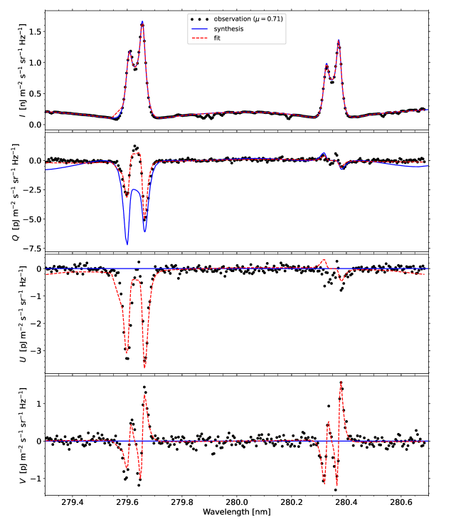
Figure 8: From top to bottom, Stokes $I$, $Q$, $U$, and $V$, respectively, of the Mg II k and h lines in a pixel of the plage region with $\mu=0.71$ acquired by CLASP2 (black dots). The blue curves correspond to synthetic Stokes profiles calculated in the non-magnetized model atmosphere resulting from the inversion of the intensity profile. The red curves show the full Stokes inversion results, including the parameterization of the radiation field tensor components ${J^{\dagger}}^{K}_{Q}$ and the magnetic field. Note that the $k_{1v}$ minimum is blended with a Mn I line at around 279.57 nm; thus the affected wavelength points were excluded from the inversion and from the plot, the reason why there is a straight line in that spectral region for the intensity. Image reproduced with permission from Li et al. [116].

In 1D atmospheric models without horizontal macroscopic velocities, the linear polarization can only be either parallel or perpendicular to the nearest solar limb, unless there is an inclined magnetic field. Under such circumstances, when either of these directions is chosen as the reference for linear polarization, Stokes $U$ can only arise in the presence of a magnetic field. However, in the real solar atmosphere, horizontal inhomogeneities in the plasma temperature and density, as well as the gradients of the horizontal components of the macroscopic velocity, are able to break the axial symmetry. As a result, Stokes $U$ can appear even in the absence of a magnetic field [122, 199, 91].

The black dots in Fig. 8 display the Stokes profiles observed by CLASP2 in a pixel within the plage region. The blue curves represent the Stokes profiles synthesized in the 1D non-magnetized model atmosphere obtained by inverting the intensity profile. As expected, the blue curves show zero signals in Stokes $U$ and $V$, while there is a clear Stokes $Q$ signal due to scattering polarization. Notably, the amplitude of the right trough of the k line in this synthetic Stokes $Q$ profile closely matches that of the observation. Given that the Hanle and M-O effects typically depolarize and rotate the linear polarization (transforming Stokes $Q$ into $U$ in this case), it is thus not possible to find a magnetic field vector that simultaneously reproduces all the observed Stokes $Q$, $U$, and $V$ profiles. This highlights the limitations of a 1D plane-parallel modeling and suggests that horizontal RT plays a significant role.

7.3.1 Parameterization of the lack of axial symmetry

In addition to the physical mechanisms mentioned in Section 3, axial-symmetry breaking caused by horizontal inhomogeneities and RT, i.e. 3D effects, must be taken into account when inverting the full Stokes profiles of the Mg II h and k lines. However, the development of such an inversion code that simultaneously accounts for PRD effects and $J$-state interference in full 3D remains a significant challenge.

In a 1D RT calculation, the model atmosphere is assumed to be plane-parallel, with axially symmetric plasma thermodynamic properties. As a result, in a non-magnetic and static 1D model the radiation field tensor components $J^{2}_{Q}$ with $Q\neq 0$ vanish [for a detailed description of the $J^{K}_{Q}$ tensor, refer to 110]. However, in a 3D atmosphere, where horizontal RT is taken into account, these components may be non-zero even in the non-magnetic and static case. There is thus a missing contribution to these tensor components in a 1D model atmosphere, which can lead to significant inaccuracies in the inversion of the linear polarization of the Mg II h and k lines.

Li et al. [116] proposed a method to parameterize this missing contribution and implemented it in the HanleRT-TIC code by introducing ad-hoc radiation field tensor components. Specifically, they define the radiation field tensor components as,

$$J^{\prime 2}_{1} =J^{2}_{1}+{J^{\dagger}}^{2}_{1},$$ (9a)

$$J^{\prime 2}_{2} =J^{2}_{2}+{J^{\dagger}}^{2}_{2},$$ (9b)

where $J^{2}_{1}$ and $J^{2}_{2}$ are the tensor components obtained from standard 1D RT calculations. ${J^{\dagger}}^{2}_{1}$ and ${J^{\dagger}}^{2}_{2}$ are the ad-hoc parameters that mimic the missing contributions due to 3D effects. They are described by four free parameters in the inversion, since the tensor components are complex numbers. The resulting $J^{\prime 2}_{1}$ and $J^{\prime 2}_{2}$ are then used in the SE equations and in the computation of the emissivity for the RT equations.

The red curves in Fig. 8 show the results obtained by including these ad-hoc radiation field tensor components as free parameters. This approach achieves an excellent fit to the observed Stokes profiles. A magnetic field strength on the order of tens of gauss, decreasing with height, is inferred from the selected plage region pixel [116]. However, due to the high computational cost of the inversion, potentially requiring hundreds of CPU-hours just for a single pixel, this method would have to be improved for application to large datasets.

7.3.2 Vertical gradients in the horizontal velocity

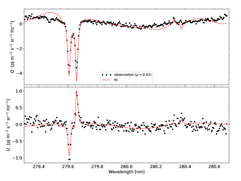
Figure 9: Stokes $Q$ (top panel) and $U$ (bottom panel) profiles for the observation (black dots) and the best inversion fit (red curve) for one pixel in CLASP2 showing an antisymmetric $U$ signal. The inversion needs to take into account the gradients of the horizontal components of the macroscopic velocity. Image reproduced with permission from Li et al. [116].

Several pixels in quiet regions observed by CLASP2 showed antisymmetric Stokes $U$ signals around the center of the k line. In a 1D model atmosphere, such profiles can only be synthesized by introducing a vertical gradient in the horizontal component of the macroscopic velocity [116]. Fig. 9 shows the observed linear polarization profiles in one such pixel from the quiet Sun observation for a LOS with $\mu=0.42$, as well as the corresponding fit from the inversion. A horizontal velocity difference of about 5 $\rm km\,s^{-1}$ between the upper and lower chromosphere was inferred from this inversion. Antisymmetric Stokes $U$ profiles were detected in only a few pixels, suggesting that such horizontal velocity gradients may not be significant in most regions of the quiet solar chromosphere.

7.3.3 Degeneracies and ambiguities

Degeneracies among the ad-hoc radiation tensor components ${J^{\dagger}}^{K}_{Q}$ and the magnetic field vector has been reported by Li et al. [116]. As it happens with other degeneracies, changes in some of the parameters can be partially compensated with changes in others. However, it is important to emphasize that there is some degree of degeneracy, but not complete degeneracy. For instance, the longitudinal component of the magnetic field modulates both Stokes $V$, the coupling between Stokes $Q$ and $U$ in the RT equations, and the depolarization of the linear polarization of the line wings. Regarding the ad-hoc radiation tensor components, they are added to the proper tensor components resulting from the 1D calculations in each iteration of the forward modeling. Although they get “mixed” with the anisotropy calculated in the vertical reference frame when there is a non-vertical magnetic field, the solution of the 1D RT problem must be self-consistent and physical, and produce emergent profiles that fit the observation. In summary, the physics of the problem imposes some constraints on the mentioned degeneracy. Thus, not all combinations of these parameters are possible, although it is very difficult to demonstrate it formally when RT, scattering polarization, PRD effects, and the Hanle effect are accounted for.

An alternative method to constrain the degeneracy is to estimate the ad-hoc radiation tensor components from the intensity map, as demonstrated by Zeuner et al. [214, 215] in their investigations on the scattering polarization of the Sr I 4607 Å line. However, while this approach may be effective for photospheric lines, it does not yield good results for chromospheric lines.

It is important to mention that the ad-hoc radiation tensor components are not intrinsic parameters in the RT calculations. They are exclusively introduced to mimic the effect of horizontal RT, which cannot be taken into account in 1D inversion codes. These contributions can, in principle, be fully accounted for through full 3D RT calculations [198]. A 3D inversion framework has recently been developed by Štěpán et al. [202] and applied to the synthesized Stokes profiles of the Mg II k line in a prominence model [203]. Currently, this approach is limited to CRD, but there is an ongoing effort to extend it to include coherent scattering in the line wings and to apply it to the CLASP2.1 observations.

Regarding the ambiguities in the direction of the magnetic field vector, in contrast to the well known 180^∘ azimuthal ambiguity of the Zeeman effect [130], the ambiguity suffered by the Hanle effect is associated with the magnetic field vector in the local vertical reference frame [see the Hanle diagrams in 110]. In the saturated regime of the Hanle effect, it is known as the Van Vleck ambiguity, which leads to multiple possible solutions for the magnetic field vector (see Asensio Ramos et al. 13 for the He I triplet at around 1083.0 nm, and Casini et al. 42 for the forbidden coronal lines). However, in the case of the Mg II k line, the ambiguity is more complex due to the significant influence of the M-O and PRD effects on the linear polarization, particularly in the wings. This complexity has been demonstrated through the inversions by Li et al. [116], whose results show that different combinations of magnetic field inclination and azimuth can produce very similar Stokes $Q$ and $U$ profiles, successfully fitting the CLASP2 observations.

8 Summary and future perspectives

The polarization signals of the Mg II h and k lines have demonstrated significant potential for diagnosing the magnetic field in the solar chromosphere, which is key to address some of the still open questions in solar physics. The CLASP2 and CLASP2.1 sounding rocket experiments successfully acquired spectropolarimetric observations of these lines. Analyses built on these unprecedented data have demonstrated the capability to infer magnetic fields from such observations [86, 115, 116, 117, 172, 88, 4].

The WFA provides a fast estimation of the longitudinal component of the magnetic field, while non-LTE inversion techniques can retrieve the magnetic field vector from the full Stokes profiles. However, the non-LTE inversions require accounting for a plethora of physical ingredients which make them computationally heavy.

To accelerate the inversion process, several approaches have been proposed. These include database-based inversions [161], convolutional neural networks for rapid computation of RFs [45], or graph networks for the prediction of departure coefficients [195]. For a comprehensive review on machine learning applications in Stokes inversions, see Asensio Ramos et al. [14].

Currently, non-LTE inversions of the Mg II h and k lines are limited to 1D atmospheric models. To reproduce the observed Stokes profiles, ad-hoc radiation tensor components need to be introduced in order to mimic the contribution from the 3D effects. These ad-hoc tensor components introduce degeneracies among model parameters. Overcoming this limitation requires a fully 3D inversion framework. At present, such a framework has been developed only under the assumption of CRD, though efforts are underway to partially extend this approach. Moreover, neural fields offer a promising way to represent model parameters in the 3D inversion [12, 65].

Finally, we emphasize the potential of future space missions with CLASP2-like capabilities to advance our understanding of magnetic fields in the solar chromosphere. Moreover, in addition to the lines present in the CALSP2/2.1 spectral range [4], several Fe II lines are located in the wavelength range between 250 and 278 nm [94]. Simultaneous observation of all these lines alongside the Mg II h and k lines would facilitate magnetic diagnostics spanning from the solar photosphere to the upper chromosphere [3, 2, 4].

Acknowledgements

H.L. acknowledges the support from the National Key R&D Program of China (2021YFA1600500, 2021YFA1600503), and the National Natural Science Foundation of China under grant No. 12473051. T.P.A. and J.T.B. acknowledge support from the Agencia Estatal de Investigación del Ministerio de Ciencia, Innovación y Universidades (MCIU/AEI) under grant “Polarimetric Inference of Magnetic Fields” and the European Regional Development Fund (ERDF) with reference PID2022-136563NB-I00/10.13039/501100011033. T.P.A.’s participation in the publication is part of the Project RYC2021-034006-I, funded by MICIN/AEI/10.13039/501100011033, and the European Union “NextGenerationEU”/RTRP.

Conflicts of interest

All authors declare that they have no conflicts of interest.

References

- \bibcommenthead
- Afonso Delgado et al. [2023a] Afonso Delgado D, del Pino Alemán T, Trujillo Bueno J (2023a) Formation of the Mg II h and k Polarization Profiles in a Solar Plage Model and Their Suitability to Infer Magnetic Fields. The Astrophysical Journal 942(2):60. 10.3847/1538-4357/aca669, arXiv:2211.14044 [astro-ph.SR]
- Afonso Delgado et al. [2023b] Afonso Delgado D, del Pino Alemán T, Trujillo Bueno J (2023b) Magnetic Field Information in the Near-ultraviolet Fe II Lines of the CLASP2 Space Experiment. The Astrophysical Journal 954(2):218. 10.3847/1538-4357/ace4c8, arXiv:2307.01641 [astro-ph.SR]
- Afonso Delgado et al. [2023c] Afonso Delgado D, del Pino Alemán T, Trujillo Bueno J (2023c) The Magnetic Sensitivity of the (250-278 nm) Fe II Polarization Spectrum. The Astrophysical Journal 948(2):86. 10.3847/1538-4357/acc399, arXiv:2303.07066 [astro-ph.SR]
- Afonso Delgado et al. [2025] Afonso Delgado D, del Pino Alemán T, Trujillo Bueno J, et al (2025) Determining the Magnetic Field of Active Region Plages Using the Whole CLASP2/2.1 Spectral Window. The Astrophysical Journal 991(2):164. 10.3847/1538-4357/adfcd4, arXiv:2508.14347 [astro-ph.SR]
- Alsina Ballester et al. [2016] Alsina Ballester E, Belluzzi L, Trujillo Bueno J (2016) The Magnetic Sensitivity of the Mg II k Line to the Joint Action of Hanle, Zeeman, and Magneto-optical Effects. The Astrophysical Journal Letters 831(2):L15. 10.3847/2041-8205/831/2/L15, arXiv:1610.00649 [astro-ph.SR]
- Alsina Ballester et al. [2017] Alsina Ballester E, Belluzzi L, Trujillo Bueno J (2017) The Transfer of Resonance Line Polarization with Partial Frequency Redistribution in the General Hanle-Zeeman Regime. The Astrophysical Journal Letters 836(1):6. 10.3847/1538-4357/836/1/6, arXiv:1609.05723 [astro-ph.SR]
- Alsina Ballester et al. [2022] Alsina Ballester E, Belluzzi L, Trujillo Bueno J (2022) The transfer of polarized radiation in resonance lines with partial frequency redistribution, J-state interference, and arbitrary magnetic fields. A radiative transfer code and useful approximations. Astronomy and Astrophysics 664:A76. 10.1051/0004-6361/202142934, arXiv:2204.12523 [astro-ph.SR]
- Anan et al. [2021] Anan T, Schad TA, Kitai R, et al (2021) Measurements of Photospheric and Chromospheric Magnetic Field Structures Associated with Chromospheric Heating over a Solar Plage Region. The Astrophysical Journal 921(1):39. 10.3847/1538-4357/ac1b9c, arXiv:2108.07907 [astro-ph.SR]
- Anan et al. [2024] Anan T, Casini R, Uitenbroek H, et al (2024) Magnetic diffusion in solar atmosphere produces measurable electric fields. Nature Communications 15(1):8811. 10.1038/s41467-024-53102-x, arXiv:2410.09221 [astro-ph.SR]
- Anderson [1949] Anderson PW (1949) Pressure Broadening in the Microwave and Infra-Red Regions. Physical Review 76(5):647–661. 10.1103/PhysRev.76.647
- Aschwanden et al. [2007] Aschwanden MJ, Winebarger A, Tsiklauri D, et al (2007) The Coronal Heating Paradox. The Astrophysical Journal 659(2):1673–1681. 10.1086/513070
- Asensio Ramos [2023] Asensio Ramos A (2023) Tomographic Reconstruction of the Solar K-Corona Using Neural Fields. Solar Physics 298(11):135. 10.1007/s11207-023-02226-2
- Asensio Ramos et al. [2008] Asensio Ramos A, Trujillo Bueno J, Land i Degl’Innocenti E (2008) Advanced Forward Modeling and Inversion of Stokes Profiles Resulting from the Joint Action of the Hanle and Zeeman Effects. The Astrophysical Journal 683(1):542–565. 10.1086/589433, arXiv:0804.2695 [astro-ph]
- Asensio Ramos et al. [2023] Asensio Ramos A, Cheung MCM, Chifu I, et al (2023) Machine learning in solar physics. Living Reviews in Solar Physics 20(1):4. 10.1007/s41116-023-00038-x, arXiv:2306.15308 [astro-ph.SR]
- Asplund et al. [2009] Asplund M, Grevesse N, Sauval AJ, et al (2009) The Chemical Composition of the Sun. Annual Review of Astronomy and Astrophysics 47(1):481–522. 10.1146/annurev.astro.46.060407.145222, arXiv:0909.0948 [astro-ph.SR]
- Auer et al. [1980] Auer LH, Rees DE, Stenflo JO (1980) Resonance-Line Polarization - Part Six - Line Wing Transfer Calculations Including Excited State Interference. Astronomy and Astrophysics 88:302
- Baranger [1958] Baranger M (1958) Problem of Overlapping Lines in the Theory of Pressure Broadening. Physical Review 111(2):494–504. 10.1103/PhysRev.111.494
- Belluzzi and Trujillo Bueno [2011] Belluzzi L, Trujillo Bueno J (2011) The Impact of Quantum Interference between Different J-levels on Scattering Polarization in Spectral Lines. The Astrophysical Journal 743(1):3. 10.1088/0004-637X/743/1/3, arXiv:1109.0424 [astro-ph.SR]
- Belluzzi and Trujillo Bueno [2012] Belluzzi L, Trujillo Bueno J (2012) The Polarization of the Solar Mg II h and k Lines. The Astrophysical Journal Letters 750(1):L11. 10.1088/2041-8205/750/1/L11, arXiv:1203.4351 [astro-ph.SR]
- Belluzzi and Trujillo Bueno [2014] Belluzzi L, Trujillo Bueno J (2014) The transfer of resonance line polarization with partial frequency redistribution and J-state interference. Theoretical approach and numerical methods. Astronomy and Astrophysics 564:A16. 10.1051/0004-6361/201321598, arXiv:1403.1701 [astro-ph.SR]
- Belluzzi et al. [2012] Belluzzi L, Trujillo Bueno J, Štěpán J (2012) The Scattering Polarization of the Ly Lines of H I and He II Taking into Account Partial Frequency Redistribution and J-state Interference Effects. The Astrophysical Journal Letters 755(1):L2. 10.1088/2041-8205/755/1/L2, arXiv:1207.0415 [astro-ph.SR]
- Belluzzi et al. [2024] Belluzzi L, Riva S, Janett G, et al (2024) Accurate modeling of the forward-scattering Hanle effect in the chromospheric Ca I 4227 Å line. Astronomy and Astrophysics 691:A278. 10.1051/0004-6361/202450178, arXiv:2404.00104 [astro-ph.SR]
- Benedusi et al. [2023] Benedusi P, Riva S, Zulian P, et al (2023) Scalable matrix-free solver for 3D transfer of polarized radiation in stellar atmospheres. Journal of Computational Physics 479:112013. 10.1016/j.jcp.2023.112013
- Bohlin et al. [1980] Bohlin JD, Frost KJ, Burr PT, et al (1980) Solar Maximum Mission. Solar Physics 65(1):5–14. 10.1007/BF00151380
- Bommier [1980] Bommier V (1980) Quantum theory of the Hanle effect. II - Effect of level-crossings and anti-level-crossings on the polarization of the D3 helium line of solar prominences. Astronomy and Astrophysics 87(1-2):109–120
- Bommier [1997a] Bommier V (1997a) Master equation theory applied to the redistribution of polarized radiation, in the weak radiation field limit. I. Zero magnetic field case. Astronomy and Astrophysics 328:706–725
- Bommier [1997b] Bommier V (1997b) Master equation theory applied to the redistribution of polarized radiation, in the weak radiation field limit. II. Arbitrary magnetic field case. Astronomy and Astrophysics 328:726–751
- Bommier [2017] Bommier V (2017) Master equation theory applied to the redistribution of polarized radiation in the weak radiation field limit. V. The two-term atom. Astronomy and Astrophysics 607:A50. 10.1051/0004-6361/201630169, arXiv:1708.05579 [astro-ph.SR]
- Bommier and Sahal-Brechot [1978] Bommier V, Sahal-Brechot S (1978) Quantum theory of the Hanle effect: calculations of the Stokes parameters of the D3 helium line for quiescent prominences. Astronomy and Astrophysics 69(1):57–64
- Borrero et al. [2019] Borrero JM, Pastor Yabar A, Rempel M, et al (2019) Combining magnetohydrostatic constraints with Stokes profiles inversions. I. Role of boundary conditions. Astronomy and Astrophysics 632:A111. 10.1051/0004-6361/201936367, arXiv:1910.14131 [astro-ph.SR]
- Bose et al. [2024] Bose S, De Pontieu B, Hansteen V, et al (2024) Chromospheric and coronal heating in an active region plage by dissipation of currents from braiding. Nature Astronomy 8:697–705. 10.1038/s41550-024-02241-8, arXiv:2211.08579 [astro-ph.SR]
- Bryans et al. [2020] Bryans P, McIntosh SW, Brooks DH, et al (2020) Investigating the Chromospheric Footpoints of the Solar Wind. The Astrophysical Journal Letters 905(2):L33. 10.3847/2041-8213/abce69
- Carlsson and Leenaarts [2012] Carlsson M, Leenaarts J (2012) Approximations for radiative cooling and heating in the solar chromosphere. Astronomy and Astrophysics 539:A39. 10.1051/0004-6361/201118366, arXiv:1202.2996 [astro-ph.SR]
- Carlsson et al. [2019] Carlsson M, De Pontieu B, Hansteen VH (2019) New View of the Solar Chromosphere. Annual Review of Astronomy and Astrophysics 57:189–226. 10.1146/annurev-astro-081817-052044
- Casini [2005] Casini R (2005) Resonance scattering formalism for the hydrogen lines in the presence of magnetic and electric fields. Physical Review A 71(6):062505. 10.1103/PhysRevA.71.062505
- Casini and Judge [1999] Casini R, Judge PG (1999) Spectral Lines for Polarization Measurements of the Coronal Magnetic Field. II. Consistent Treatment of the Stokes Vector forMagnetic-Dipole Transitions. The Astrophysical Journal 522(1):524–539. 10.1086/307629
- Casini and Landi Degl’Innocenti [2008] Casini R, Landi Degl’Innocenti E (2008) Astrophysical Plasmas. In: Fujimoto T, Iwamae A (eds) Plasma Polarization Spectroscopy, vol 44. p 247, 10.1007/978-3-540-73587-8_12
- Casini and Manso Sainz [2016] Casini R, Manso Sainz R (2016) Frequency Redistribution of Polarized Light in the -Type Multi-Term Polarized Atom. The Astrophysical Journal 824(2):135. 10.3847/0004-637X/824/2/135, arXiv:1602.07173 [astro-ph.SR]
- Casini et al. [2014] Casini R, Landi Degl’Innocenti M, Manso Sainz R, et al (2014) Frequency Redistribution Function for the Polarized Two-term Atom. The Astrophysical Journal 791(2):94. 10.1088/0004-637X/791/2/94, arXiv:1406.6129 [astro-ph.SR]
- Casini et al. [2017a] Casini R, del Pino Alemán T, Manso Sainz R (2017a) A Note on the Radiative and Collisional Branching Ratios in Polarized Radiation Transport with Coherent Scattering. The Astrophysical Journal 835:114. 10.3847/1538-4357/835/2/114, arXiv:1612.03440 [astro-ph.SR]
- Casini et al. [2017b] Casini R, del Pino Alemán T, Manso Sainz R (2017b) Explicit Form of the Radiative and Collisional Branching Ratios in Polarized Radiation Transport with Coherent Scattering. The Astrophysical Journal 848:99. 10.3847/1538-4357/aa8a73, arXiv:1709.00126 [astro-ph.SR]
- Casini et al. [2017c] Casini R, White SM, Judge PG (2017c) Magnetic Diagnostics of the Solar Corona: Synthesizing Optical and Radio Techniques. Space Science Reviews 210(1-4):145–181. 10.1007/s11214-017-0400-6
- Casini et al. [2025] Casini R, Manso Sainz R, López Ariste A, et al (2025) A Unifying Polarization Formalism for Electric and Magnetic Multipole Interactions. The Astrophysical Journal 980(1):67. 10.3847/1538-4357/ad7677, arXiv:2409.01197 [physics.atom-ph]
- Centeno et al. [2010] Centeno R, Trujillo Bueno J, Asensio Ramos A (2010) On the Magnetic Field of Off-limb Spicules. The Astrophysical Journal 708(2):1579–1584. 10.1088/0004-637X/708/2/1579, arXiv:0911.3149 [astro-ph.SR]
- Centeno et al. [2022a] Centeno R, Flyer N, Mukherjee L, et al (2022a) Convolutional Neural Networks and Stokes Response Functions. The Astrophysical Journal 925(2):176. 10.3847/1538-4357/ac402f, arXiv:2112.03802 [astro-ph.IM]
- Centeno et al. [2022b] Centeno R, Rempel M, Casini R, et al (2022b) Effects of Spectral Resolution on Simple Magnetic Field Diagnostics of the Mg II H and K Lines. The Astrophysical Journal 936(2):115. 10.3847/1538-4357/ac886f, arXiv:2208.07507 [astro-ph.SR]
- Chen et al. [2020] Chen B, Shen C, Gary DE, et al (2020) Measurement of magnetic field and relativistic electrons along a solar flare current sheet. Nature Astronomy 4:1140–1147. 10.1038/s41550-020-1147-7, arXiv:2005.12757 [astro-ph.SR]
- Chen et al. [2025] Chen X, Chen B, Yu S, et al (2025) Measuring the Magnetic Field of a Coronal Mass Ejection from the Low to Middle Corona. The Astrophysical Journal Letters 990(2):L50. 10.3847/2041-8213/adfa71, arXiv:2508.08970 [astro-ph.SR]
- Chen et al. [2021] Chen Y, Li W, Tian H, et al (2021) Forward Modeling of Solar Coronal Magnetic-field Measurements Based on a Magnetic-field-induced Transition in Fe X. The Astrophysical Journal 920(2):116. 10.3847/1538-4357/ac1792, arXiv:2107.11783 [astro-ph.SR]
- Cohen-Tannoudji and Kastler [1966] Cohen-Tannoudji C, Kastler A (1966) Optical Pumping. Progess in Optics 5:1–81. 10.1016/S0079-6638(08)70450-5
- da Silva Santos et al. [2018] da Silva Santos JM, de la Cruz Rodríguez J, Leenaarts J (2018) Temperature constraints from inversions of synthetic solar optical, UV, and radio spectra. Astronomy and Astrophysics 620:A124. 10.1051/0004-6361/201833664, arXiv:1806.06682 [astro-ph.SR]
- da Silva Santos et al. [2020] da Silva Santos JM, de la Cruz Rodríguez J, Leenaarts J, et al (2020) The multi-thermal chromosphere. Inversions of ALMA and IRIS data. Astronomy and Astrophysics 634:A56. 10.1051/0004-6361/201937117, arXiv:1912.09886 [astro-ph.SR]
- da Silva Santos et al. [2023] da Silva Santos JM, Reardon K, Cauzzi G, et al (2023) Magnetic Fields in Solar Plage Regions: Insights from High-sensitivity Spectropolarimetry. The Astrophysical Journal Letters 954(2):L35. 10.3847/2041-8213/acf21f, arXiv:2308.10983 [astro-ph.SR]
- de la Cruz Rodríguez and van Noort [2017] de la Cruz Rodríguez J, van Noort M (2017) Radiative Diagnostics in the Solar Photosphere and Chromosphere. Space Science Reviews 210(1-4):109–143. 10.1007/s11214-016-0294-8, arXiv:1609.08324 [astro-ph.SR]
- de la Cruz Rodríguez et al. [2016] de la Cruz Rodríguez J, Leenaarts J, Asensio Ramos A (2016) Non-LTE Inversions of the Mg II h & k and UV Triplet Lines. The Astrophysical Journal Letters 830(2):L30. 10.3847/2041-8205/830/2/L30, arXiv:1609.09527 [astro-ph.SR]
- de la Cruz Rodríguez et al. [2019] de la Cruz Rodríguez J, Leenaarts J, Danilovic S, et al (2019) STiC: A multiatom non-LTE PRD inversion code for full-Stokes solar observations. Astronomy and Astrophysics 623:A74. 10.1051/0004-6361/201834464, arXiv:1810.08441 [astro-ph.SR]
- De Pontieu et al. [2003] De Pontieu B, Tarbell T, Erdélyi R (2003) Correlations on Arcsecond Scales between Chromospheric and Transition Region Emission in Active Regions. The Astrophysical Journal 590(1):502–518. 10.1086/374928
- De Pontieu et al. [2014] De Pontieu B, Title AM, Lemen JR, et al (2014) The Interface Region Imaging Spectrograph (IRIS). Solar Physics 289(7):2733–2779. 10.1007/s11207-014-0485-y, arXiv:1401.2491 [astro-ph.SR]
- De Pontieu et al. [2021] De Pontieu B, Polito V, Hansteen V, et al (2021) A New View of the Solar Interface Region from the Interface Region Imaging Spectrograph (IRIS). Solar Physics 296(5):84. 10.1007/s11207-021-01826-0, arXiv:2103.16109 [astro-ph.SR]
- del Pino Alemán et al. [2016] del Pino Alemán T, Casini R, Manso Sainz R (2016) Magnetic Diagnostics of the Solar Chromosphere with the Mg II h-k Lines. The Astrophysical Journal Letters 830(2):L24. 10.3847/2041-8205/830/2/L24, arXiv:1607.05683 [astro-ph.SR]
- del Pino Alemán et al. [2020] del Pino Alemán T, Trujillo Bueno J, Casini R, et al (2020) The Magnetic Sensitivity of the Resonance and Subordinate Lines of Mg II in the Solar Chromosphere. The Astrophysical Journal 891(1):91. 10.3847/1538-4357/ab6bc9, arXiv:2004.09176 [astro-ph.SR]
- del Pino Alemán et al. [2025] del Pino Alemán T, Alsina Ballester E, Trujillo Bueno J, et al (2025) The Impact of the Angle-average Approximation in the Partial Frequency Redistribution Modeling of the Mg II h–k Doublet Stokes Profiles. The Astrophysical Journal 978(1):27. 10.3847/1538-4357/ad95f7
- del Toro Iniesta [2003] del Toro Iniesta JC (2003) Introduction to Spectropolarimetry. Cambridge Univ. Press, Cambridge
- del Toro Iniesta and Ruiz Cobo [2016] del Toro Iniesta JC, Ruiz Cobo B (2016) Inversion of the radiative transfer equation for polarized light. Living Reviews in Solar Physics 13(1):4. 10.1007/s41116-016-0005-2, arXiv:1610.10039 [astro-ph.SR]
- Díaz Baso et al. [2025] Díaz Baso CJ, Asensio Ramos A, de la Cruz Rodríguez J, et al (2025) Exploring spectropolarimetric inversions using neural fields: Solar chromospheric magnetic field under the weak-field approximation. Astronomy and Astrophysics 693:A170. 10.1051/0004-6361/202452172, arXiv:2409.05156 [astro-ph.SR]
- Domke and Hubeny [1988] Domke H, Hubeny I (1988) Scattering of Polarized Light in Spectral Lines with Partial Frequency Redistribution: General Redistribution Matrix. The Astrophysical Journal 334:527. 10.1086/166857
- Esteban Pozuelo et al. [2023] Esteban Pozuelo S, Asensio Ramos A, de la Cruz Rodríguez J, et al (2023) Estimating the longitudinal magnetic field in the chromosphere of quiet-Sun magnetic concentrations. Astronomy and Astrophysics 672:A141. 10.1051/0004-6361/202245267, arXiv:2302.04258 [astro-ph.SR]
- Esteban Pozuelo et al. [2025] Esteban Pozuelo S, Asensio Ramos A, Trujillo Bueno J, et al (2025) Study of an active region prominence using spectropolarimetric data in the He I D3 multiplet. Astronomy and Astrophysics 696:A109. 10.1051/0004-6361/202452439, arXiv:2503.03670 [astro-ph.SR]
- Fano [1957] Fano U (1957) Description of States in Quantum Mechanics by Density Matrix and Operator Techniques. Reviews of Modern Physics 29(1):74–93. 10.1103/RevModPhys.29.74
- Fiutak and Kranendonk [1962] Fiutak J, Kranendonk JV (1962) Impact Theory of Raman Line Broadening. Canadian Journal of Physics 40(9):1085–1100. 10.1139/p62-117
- Fontenla et al. [1993] Fontenla JM, Avrett EH, Loeser R (1993) Energy balance in the solar transition region. III - Helium emission in hydrostatic, constant-abundance models with diffusion. The Astrophysical Journal 406:319–345. 10.1086/172443
- Frutiger et al. [2000] Frutiger C, Solanki SK, Fligge M, et al (2000) Properties of the solar granulation obtained from the inversion of low spatial resolution spectra. Astronomy and Astrophysics 358:1109–1121
- Gandorfer [2000] Gandorfer A (2000) The Second Solar Spectrum: A high spectral resolution polarimetric survey of scattering polarization at the solar limb in graphical representation. Volume I: 4625 Å to 6995 Å. Hochschulverlag, Zurich
- Gandorfer [2002] Gandorfer A (2002) The Second Solar Spectrum: A high spectral resolution polarimetric survey of scattering polarization at the solar limb in graphical representation. Volume II: 3910 Å to 4630 Å. Hochschulverlag, Zurich
- Gandorfer [2005] Gandorfer A (2005) The Second Solar Spectrum: A high spectral resolution polarimetric survey of scattering polarization at the solar limb in graphical representation. Volume III: 3160 Å to 3915 Å. Hochschulverlag, Zurich
- Gandorfer et al. [2004] Gandorfer AM, Steiner HPPP, Aebersold F, et al (2004) Solar polarimetry in the near UV with the Zurich Imaging Polarimeter ZIMPOL II. Astronomy and Astrophysics 422:703–708. 10.1051/0004-6361:20040254
- Gary [2001] Gary GA (2001) Plasma Beta above a Solar Active Region: Rethinking the Paradigm. Solar Physics 203(1):71–86. 10.1023/A:1012722021820
- Guerreiro et al. [2024] Guerreiro N, Janett G, Riva S, et al (2024) Modeling the scattering polarization in the solar Ca I 4227Å line with angle-dependent PRD effects and bulk velocities. Astronomy and Astrophysics 683:A207. 10.1051/0004-6361/202346399
- Hale [1908] Hale GE (1908) On the Probable Existence of a Magnetic Field in Sun-Spots. The Astrophysical Journal 28:315. 10.1086/141602
- Hanle [1924] Hanle W (1924) Über magnetische Beeinflussung der Polarisation der Resonanzfluoreszenz. Zeitschrift fur Physik 30(1):93–105. 10.1007/BF01331827
- Happer [1972] Happer W (1972) Optical Pumping. Reviews of Modern Physics 44(2):169–249. 10.1103/RevModPhys.44.169
- Henze and Stenflo [1987] Henze W, Stenflo JO (1987) Polarimetry in the Mg II h and k lines. Solar Physics 111(2):243–254. 10.1007/BF00148517
- Hofmann et al. [2025] Hofmann RA, Afonso Delgado D, Centeno R, et al (2025) Using the Hanle Effect in Mg II k to Quantify the Open Flux above the Solar Poles. The Astrophysical Journal 990(2):134. 10.3847/1538-4357/adf228
- Hummer [1962] Hummer DG (1962) Non-coherent scattering: I. The redistribution function with Doppler broadening. Monthly Notices of the Royal Astronomical Society 125:21–37. 10.1093/mnras/125.1.21
- Ishikawa et al. [2014] Ishikawa R, Asensio Ramos A, Belluzzi L, et al (2014) On the Inversion of the Scattering Polarization and the Hanle Effect Signals in the Hydrogen Ly Line. The Astrophysical Journal 787(2):159. 10.1088/0004-637X/787/2/159, arXiv:1404.0786 [astro-ph.SR]
- Ishikawa et al. [2021] Ishikawa R, Trujillo Bueno J, del Pino Alemán T, et al (2021) Mapping solar magnetic fields from the photosphere to the base of the corona. Science Advances 7(8):eabe8406. 10.1126/sciadv.abe8406, arXiv:2103.01583 [astro-ph.SR]
- Ishikawa et al. [2023] Ishikawa R, Trujillo Bueno J, Alsina Ballester E, et al (2023) Evidence for the Operation of the Hanle and Magneto-optical Effects in the Scattering Polarization Signals Observed by CLASP2 across the Mg II h and k Lines. The Astrophysical Journal 945(2):125. 10.3847/1538-4357/acb64e, arXiv:2302.03303 [astro-ph.SR]
- Ishikawa et al. [2025] Ishikawa R, Trujillo Bueno J, McKenzie DE, et al (2025) Determining the Magnetic Field in the Atmosphere of a Solar Active Region Observed by the CLASP2.1 Sounding Rocket Experiment. arXiv e-prints arXiv:2507.09878. arXiv:2507.09878 [astro-ph.SR]
- Ivanov [1991] Ivanov VV (1991) Analytical Methods of Line Formation Theory - are they Still Alive. In: Crivellari L, Hubeny I, Hummer DG (eds) Stellar Atmospheres - Beyond Classical Models, p 81, 10.1007/978-94-011-3554-2_9
- Janett et al. [2021] Janett G, Alsina Ballester E, Guerreiro N, et al (2021) Modeling the scattering polarization of the solar Ca I 4227 Å line with angle-dependent partial frequency redistribution. Astronomy and Astrophysics 655:A13. 10.1051/0004-6361/202141549, arXiv:2110.11990 [astro-ph.SR]
- Jaume Bestard et al. [2021] Jaume Bestard J, Trujillo Bueno J, Štěpán J, et al (2021) The Effects of Three-dimensional Radiative Transfer on the Resonance Polarization of the Ca I 4227 Å Line. Astronomy and Astrophysics 909(2):183. 10.3847/1538-4357/abd94a, arXiv:2101.04421 [astro-ph.SR]
- Jefferies et al. [1989] Jefferies J, Lites BW, Skumanich A (1989) Transfer of Line Radiation in a Magnetic Field. The Astrophysical Journal 343:920. 10.1086/167762
- Johnson et al. [1953] Johnson FS, Purcell JD, Tousey R, et al (1953) A New Photograph of the MG II Doublet at 2800 A in the Sun. The Astrophysical Journal 117:238. 10.1086/145685
- Judge et al. [2021] Judge P, Rempel M, Ezzeddine R, et al (2021) Measuring the Magnetic Origins of Solar Flares, Coronal Mass Ejections, and Space Weather. The Astrophysical Journal 917(1):27. 10.3847/1538-4357/ac081f, arXiv:2106.07786 [astro-ph.SR]
- Judge et al. [2022] Judge P, Bryans P, Casini R, et al (2022) Optimal Spectral Lines for Measuring Chromospheric Magnetic Fields. The Astrophysical Journal 941(2):159. 10.3847/1538-4357/aca2a5, arXiv:2211.07770 [astro-ph.SR]
- Judge et al. [2024] Judge P, Kleint L, Casini R, et al (2024) Magnetic Fields and Plasma Heating in the Sun’s Atmosphere. The Astrophysical Journal 960(2):129. 10.3847/1538-4357/ad0780, arXiv:2311.01286 [astro-ph.SR]
- Kano et al. [2017] Kano R, Trujillo Bueno J, Winebarger A, et al (2017) Discovery of Scattering Polarization in the Hydrogen Ly Line of the Solar Disk Radiation. The Astrophysical Journal Letters 839(1):L10. 10.3847/2041-8213/aa697f, arXiv:1704.03228 [astro-ph.SR]
- Kleint and Gandorfer [2017] Kleint L, Gandorfer A (2017) Prospects of Solar Magnetometry—From Ground and in Space. Space Science Reviews 210(1-4):397–426. 10.1007/s11214-015-0208-1, arXiv:1510.03763 [astro-ph.SR]
- Kobayashi et al. [2012] Kobayashi K, Kano R, Trujillo Bueno J, et al (2012) The Chromospheric Lyman-Alpha SpectroPolarimeter: CLASP. In: Golub L, De Moortel I, Shimizu T (eds) Fifth Hinode Science Meeting, p 233
- Kramida et al. [2024] Kramida A, Yu. Ralchenko, Reader J, et al (2024) NIST Atomic Spectra Database (version 5.12), [Online]. Available:http://physics.nist.gov/asd. National Institute of Standards and Technology, Gaithersburg, MD., https://doi.org/10.18434/T4W30F
- Lagg et al. [2017] Lagg A, Lites B, Harvey J, et al (2017) Measurements of Photospheric and Chromospheric Magnetic Fields. Space Science Reviews 210(1-4):37–76. 10.1007/s11214-015-0219-y, arXiv:1510.06865 [astro-ph.SR]
- Landi et al. [2020] Landi E, Hutton R, Brage T, et al (2020) Hinode/EIS Measurements of Active-region Magnetic Fields. The Astrophysical Journal 904(2):87. 10.3847/1538-4357/abbf54, arXiv:2008.03532 [astro-ph.SR]
- Landi Degl’Innocenti [1983a] Landi Degl’Innocenti E (1983a) Polarization in spectral lines. I: A Unifying Theoretical Approach. Solar Physics 85(1):3–31. 10.1007/BF00148254
- Landi Degl’Innocenti [1983b] Landi Degl’Innocenti E (1983b) Polarization in spectral lines. II: A Classification Scheme for Solar Observatories. Solar Physics 85(1):33–40. 10.1007/BF00148255
- Landi Degl’Innocenti [1984] Landi Degl’Innocenti E (1984) Polarization in Spectral Lines - Part Three - Resonance Polarization in the Non-Magnetic Collisionless Regime. Solar Physics 91(1):1–26. 10.1007/BF00213606
- Landi Degl’Innocenti [1985] Landi Degl’Innocenti E (1985) Polarization in spectral lines. IV: Resonance polarization in the Hanle effect, collisionless regime. Solar Physics 102(1-2):1–20. 10.1007/BF00154032
- Landi Degl’Innocenti and Landi Degl’Innocenti [1972] Landi Degl’Innocenti E, Landi Degl’Innocenti M (1972) Quantum Theory of Line Formation in a Magnetic Field. Solar Physics 27:319. 10.1007/BF00153104
- Landi Degl’Innocenti and Landi Degl’Innocenti [1973] Landi Degl’Innocenti E, Landi Degl’Innocenti M (1973) A Perturbative Solution of the Transfer Equations for the Stokes Parameters in a Magnetic Field. Solar Physics 31:299. 10.1007/BF00152807
- Landi Degl’Innocenti and Landi Degl’Innocenti [1977] Landi Degl’Innocenti E, Landi Degl’Innocenti M (1977) Response function for magnetic lines. Astronomy and Astrophysics 56:111–115
- Landi Degl’Innocenti and Landolfi [2004] Landi Degl’Innocenti E, Landolfi M (2004) Polarization in Spectral Lines, vol 307. KluwerAcademic, Dordrecht, 10.1007/978-1-4020-2415-3
- Leenaarts et al. [2012] Leenaarts J, Pereira T, Uitenbroek H (2012) Fast approximation of angle-dependent partial redistribution in moving atmospheres. Astronomy and Astrophysics 543:A109. 10.1051/0004-6361/201219394, arXiv:1205.5110 [astro-ph.SR]
- Leenaarts et al. [2013a] Leenaarts J, Pereira TMD, Carlsson M, et al (2013a) The Formation of IRIS Diagnostics. I. A Quintessential Model Atom of Mg II and General Formation Properties of the Mg II h&k Lines. The Astrophysical Journal 772(2):89. 10.1088/0004-637X/772/2/89, arXiv:1306.0668 [astro-ph.SR]
- Leenaarts et al. [2013b] Leenaarts J, Pereira TMD, Carlsson M, et al (2013b) The Formation of IRIS Diagnostics. II. The Formation of the Mg II h&k Lines in the Solar Atmosphere. The Astrophysical Journal 772(2):90. 10.1088/0004-637X/772/2/90, arXiv:1306.0671 [astro-ph.SR]
- Li et al. [2022] Li H, del Pino Alemán T, Trujillo Bueno J, et al (2022) TIC: A Stokes Inversion Code for Scattering Polarization with Partial Frequency Redistribution and Arbitrary Magnetic Fields. The Astrophysical Journal 933(2):145. 10.3847/1538-4357/ac745c, arXiv:2205.15666 [astro-ph.SR]
- Li et al. [2023] Li H, del Pino Alemán T, Trujillo Bueno J, et al (2023) Tomography of a Solar Plage with the Tenerife Inversion Code. The Astrophysical Journal 945(2):144. 10.3847/1538-4357/acb76e, arXiv:2301.12792 [astro-ph.SR]
- Li et al. [2024a] Li H, del Pino Alemán T, Trujillo Bueno J (2024a) Full Stokes-vector Inversion of the Solar Mg II h and k Lines. The Astrophysical Journal 975(1):110. 10.3847/1538-4357/ad7954, arXiv:2409.05328 [astro-ph.SR]
- Li et al. [2024b] Li H, del Pino Alemán T, Trujillo Bueno J, et al (2024b) Mapping the Longitudinal Magnetic Field in the Atmosphere of an Active Region Plage from the Inversion of the Near-ultraviolet CLASP2.1 Spectropolarimetric Data. The Astrophysical Journal 974(2):154. 10.3847/1538-4357/ad6dfb, arXiv:2408.06094 [astro-ph.SR]
- Li et al. [2015] Li W, Grumer J, Yang Y, et al (2015) A Novel Method to Determine Magnetic Fields in Low-density Plasma Facilitated through Accidental Degeneracy of Quantum States in Fe9+. The Astrophysical Journal Letter 807(1):69. 10.1088/0004-637X/807/1/69, arXiv:1504.07052 [physics.atom-ph]
- Linsky and Avrett [1970] Linsky JL, Avrett EH (1970) The Solar H and K Lines. Publications of the Astronomical Society of the Pacific 82(485):169. 10.1086/128904
- Liu et al. [2025] Liu G, Milić I, Castellanos Durán JS, et al (2025) Fine-scale opposite-polarity magnetic fields in a solar plage revealed by integral field spectropolarimetry. Astronomy and Astrophysics 697:L7. 10.1051/0004-6361/202554498, arXiv:2505.07561 [astro-ph.SR]
- Manso Sainz and Trujillo Bueno [2003] Manso Sainz R, Trujillo Bueno J (2003) Zero-Field Dichroism in the Solar Chromosphere. Physical Review Letters 91(11):111102. 10.1103/PhysRevLett.91.111102, arXiv:astro-ph/0311455 [astro-ph]
- Manso Sainz and Trujillo Bueno [2011] Manso Sainz R, Trujillo Bueno J (2011) Scattering Polarization and Hanle Effect in Stellar Atmospheres with Horizontal Inhomogeneities. The Astrophysical Journal 743(1):12. 10.1088/0004-637X/743/1/12, arXiv:1108.2958 [astro-ph.SR]
- Manso Sainz et al. [2019a] Manso Sainz R, del Pino Alemán T, Casini R (2019a) Magnetic Field Diagnostics with Strong Chromospheric Lines. In: Belluzzi L, Casini R, Romoli M, et al (eds) Solar Polariation Workshop 8, p 145, 10.48550/arXiv.1710.04155, arXiv:1710.04155
- Manso Sainz et al. [2019b] Manso Sainz R, del Pino Alemán T, Casini R, et al (2019b) Spectropolarimetry of the Solar Mg II h and k Lines. The Astrophysical Journal Letters 883(2):L30. 10.3847/2041-8213/ab412c, arXiv:1909.05574 [astro-ph.SR]
- Martínez González and Bellot Rubio [2009] Martínez González MJ, Bellot Rubio LR (2009) Emergence of Small-scale Magnetic Loops Through the Quiet Solar Atmosphere. The Astrophysical Journal 700(2):1391–1403. 10.1088/0004-637X/700/2/1391, arXiv:0905.2691 [astro-ph.SR]
- Martínez González et al. [2012a] Martínez González MJ, Asensio Ramos A, Manso Sainz R, et al (2012a) Anomalous Circular Polarization Profiles in the He I 1083.0 nm Multiplet from Solar Spicules. The Astrophysical Journal 759(1):16. 10.1088/0004-637X/759/1/16, arXiv:1209.2589 [astro-ph.SR]
- Martínez González et al. [2012b] Martínez González MJ, Manso Sainz R, Asensio Ramos A, et al (2012b) Analytical maximum likelihood estimation of stellar magnetic fields. Monthly Notices of the Royal Astronomical Society 419(1):153–163. 10.1111/j.1365-2966.2011.19681.x, arXiv:1108.4366 [astro-ph.SR]
- Martínez González et al. [2015] Martínez González MJ, Manso Sainz R, Asensio Ramos A, et al (2015) Spectro-Polarimetric Imaging Reveals Helical Magnetic Fields in Solar Prominence Feet. The Astrophysical Journal 802(1):3. 10.1088/0004-637X/802/1/3, arXiv:1501.03295 [astro-ph.SR]
- Mathur et al. [2023] Mathur H, Nagaraju K, Joshi J, et al (2023) Do H Stokes V Profiles Probe the Chromospheric Magnetic Field? An Observational Perspective. The Astrophysical Journal 946(1):38. 10.3847/1538-4357/acbf49, arXiv:2302.13118 [astro-ph.SR]
- Metcalf et al. [2006] Metcalf TR, Leka KD, Barnes G, et al (2006) An Overview of Existing Algorithms for Resolving the 180∘ Ambiguity in Vector Magnetic Fields: Quantitative Tests with Synthetic Data. Solar Physics 237(2):267–296. 10.1007/s11207-006-0170-x
- Mihalas [1978] Mihalas D (1978) Stellar atmospheres. SanFrancisco:Freeman
- Milić and van Noort [2017] Milić I, van Noort M (2017) Line response functions in nonlocal thermodynamic equilibrium. Isotropic case. Astronomy and Astrophysics 601:A100. 10.1051/0004-6361/201629980
- Milić and van Noort [2018] Milić I, van Noort M (2018) Spectropolarimetric NLTE inversion code SNAPI. Astronomy and Astrophysics 617:A24. 10.1051/0004-6361/201833382, arXiv:1806.08134 [astro-ph.SR]
- Morosin et al. [2020] Morosin R, de la Cruz Rodríguez J, Vissers GJM, et al (2020) Stratification of canopy magnetic fields in a plage region. Constraints from a spatially-regularized weak-field approximation method. Astronomy and Astrophysics 642:A210. 10.1051/0004-6361/202038754, arXiv:2006.14487 [astro-ph.SR]
- Nagendra and Sampoorna [2011] Nagendra KN, Sampoorna M (2011) Spectral line polarization with angle-dependent partial frequency redistribution. IV. Scattering expansion method for the Hanle effect. Astronomy and Astrophysics 535:A88. 10.1051/0004-6361/201117491
- Narukage et al. [2016] Narukage N, McKenzie DE, Ishikawa R, et al (2016) Chromospheric LAyer SpectroPolarimeter (CLASP2). In: den Herder JWA, Takahashi T, Bautz M (eds) Space Telescopes and Instrumentation 2016: Ultraviolet to Gamma Ray, p 990508, 10.1117/12.2232245
- Omont [1977] Omont A (1977) Irreducible Components of the Density Matrix. Application to Optical Pumping. Progress in Quantum Electronics 5:69–138. 10.1016/0079-6727(79)90003-X
- Omont et al. [1972] Omont A, Smith EW, Cooper J (1972) Redistribution of Resonance Radiation. I. The Effect of Collisions. The Astrophysical Journal 175:185. 10.1086/151548
- Omont et al. [1973] Omont A, Smith EW, Cooper J (1973) Redistribution of Resonance Radiation. II. the Effect of Magnetic Fields. The Astrophysical Journal 182:283–300. 10.1086/152136
- Orozco Suárez et al. [2014] Orozco Suárez D, Asensio Ramos A, Trujillo Bueno J (2014) The magnetic field configuration of a solar prominence inferred from spectropolarimetric observations in the He i 10 830 Å triplet. Astronomy and Astrophysics 566:A46. 10.1051/0004-6361/201322903, arXiv:1403.7976 [astro-ph.SR]
- Pastor Yabar et al. [2019] Pastor Yabar A, Borrero JM, Ruiz Cobo B (2019) FIRTEZ-dz. A forward and inverse solver of the polarized radiative transfer equation under Zeeman regime in geometrical scale. Astronomy and Astrophysics 629:A24. 10.1051/0004-6361/201935692, arXiv:1908.08075 [astro-ph.SR]
- Pereira and Uitenbroek [2015] Pereira TMD, Uitenbroek H (2015) RH 1.5D: a massively parallel code for multi-level radiative transfer with partial frequency redistribution and Zeeman polarisation. Astronomy and Astrophysics 574:A3. 10.1051/0004-6361/201424785, arXiv:1411.1079 [astro-ph.SR]
- Pereira et al. [2013] Pereira TMD, Leenaarts J, De Pontieu B, et al (2013) The Formation of IRIS Diagnostics. III. Near-ultraviolet Spectra and Images. The Astrophysical Journal 778(2):143. 10.1088/0004-637X/778/2/143, arXiv:1310.1926 [astro-ph.SR]
- Pereira et al. [2015] Pereira TMD, Carlsson M, De Pontieu B, et al (2015) The Formation of IRIS Diagnostics. IV. The Mg II Triplet Lines as a New Diagnostic for Lower Chromospheric Heating. The Astrophysical Journal 806(1):14. 10.1088/0004-637X/806/1/14, arXiv:1504.01733 [astro-ph.SR]
- Povel [1995] Povel HP (1995) Imaging Stokes polarimetry with piezoelastic modulators and charge-coupled-device image sensors. Optical Engineering 34:1870–1878. 10.1117/12.200596
- Povel [2001] Povel HP (2001) Ground-based Instrumentation for Solar Magnetic Field Studies, with Special Emphasis on the Zurich Imaging Polarimeters ZIMPOL-I and II. In: Mathys G, Solanki SK, Wickramasinghe DT (eds) Magnetic Fields Across the Hertzsprung-Russell Diagram, p 543
- Press et al. [2007] Press WH, Teukolsky SA, Vetterling WT, et al (2007) Numerical Recipes 3rd Edition: The Art of Scientific Computing, 3rd edn. Cambridge University Press
- Quintero Noda et al. [2025] Quintero Noda C, Trelles Arjona JC, del Pino Alemán T, et al (2025) Multi-wavelength spectropolarimetric observations of AR13724 performed by GRIS. Astronomy and Astrophysics 698:A33. 10.1051/0004-6361/202453432, arXiv:2504.14358 [astro-ph.SR]
- Rachmeler et al. [2022] Rachmeler LA, Trujillo Bueno J, McKenzie DE, et al (2022) Quiet Sun Center to Limb Variation of the Linear Polarization Observed by CLASP2 Across the Mg II h and k Lines. The Astrophysical Journal 936(1):67. 10.3847/1538-4357/ac83b8, arXiv:2207.01788 [astro-ph.SR]
- Reardon et al. [2023] Reardon K, Milic I, da Silva Santos J, et al (2023) Spectropolarimetric inversions: Our key to unlocking the secrets of the solar atmosphere. In: Bulletin of the American Astronomical Society, p 335, 10.3847/25c2cfeb.ee0486e0
- Rees and Saliba [1982] Rees DE, Saliba GJ (1982) Non-LTE resonance line polarization with partial redistribution effects. Astronomy and Astrophysics 115(1):1–7
- Riva et al. [2024] Riva F, Janett G, Belluzzi L (2024) Diagnostic potential of wavelength-integrated scattering polarisation in the solar He II Ly- line. Astronomy and Astrophysics 688:A137. 10.1051/0004-6361/202449435, arXiv:2401.17834 [astro-ph.SR]
- Riva et al. [2025] Riva F, Janett G, Belluzzi L, et al (2025) A numerical approach for modelling the polarisation signals of strong resonance lines with partial frequency redistribution: Applications to two-term atoms and plane-parallel atmospheres. Astronomy and Astrophysics 699:A233. 10.1051/0004-6361/202453107, arXiv:2505.20968 [astro-ph.SR]
- Rochester et al. [2012] Rochester SM, Ledbetter MP, Zigdon T, et al (2012) Orientation-to-alignment conversion and spin squeezing. Physical Review A 85(2):022125. 10.1103/PhysRevA.85.022125, arXiv:1106.3538 [physics.atom-ph]
- Ruiz Cobo and del Toro Iniesta [1992] Ruiz Cobo B, del Toro Iniesta JC (1992) Inversion of Stokes Profiles. The Astrophysical Journal 398:375. 10.1086/171862
- Ruiz Cobo et al. [2022] Ruiz Cobo B, Quintero Noda C, Gafeira R, et al (2022) DeSIRe: Departure coefficient aided Stokes Inversion based on Response functions. Astronomy and Astrophysics 660:A37. 10.1051/0004-6361/202140877, arXiv:2202.02226 [astro-ph.SR]
- Sahal-Brechot [1974a] Sahal-Brechot S (1974a) Role of collisions in the polarization degree of the forbidden emission lines of the solar corona. II. Depolarization by electron impact and calculation of the polarization degree of the green line of Fe XIV. Astronomy and Astrophysics 36(3):355–363
- Sahal-Brechot [1974b] Sahal-Brechot S (1974b) Role of Collisions in the Polarization Rate of the Forbidden Emission Lines of the Solar Corona. I. Depolarization by Proton Impact. Application to the Green Line of Fe XIV and to the Infrared Lines of Fe XIII. Astronomy and Astrophysics 32:147
- Sahal-Brechot [1977] Sahal-Brechot S (1977) Calculation of the polarization degree of the infrared lines of Fe XIII of the solar corona. The Astrophysical Journal 213:887–899. 10.1086/155221
- Sainz Dalda and De Pontieu [2023] Sainz Dalda A, De Pontieu B (2023) Recovering Thermodynamics from Spectral Profiles Observed by IRIS. (II). Improved Calculation of the Uncertainties Based on Monte Carlo Experiments. The Astrophysical Journal 944(2):118. 10.3847/1538-4357/acb2c7, arXiv:2211.01563 [astro-ph.SR]
- Sainz Dalda et al. [2019] Sainz Dalda A, de la Cruz Rodríguez J, De Pontieu B, et al (2019) Recovering Thermodynamics from Spectral Profiles observed by IRIS: A Machine and Deep Learning Approach. The Astrophysical Journal Letters 875(2):L18. 10.3847/2041-8213/ab15d9, arXiv:1904.08390 [astro-ph.SR]
- Sainz Dalda et al. [2024] Sainz Dalda A, Agrawal A, De Pontieu B, et al (2024) IRIS2+: A Comprehensive Database of Stratified Thermodynamic Models in the Low Solar Atmosphere. The Astrophysical Journal Supplement Series 271(1):24. 10.3847/1538-4365/ad1e55, arXiv:2211.09103 [astro-ph.SR]
- Sampoorna et al. [2017] Sampoorna M, Nagendra KN, Stenflo JO (2017) Polarized Line Formation in Arbitrary Strength Magnetic Fields Angle-averaged and Angle-dependent Partial Frequency Redistribution. The Astrophysical Journal 844(2):97. 10.3847/1538-4357/aa7a15
- Sánchez Almeida [1997] Sánchez Almeida J (1997) Physical Properties of the Solar Magnetic Photosphere under the MISMA Hypothesis. I. Description of the Inversion Procedure. The Astrophysical Journal 491(2):993–1008. 10.1086/304999
- Schad et al. [2024] Schad TA, Petrie G, Kuhn J, et al (2024) Mapping the Sun’s coronal magnetic field using the Zeeman effect. Science Advances 10(37):eadq1604. 10.1126/sciadv.adq1604, arXiv:2410.21568 [astro-ph.SR]
- Schmit et al. [2015] Schmit D, Bryans P, De Pontieu B, et al (2015) Observed Variability of the Solar Mg II h Spectral Line. The Astrophysical Journal 811(2):127. 10.1088/0004-637X/811/2/127, arXiv:1508.04714 [astro-ph.SR]
- Smitha et al. [2011] Smitha HN, Sampoorna M, Nagendra KN, et al (2011) Polarized Line Formation with J-state Interference in the Presence of Magnetic Fields. I. Partial Frequency Redistribution in the Collisionless Regime. The Astrophysical Journal 733(1):4. 10.1088/0004-637X/733/1/4
- Smitha et al. [2013] Smitha HN, Nagendra KN, Sampoorna M, et al (2013) Polarized line formation with J-state interference in the presence of magnetic fields: A Heuristic treatment of collisional frequency redistribution. Journal of Quantitative Spectroscopy and Radiative Transfer 115:46–59. 10.1016/j.jqsrt.2012.09.002, arXiv:1209.0243 [astro-ph.SR]
- Socas-Navarro et al. [2000] Socas-Navarro H, Trujillo Bueno J, Ruiz Cobo B (2000) Non-LTE Inversion of Stokes Profiles Induced by the Zeeman Effect. The Astrophysical Journal 530(2):977–993. 10.1086/308414
- Socas-Navarro et al. [2015] Socas-Navarro H, de la Cruz Rodríguez J, Asensio Ramos A, et al (2015) An open-source, massively parallel code for non-LTE synthesis and inversion of spectral lines and Zeeman-induced Stokes profiles. Astronomy and Astrophysics 577:A7. 10.1051/0004-6361/201424860, arXiv:1408.6101 [astro-ph.SR]
- Song et al. [2018] Song D, Ishikawa R, Kano R, et al (2018) Optical alignment of the high-precision UV spectro-polarimeter (CLASP2). In: den Herder JWA, Nikzad S, Nakazawa K (eds) Space Telescopes and Instrumentation 2018: Ultraviolet to Gamma Ray, p 106992W, 10.1117/12.2313056
- Song et al. [2025] Song D, Ishikawa R, McKenzie DE, et al (2025) Detection of a Magnetic Discontinuity in the Upper Solar Chromosphere Associated with a Coronal Loop Brightening Observed by CLASP2.1. The Astrophysical Journal 978(2):140. 10.3847/1538-4357/ad94f6
- Stenflo [1980] Stenflo JO (1980) Resonance-line polarization. V - Quantum-mechanical interference between states of different total angular momentum. Astronomy and Astrophysics 84(1-2):68–74
- Stenflo [1982] Stenflo JO (1982) The Hanle Effect and the Diagnostics of Turbulent Magnetic Fields in the Solar Atmosphere. Solar Physics 80(2):209–226. 10.1007/BF00147969
- Stenflo [1994] Stenflo JO (1994) Solar Magnetic Fields: Polarized Radiation Diagnostics, vol 189. Kluwer, Dordrecht, 10.1007/978-94-015-8246-9
- Stenflo and Keller [1997] Stenflo JO, Keller CU (1997) The second solar spectrum. A new window for diagnostics of the Sun. Astronomy and Astrophysics 321:927–934
- Stenflo et al. [1983a] Stenflo JO, Twerenbold D, Harvey JW (1983a) Coherent scattering in the solar spectrum - Survey of linear polarization in the range 3165-4230 A. Astronomy and Astrophysics Supplement Series 52:161–180
- Stenflo et al. [1983b] Stenflo JO, Twerenbold D, Harvey JW, et al (1983b) Coherent scattering in the solar spectrum - Survey of linear polarization in the range 4200-9950 A. Astronomy and Astrophysics Supplement Series 54:505–514
- Sukhorukov and Leenaarts [2017] Sukhorukov AV, Leenaarts J (2017) Partial redistribution in 3D non-LTE radiative transfer in solar-atmosphere models. Astronomy and Astrophysics 597:A46. 10.1051/0004-6361/201629086, arXiv:1606.05180 [astro-ph.SR]
- Trujillo Bueno [1999] Trujillo Bueno J (1999) Towards the modelling of the second solar spectrum. In: Nagendra KN, Stenflo JO (eds) Polarization, pp 73–96, 10.1007/978-94-015-9329-8_6
- Trujillo Bueno [2001] Trujillo Bueno J (2001) Atomic Polarization and the Hanle Effect. In: Sigwarth M (ed) Advanced Solar Polarimetry – Theory, Observation, and Instrumentation, p 161, 10.48550/arXiv.astro-ph/0202328, arXiv:astro-ph/0202328
- Trujillo Bueno and del Pino Alemán [2022] Trujillo Bueno J, del Pino Alemán T (2022) Magnetic Field Diagnostics in the Solar Upper Atmosphere. Annual Review of Astronomy and Astrophysics 60:415–453. 10.1146/annurev-astro-041122-031043
- Trujillo Bueno and Landi Degl’Innocenti [1997] Trujillo Bueno J, Landi Degl’Innocenti E (1997) Linear Polarization Due to Lower Level Depopulation Pumping in Stellar Atmospheres. The Astrophysical Journal Letters 482(2):L183–L186. 10.1086/310713
- Trujillo Bueno et al. [2002] Trujillo Bueno J, Landi Degl’Innocenti E, Collados M, et al (2002) Selective absorption processes as the origin of puzzling spectral line polarization from the Sun. Nature 415(6870):403–406. 10.1038/415403a, arXiv:astro-ph/0201409 [astro-ph]
- Trujillo Bueno et al. [2004] Trujillo Bueno J, Shchukina N, Asensio Ramos A (2004) A substantial amount of hidden magnetic energy in the quiet Sun. Nature 430(6997):326–329. 10.1038/nature02669, arXiv:astro-ph/0409004 [astro-ph]
- Trujillo Bueno et al. [2011] Trujillo Bueno J, Štěpán J, Casini R (2011) The Hanle Effect of the Hydrogen Ly Line for Probing the Magnetism of the Solar Transition Region. The Astrophysical Journal Letters 738(1):L11. 10.1088/2041-8205/738/1/L11, arXiv:1107.4787 [astro-ph.SR]
- Trujillo Bueno et al. [2012] Trujillo Bueno J, Štěpán J, Belluzzi L (2012) The Ly Lines of H I and He II: A Differential Hanle Effect for Exploring the Magnetism of the Solar Transition Region. The Astrophysical Journal Letters 746(1):L9. 10.1088/2041-8205/746/1/L9, arXiv:1112.4746 [astro-ph.SR]
- Trujillo Bueno et al. [2017] Trujillo Bueno J, Landi Degl’Innocenti E, Belluzzi L (2017) The Physics and Diagnostic Potential of Ultraviolet Spectropolarimetry. Space Science Reviews 210(1-4):183–226. 10.1007/s11214-016-0306-8
- Trujillo Bueno et al. [2018] Trujillo Bueno J, Štěpán J, Belluzzi L, et al (2018) CLASP Constraints on the Magnetization and Geometrical Complexity of the Chromosphere-Corona Transition Region. The Astrophysical Journal Letters 866(1):L15. 10.3847/2041-8213/aae25a, arXiv:1809.08865 [astro-ph.SR]
- Tsuzuki et al. [2020] Tsuzuki T, Ishikawa R, Kano R, et al (2020) Optical design of the Chromospheric LAyer Spectro-Polarimeter (CLASP2). In: Society of Photo-Optical Instrumentation Engineers (SPIE) Conference Series, p 114446W, 10.1117/12.2562273
- Uitenbroek [1997] Uitenbroek H (1997) THE SOLAR Mg II h AND k LINES - Observations and Radiative Transfer Modeling. Solar Physics 172(1-2):109–116. 10.1023/A:1004981412889
- Uitenbroek [2001] Uitenbroek H (2001) Multilevel Radiative Transfer with Partial Frequency Redistribution. The Astrophysical Journal 557(1):389–398. 10.1086/321659
- Van Doorsselaere et al. [2020] Van Doorsselaere T, Srivastava AK, Antolin P, et al (2020) Coronal Heating by MHD Waves. Space Science Reviews 216(8):140. 10.1007/s11214-020-00770-y, arXiv:2012.01371 [astro-ph.SR]
- Vernazza et al. [1981] Vernazza JE, Avrett EH, Loeser R (1981) Structure of the solar chromosphere. III. Models of the EUV brightness components of the quiet sun. The Astrophysical Journal Supplement Series 45:635–725. 10.1086/190731
- Vicente Arévalo et al. [2022] Vicente Arévalo A, Asensio Ramos A, Esteban Pozuelo S (2022) Accelerating Non-LTE Synthesis and Inversions with Graph Networks. The Astrophysical Journal 928(2):101. 10.3847/1538-4357/ac53b3, arXiv:2111.10552 [astro-ph.SR]
- Vissers et al. [2019] Vissers GJM, de la Cruz Rodríguez J, Libbrecht T, et al (2019) Dissecting bombs and bursts: non-LTE inversions of low-atmosphere reconnection in SST and IRIS observations. Astronomy and Astrophysics 627:A101. 10.1051/0004-6361/201833560, arXiv:1905.02035 [astro-ph.SR]
- Vourlidas et al. [2001] Vourlidas A, Klimchuk JA, Korendyke CM, et al (2001) On the Correlation between Coronal and Lower Transition Region Structures at Arcsecond Scales. The Astrophysical Journal 563(1):374–380. 10.1086/323835
- Štěpán and Trujillo Bueno [2013] Štěpán J, Trujillo Bueno J (2013) PORTA: A three-dimensional multilevel radiative transfer code for modeling the intensity and polarization of spectral lines with massively parallel computers. Astronomy and Astrophysics 557:A143. 10.1051/0004-6361/201321742, arXiv:1307.4217 [astro-ph.SR]
- Štěpán and Trujillo Bueno [2016] Štěpán J, Trujillo Bueno J (2016) The Hanle and Zeeman Polarization Signals of the Solar Ca II 8542 Å Line. The Astrophysical Journal Letters 826(1):L10. 10.3847/2041-8205/826/1/L10, arXiv:1606.07741 [astro-ph.SR]
- Štěpán et al. [2012] Štěpán J, Trujillo Bueno J, Carlsson M, et al (2012) The Hanle Effect of Ly in a Magnetohydrodynamic Model of the Solar Transition Region. The Astrophysical Journal Letters 758(2):L43. 10.1088/2041-8205/758/2/L43, arXiv:1208.4929 [astro-ph.SR]
- Štěpán et al. [2015] Štěpán J, Trujillo Bueno J, Leenaarts J, et al (2015) Three-dimensional Radiative Transfer Simulations of the Scattering Polarization of the Hydrogen Ly Line in a Magnetohydrodynamic Model of the Chromosphere-Corona Transition Region. The Astrophysical Journal 803(2):65. 10.1088/0004-637X/803/2/65, arXiv:1501.06382 [astro-ph.SR]
- Štěpán et al. [2022] Štěpán J, del Pino Alemán T, Trujillo Bueno J (2022) Novel framework for the three-dimensional NLTE inverse problem. Astronomy and Astrophysics 659:A137. 10.1051/0004-6361/202142079, arXiv:2201.01504 [astro-ph.SR]
- Štěpán et al. [2024] Štěpán J, del Pino Alemán T, Trujillo Bueno J (2024) Magnetic field diagnostics of prominences with the Mg II k line 3D Stokes inversions versus traditional methods. Astronomy and Astrophysics 689:A341. 10.1051/0004-6361/202450743, arXiv:2407.20926 [astro-ph.SR]
- Walsh and Ireland [2003] Walsh RW, Ireland J (2003) The heating of the solar corona. Astronomy and Astrophysics Review 12(1):1–41. 10.1007/s00159-003-0021-9
- Westendorp Plaza et al. [2001] Westendorp Plaza C, del Toro Iniesta JC, Ruiz Cobo B, et al (2001) Optical Tomography of a Sunspot. II. Vector Magnetic Field and Temperature Stratification. The Astrophysical Journal 547(2):1130–1147. 10.1086/318376
- Withbroe and Noyes [1977] Withbroe GL, Noyes RW (1977) Mass and energy flow in the solar chromosphere and corona. Annual Review of Astronomy and Astrophysics 15:363–387. 10.1146/annurev.aa.15.090177.002051
- Wittmann [1974] Wittmann A (1974) Computation and Observation of Zeeman Multiplet Polarization in Fraunhofer Lines. II: Computation of Stokes Parameter Profiles. Solar Physics 35(1):11–29. 10.1007/BF00156952
- Woodgate et al. [1980] Woodgate BE, Tandberg-Hanssen EA, Bruner EC, et al (1980) The ultraviolet spectrometer and polarimeter on the Solar Maximum Mission. Solar Physics 65(1):73–90. 10.1007/BF00151385
- Wootten and Thompson [2009] Wootten A, Thompson AR (2009) The Atacama Large Millimeter/Submillimeter Array. IEEE Proceedings 97(8):1463–1471. 10.1109/JPROC.2009.2020572, arXiv:0904.3739 [astro-ph.IM]
- Yang et al. [2020a] Yang Z, Bethge C, Tian H, et al (2020a) Global maps of the magnetic field in the solar corona. Science 369(6504):694–697. 10.1126/science.abb4462, arXiv:2008.03136 [astro-ph.SR]
- Yang et al. [2020b] Yang Z, Tian H, Tomczyk S, et al (2020b) Mapping the magnetic field in the solar corona through magnetoseismology. Science in China E : Technological Sciences 63(11):2357–2368. 10.1007/s11431-020-1706-9, arXiv:2008.03146 [astro-ph.SR]
- Yang et al. [2024] Yang Z, Tian H, Tomczyk S, et al (2024) Observing the evolution of the Sun’s global coronal magnetic field over 8 months. Science 386(6717):76–82. 10.1126/science.ado2993, arXiv:2410.16555 [astro-ph.SR]
- Zeeman [1896] Zeeman P (1896) Over de invloed eener magnetisatie op den aard van het door een stof uitgezonden licht. Verslagen en Mededeelingen der Kon Academie van Wetenschappen, Afd Natuurkunde 5:181–184
- Zeuner et al. [2020] Zeuner F, Manso Sainz R, Feller A, et al (2020) Solar Disk Center Shows Scattering Polarization in the Sr I 4607 Å Line. The Astrophysical Journal Letters 893(2):L44. 10.3847/2041-8213/ab86b8, arXiv:2004.03679 [astro-ph.SR]
- Zeuner et al. [2024] Zeuner F, del Pino Alemán T, Trujillo Bueno J, et al (2024) Comparing Observed with Simulated Solar-disk-center Scattering Polarization in the Sr I 4607 Å Line. The Astrophysical Journal 964(1):10. 10.3847/1538-4357/ad26f9, arXiv:2402.04736 [astro-ph.SR]