Higgs and Nambu-Goldstone modes in a spin-1
XY model with long-range interactions

Abstract

We theoretically study the collective excitations in a spin-1 $XY$ model with a quadratic Zeeman term and a long-range interaction that decays algebraically with the distance. Using the quantum-field theory based on the finite-temperature Green’s function formalism, we analyze properties of the Nambu-Goldstone (NG) and Higgs modes in order to analytically evaluate the damping rate of the Higgs mode in the $XY$ ferromagnetic ordered phase near the quantum phase transition to the disordered phase. When the power of the algebraic decay is 3 as in the case of dipole-dipole interactions in Rydberg-atom systems, we show that at two dimensions the excitation energy of the Higgs mode exhibits a linear dispersion whereas the dispersion of the NG mode becomes proportional to the square root of the momentum. We find that the damping of the Higgs mode is significantly suppressed by the long-range interaction. We also propose how to excite and probe the Higgs mode in Rydberg-atom experiments.

I Introduction

The studies of quantum many-body systems with long-range interactions have been recently revitalized by a surge of experimental breakthroughs in state-of-art quantum platforms [1], such as Rydberg atom arrays [2, 3], dipolar quantum gases [4, 5], and trapped ions [6, 7]. Among these platforms, systems of Rydberg atom arrays combine strong dipole-dipole interactions with high controllability and detectability of individual atoms in order to serve as quantum simulators of several quantum many-body models with long-range interactions [2]. While previous experiments have mainly focused on quantum simulations of spin-1/2 quantum Ising [8, 9, 10] and XY models [13, 12, 11], recent experimental advances have enabled quantum simulations involving three Rydberg states [14, 15], paving a way toward the quantum simulation of spin-1 models [16].

This situation allows for exploring a variety of intriguing many-body phenomena in spin-1 models. Of particular interest among them is the emergence of the Higgs mode, which is absent in homogeneous spin-1/2 systems. The Higgs amplitude mode is a ubiquitous collective excitation with a energy gap in various systems with particle-hole symmetry and spontaneous breaking of a continuous symmetry [17, 18, 19]. In an intuitive picture, this mode corresponds to a fluctuation of the amplitude of the order parameter. This mode in condensed-matter and cold-atom systems is named after the Higgs boson in particle physics [20], because they are analogous within the quantum-field theoretical description in continuum.

In two dimensional systems with short-range interactions, strong effects of quantum and thermal fluctuations typically lead to severe damping of the Higgs mode [22, 23, 24, 25, 26], making its experimental detection rather difficult. Experiments with two dimensional ultracold Bose gases in optical lattices, which is qualitatively described by the Bose-Hubbard model with the nearest-neighbor hopping, have indeed attempted to detect the Higgs mode in the superfluid phase near the quantum phase transition to the Mott insulator [21]. They have observed the response of the system to a temporal modulation of the optical-lattice amplitude. While they have successfully measured the gap energy of the Higgs mode, the response as a function of the modulation frequency has not exhibited a sharp peak, which is a smoking gun of long-lived elementary excitation, but a broad continuum. On the other hand, in systems with the long-range interactions decaying with the distance $r$ as $\propto r^{-\alpha}$, effects of the fluctuations are in general weaker than short-range interacting systems as manifested in the fact that long-range ordered phases breaking spontaneously a continuous symmetry can be a thermal equilibrium state even at finite temperatures and two dimensions when $\alpha<4$ [27, 28]. This raises an interesting question of whether the Higgs mode can be long-lived in the long-range interacting systems at two dimensions.

To address this question, we theoretically investigate properties of the collective excitations in the $XY$ ferromagnetic ordered phase of a spin-1 XY model with the long-range interactions and a quadratic Zeeman term, which approximately describes an atom array with effective three Rydberg states [14, 16]. Using the mean-field and quantum-field-theoretical approaches [29, 30], we analytically calculate the dispersion relations of the Higgs and Nambu-Goldstone (NG) modes, and the Beliaev damping rate of the Higgs mode as functions of the spatial dimension $d$ and the power of the long-range interaction $\alpha$. We find that when $d=2$ and $\alpha=3$, corresponding to the system of the Rydberg-atom array, the long-range interaction strongly suppresses the damping of the Higgs mode so that the Higgs mode can be long-lived even at finite temperatures. We also propose a way to create and probe the Higgs mode in Rydberg-atom experiments.

The remainder of the paper is organized as follows. In Sec. II, we explain the spin-1 XY model with a quadratic Zeeman term and the long-range interaction, and review the ground-state phase diagram of the model in the case of the short-range interaction. In Sec. III, we present our theoretical methods describing properties of the ground state and collective excitations. In Sec. IV, we show our results focusing on the dispersion relations of the NG and Higgs modes, and the Beliaev damping of the Higgs mode. In Sec. V, we conclude the paper with summary and outlook.

Throughout this paper, we set $\hbar=d_{\mathrm{lat}}=k_{\mathrm{B}}=1$, where $\hbar$ is the reduced Planck constant, $d_{\mathrm{lat}}$ the lattice spacing, and $k_{\mathrm{B}}$ the Boltzmann constant.

II Model

We consider a system of Rydberg atoms arranged in a square lattice form by an optical-tweezer array. We focus on a situation in which the system is well described by the $S=1$ ferromagnetic XY model with linear and quadratic Zeeman terms as well as long-range spin-exchange interactions [16],

$$\hat{H} = -\sum_{j<l}J_{j,l}(\alpha=3)\left(\hat{S}^{+}_{j}\hat{S}^{-}_{l}+\mathrm{H.c.}\right)$$ (1)

$$+\Delta\sum_{j}(\hat{S}^{z}_{j})^{2}-p\sum_{j}\hat{S}^{z}_{j},$$

where $\hat{S}^{\pm}_{j}$ and $\hat{S}^{z}_{j}$ are the spin-1 operators at site $j$, $J_{j,l}(\alpha)=J/|\mathbf{r}_{j}-\mathbf{r}_{l}|^{\alpha}$ the long-range spin-exchange interaction between sites $j$ and $l$, $J(>0)$ the nearest-neighbor spin-exchange interaction, $\mathbf{r}_{j}$ the position of site $j$, $\Delta$ the quadratic Zeeman coefficient, and $p$ the linear Zeeman coefficient. Such a situation can be realized by utilizing three different Rydberg states which can be exchanged with one another via three-state Förster coupling resulting from the dipole-dipole interactions [31, 14]. For example, in experiments of Ref. [14], the three states $|41F\rangle$, $|43D\rangle$, and $|45P\rangle$ of ⁸⁷Rb atom, whose single-atom eigenenergies are $E_{41F}$, $E_{43D}$, and $E_{45P}$, have been utilized and a coherent Rabi oscillation between $|43D,43D\rangle$ and $|41F,45P\rangle+|45P,41F\rangle$ has been observed in a two-atom system. In terms of the spin-1 model, the Rydberg states $|41F\rangle$, $|43D\rangle$, and $|45P\rangle$ correspond to the local spin states $|S^{z}=1\rangle$, $|0\rangle$, and $|-1\rangle$, the Förster coupling to the $XY$ spin-exchange interaction, and the detuning from the Förster resonance to the quadratic Zeeman term as $\Delta=\frac{1}{2}\left(E_{41F}+E_{45P}-2E_{43D}\right)$.

In actual experiments [14], the state dependence of the strength of the dipole-dipole interactions leads to deviation from the simple $XY$ exchange interactions of the Hamiltonian (1) such that some additional exchange terms exist [16]. Nevertheless, since this deviation is relatively small, we neglect the additional terms in the following analyses. While the power $\alpha$ of the power-law decaying interaction is fixed to be $\alpha=3$ in the Rydberg-atom system, we vary $\alpha$ in the region $d<\alpha<d+2$ for theoretical interest, where $d$ is the spatial dimension. While the condition $d>2$ is incompatible with the spatially isotropic dipole-dipole interactions, we also regard $d$ as a variable under the assumption that the lattice structure is hypercubic. The quadratic Zeeman coefficient $\Delta$ can be controlled by exposing atoms to a global laser that induces the light shift of one of the three states [31]. We assume that $\Delta>0$.

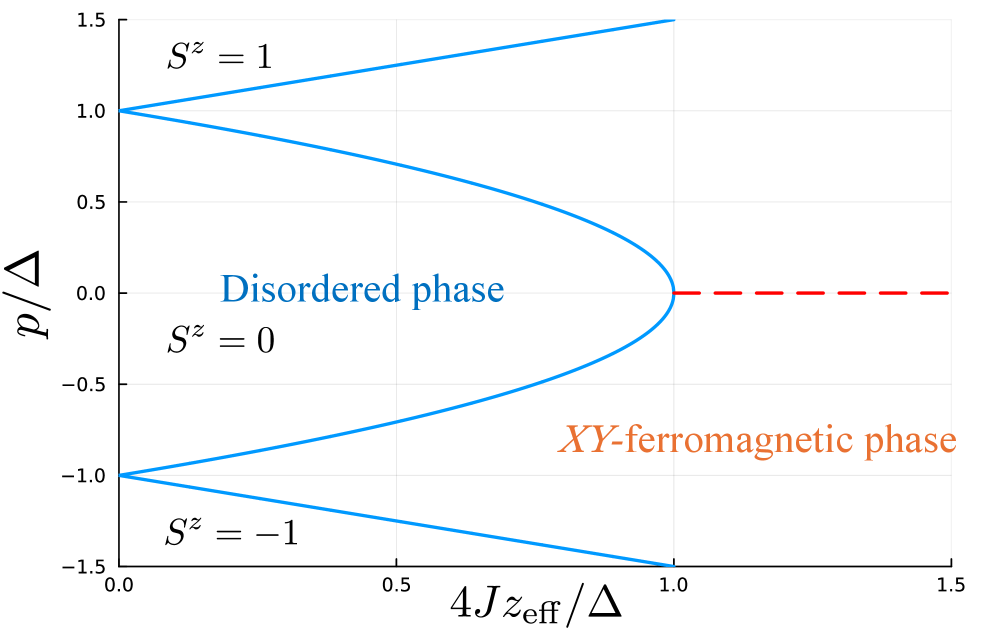
Figure 1: Ground-state phase diagram of the spin-1 $XY$ model of Eq. (1) obtained within the mean-field approximation for $\alpha>d$. The blue solid line represents the phase boundary between the XY-ferromagnetic ordered phase and the disordered phases. The red dashed line indicates the line of $\frac{p}{\Delta}=0$ in the ordered phase region.

When the spin-exchange interaction includes only the nearest-neighbor one, i.e., $\alpha\rightarrow\infty$, the previous theoretical studies have mapped out the ground-state phase diagram of the model of Eq. (1), which is equivalent to the Bose-Hubbard model in the limit of the large filling factor [22, 29, 30]. Figure 1 reviews the mean-field phase diagram in the $(\frac{4Jz_{\rm eff}}{\Delta},\frac{p}{\Delta})$-plane obtained in Refs. [30], where $z_{\rm eff}$ for this case represents the coordination number. When $\frac{Jz_{\rm eff}}{\Delta}\gg 1$ or the mean value of $S^{z}$ per site, which we call $\bar{S}^{z}$, is non-integer, the ground state forms an $XY$-ferromagnetic ordered phase, in which the $XY$ component of all the spins are aligned in a particular direction. This phase spontaneously breaks the continuous U(1) symmetry of the Hamiltonian. When $\frac{Jz_{\rm eff}}{\Delta}$ is decreased along $\frac{p}{\Delta}=0$, where $\bar{S}^{z}=0$, a continuous quantum phase transition to the disordered phase occurs at a certain critical point. The phase boundary $\left(\frac{p}{\Delta}\right)_{\rm c}$ as a function of $\frac{Jz_{\rm eff}}{\Delta}$ reads $\pm\sqrt{1-\frac{4Jz_{\rm eff}}{\Delta}}$. Introducing a dimensionless parameter $u=\frac{\Delta}{4Jz_{\mathrm{eff}}}$, the critical point $u_{\rm c}$ along $\frac{p}{\Delta}=0$ is given by $u_{\rm c}=1$ within the mean-field approximation. In this sense, $u$ measures the distance from the critical point. Notice that more precise values of $u_{\rm c}$ for $d=1$, 2, and 3 have been also computed by means of more sophisticated numerical methods [32, 33, 34]. When $\bar{S}^{z}=\pm 1$, the ground state is trivially a disordered phase and the boundary to the $XY$ ferromagnetic phase is given by $\left(\frac{p}{\Delta}\right)_{\rm c}=\pm\left(1+\frac{2Jz_{\rm eff}}{\Delta}\right)$. In the next section, we will see that in the case of the long-range interactions ($d<\alpha$), the ground-state phase diagram is identical to the case of the nearest-neighbor one with the replacement of $z_{\rm eff}$ by that for the long-range interaction.

The previous theoretical studies on the nearest-neighbor case have also shown that the system in the $XY$ ferromagnetic ordered phase for $\bar{S}^{z}=0$ possesses the Higgs and Nambu-Goldstone (NG) modes, which respectively corresponds to fluctuations of the amplitude and phase of the order parameter, as low-energy elementary excitations [22, 29, 30]. The presence of the Higgs amplitude mode can be attributed to the particle-hole symmetry at $\frac{p}{\Delta}=0$, i.e., the symmetry with respect to the replacement of $\hat{S}^{z}_{j}$ by $-\hat{S}^{z}_{j}$. The lifetime of the Higgs mode has been also evaluated to elucidate that the Higgs mode is severely damped at $d=2$ both for zero and finite temperatures due to strong effects of quantum and/or thermal fluctuations [22, 23, 24, 25, 26]. In the following sections, we will show that the long-range interaction significantly suppresses the effects of the fluctuations so that the Higgs mode can be long-lived even at $d=2$.

III Methods

In this section, we present theoretical methods for analyzing low-energy excitations in the $XY$ ferromagnetic phase of the model (1) near the transition to the disordered phase, namely, the NG and Higgs modes. Specifically, we apply the mean-field and quantum-field-theoretical approaches, which have been used for the case of the nearest-neighbor interaction in Ref. [29, 30], to our system with the long-range interaction.

III.1 Mean-field approximation

We approximate the quantum many-body state of the system as the following variational state that takes a form of the simple product state [22],

$$|\Omega\rangle= \bigotimes_{j}\left\{\cos\left(\frac{\theta_{j}}{2}\right)|0\rangle_{j}+e^{i\eta_{j}}\sin\left(\frac{\theta_{j}}{2}\right)\right.$$

$$\left.\times\left[e^{i\varphi_{j}}\sin\left(\frac{\chi_{j}}{2}\right)|1\rangle_{j}+e^{-i\varphi_{j}}\cos\left(\frac{\chi_{j}}{2}\right)|-1\rangle_{j}\right]\right\},$$ (2)

where $\theta_{j}\in[0,\pi]$, $\eta_{j}\in[-\pi/2,\pi/2]$, $\varphi_{j}\in[0,2\pi]$, and $\chi_{j}\in[0,\pi]$ are the variational parameters specifying the state. While the variational parameters in general depends on $j$, those for the $XY$ ferromagnetic ordered state and the disordered states, which are candidates for the ground state, are homogeneous so that we henceforth set $(\theta_{j},\eta_{j},\varphi_{j},\chi_{j})=(\theta,\eta,\varphi,\chi)$. The variational parameters for the ground states are determined in a way such that the mean-field energy per site

$$\!\!\!\!\!\!\!\!\!\!E^{\mathrm{MF}}=\frac{1}{M}\langle\Omega|\hat{H}|\Omega\rangle=\left(\Delta+p\cos\chi\right)\sin^{2}\left(\frac{\theta}{2}\right)$$

$$\,\,\,\,\,\,\,\,\,\,\,\,\,\,\,\,\,\,\,\,\,\,\,\,\,\,\,\,\,\,\,\,\,\,\,\,\,\,\,\,\,\,\,\,-\frac{Jz_{\mathrm{eff}}}{2}\sin^{2}\theta\left(1+\sin\chi\cos(2\eta)\right),$$ (3)

is minimized, where $M$ is the total number of sites. In the case of the long-range interaction, the effective coordination number $z_{\rm eff}$ constitutes the summation of all the interaction terms as

$$z_{\mathrm{eff}}=\sum_{l\neq 0}\frac{J_{0,l}}{J},$$ (4)

where ${\bf r}_{l}=0$ at $l=0$. For the specific case of $\alpha=3$ and $d=2$, which is the most relevant to Rydberg-atom experiments, its numerical value is $9.032$ [35].

The variational state can represent both of the $XY$ ferromagnetic ordered phase and the disordered phases. To see this, we explicitly express the $XY$ ferromagnetic order parameter $\Psi=\langle\Omega|\hat{S}^{-}_{j}|\Omega\rangle$ and the mean value of $\hat{S}_{j}^{z}$ per site as

$$\Psi=\frac{1}{\sqrt{2}}e^{i\varphi}\sin\theta\left(e^{i\eta}\sin\left(\frac{\chi}{2}\right)+e^{-i\eta}\cos\left(\frac{\chi}{2}\right)\right),$$ (5)

$$\bar{S}^{z}=\langle\Omega|\hat{S}^{z}_{j}|\Omega\rangle=-\cos\chi\sin^{2}\left(\frac{\theta}{2}\right).$$ (6)

Equations (5) and (6) imply that the disordered states, where $\Psi=0$, with $\bar{S}^{z}=1$ and $-1$ correspond to the states with $(\theta,\chi)=(\pi,\pi)$ and $(\pi,0)$ while the other parameters are not determined. That with $\bar{S}^{z}=0$ corresponds to $\theta=0$. The variational state with $\theta\neq 0$ represents the $XY$ ferromagnetic phase. In this phase, one can easily see from Eq. (3) that $\eta=0$ and $\varphi$ can be chosen arbitrarily. Without loss of generality, we choose $\varphi=0$, which means that the U(1) symmetry of the model (1) is spontaneously broken in this phase. Moreover, when $\frac{p}{\Delta}=0$, $\chi=\frac{\pi}{2}$ is satisfied.

From the Ginzburg-Landau expansion of $E^{\mathrm{MF}}$ of the ground state with respect to the order parameter $\Psi$, one can determine the boundaries between the XY ferromagnetic ordered phase to the disordered phases. The phase boundaries are identical to the case of the nearest-neighbor interaction, which was discussed in the previous section, by extending the coordination number to the effective one $z_{\rm eff}$. Recall that the ground-state phase diagram is shown in Fig. 1.

III.2 Schwinger-boson representation of the spin-1 operators

The Hamiltonian of Eq. (1) can be represented using three Schwinger bosons [22, 29, 36]:

$$|\mu\rangle_{j}=\hat{t}^{\dagger}_{\mu,j}|\mathrm{vac}\rangle_{j},~\mathrm{for}~\mu=-1,0,1,$$

where $\ket{\mathrm{vac}}$ is the vacuum of the new bosons. The commutation relations are $[\hat{t}_{\mu,j},\hat{t}^{\dagger}_{\mu^{\prime},j^{\prime}}]=\delta_{\mu,\mu^{\prime}}\delta_{j,j^{\prime}}$ and $[\hat{t}_{\mu,j},\hat{t}_{\mu^{\prime},j^{\prime}}]=[\hat{t}^{\dagger}_{\mu,j},\hat{t}^{\dagger}_{\mu^{\prime},j^{\prime}}]=0$. In order to eliminate the unphysical states such as $\hat{t}^{\dagger}_{1,j}\hat{t}^{\dagger}_{0,j}|\mathrm{vac}\rangle$, we assume that these operators obey a constraint,

$$\sum_{\mu=-1}^{1}\hat{t}^{\dagger}_{\mu,j}\hat{t}_{\mu,j}=1,$$ (7)

where $1$ on the right-hand side is the identity operator.

The spin operators are represented as

$$\hat{S}^{+}_{j} =\sqrt{2}(\hat{t}^{\dagger}_{1,j}\hat{t}_{0,j}+\hat{t}^{\dagger}_{0,j}\hat{t}_{-1,j}),$$

$$\hat{S}^{z}_{j} =\hat{t}^{\dagger}_{1,j}\hat{t}_{1,j}-\hat{t}^{\dagger}_{-1,j}\hat{t}_{-1,j}$$

$$(\hat{S}^{z}_{j})^{2} =\hat{t}^{\dagger}_{1,j}\hat{t}_{1,j}+\hat{t}^{\dagger}_{-1,j}\hat{t}_{-1,j}.$$

One can check that with this representation they satisfy the SU(2) commutation relations $[\hat{S}^{+}_{j},\hat{S}^{-}_{l}]=2\hat{S}^{z}_{j}\delta_{j,l}$ and $[\hat{S}^{z}_{j},\hat{S}^{\pm}_{l}]=\pm\hat{S}^{\pm}_{j}\delta_{j,l}$.

Let us introduce a canonical transformation in the following manner [22],

$$\hat{b}^{\dagger}_{0,j} =c_{1}\hat{t}^{\dagger}_{0,j}+\frac{1}{\sqrt{2}}s_{1}\left[\hat{t}^{\dagger}_{1,j}+\hat{t}^{\dagger}_{-1,j}\right],$$

$$\hat{b}^{\dagger}_{\mathrm{A},j} =s_{1}\hat{t}^{\dagger}_{0,j}-\frac{1}{\sqrt{2}}c_{1}\left[\hat{t}^{\dagger}_{1,j}+\hat{t}^{\dagger}_{-1,j}\right],$$ (8)

$$\hat{b}^{\dagger}_{\Phi,j} =\frac{1}{\sqrt{2}}\left[\hat{t}^{\dagger}_{1,j}-\hat{t}^{\dagger}_{-1,j}\right],$$

where the coefficients are $s_{1}=\sin\left(\frac{\theta_{\mathrm{gs}}}{2}\right)$ and $c_{1}=\cos\left(\frac{\theta_{\mathrm{gs}}}{2}\right)$. Moreover, $\theta_{\mathrm{gs}}$ denotes the value of the variational parameter $\theta$ for the ground state, $\hat{b}^{\dagger}_{\mathrm{0},j}$ the creation operator of the mean-field ground state, and $\hat{b}^{\dagger}_{\mathrm{A},j}$ ($\hat{b}^{\dagger}_{\Phi,j}$) the creation operator for the amplitude (phase) fluctuation of the order parameter. These new operators fulfill the same bosonic commutation relations as $\hat{t}_{m,j}$. In addition, the transformation retains the constraint (7) so that

$$\sum_{m\in\{0,\mathrm{A},\Phi\}}\hat{b}^{\dagger}_{m,j}\hat{b}_{m,j}=1.$$ (9)

Substituting the canonical transformation (8) into the Hamiltonian of Eq. (1), one can express the Hamiltonian in terms of $\hat{b}_{m,j}$.

III.3 Holstein-Primakoff expansion

In this subsection, assuming that quantum and thermal fluctuations from the $XY$ ferromagnetic ground state are weak, we expand the Hamiltonian with respect to $\hat{b}_{{\rm A},j}$ and $\hat{b}_{\Phi,j}$ in order to understand the low-energy physics of the system in the framework of the quasi-particle picture, in which the Higgs and NG modes play crucial roles. Specifically, we use the Holstein-Primakoff expansion [37].

$$\hat{b}^{\dagger}_{m,j}\hat{b}_{0,j} =\hat{b}^{\dagger}_{m,j}\sqrt{1-\hat{b}^{\dagger}_{\mathrm{A},j}\hat{b}_{\mathrm{A},j}-\hat{b}^{\dagger}_{\Phi,j}\hat{b}_{\Phi,j}}$$ (10)

$$\simeq\hat{b}^{\dagger}_{m,j}-\frac{1}{2}\hat{b}^{\dagger}_{m,j}\hat{b}^{\dagger}_{\mathrm{A},j}\hat{b}_{\mathrm{A},j}-\frac{1}{2}\hat{b}^{\dagger}_{m,j}\hat{b}^{\dagger}_{\Phi,j}\hat{b}_{\Phi,j}+\cdots.$$

Eliminating $\hat{b}^{\dagger}_{0,j}$ and $\hat{b}_{0,j}$ in the Hamiltonian by using the constraint (9), and substituting the Holstein-Primakoff expansion (10) into the Hamiltonian, we obtain the following series,

$$\hat{H}\simeq\hat{H}^{(0)}+\hat{H}^{(1)}+\hat{H}^{(2)}+\hat{H}^{(3)}+\cdots,$$ (11)

where $\hat{H}^{(i)}$ (for $i=0,1,2,3,\ldots$) represents the $i$th order perturbation term with respect to $\hat{b}_{m,j}$. The expansion (11) is stopped at $i=3$. We keep cubic terms in the expansion to capture the Beliaev damping process, where a Higgs mode decays into two NG modes. In the case of finite temperatures, the above truncation is valid only at $d\geq 2$, where the long-range $XY$ ferromagnetic order is present in the thermal equilibrium state. Notice that when the interaction is long-ranged as $d<\alpha<d+2$, the long-range order holds even at $d=2$, i.e., the celebrated Mermin-Wagner theorem, which prohibits the long-range order associated with a spontaneously breaking of a continuous symmetry, is evaded [27, 28].

Let us explain more details of the terms $\hat{H}^{(0)}$, $\hat{H}^{(1)}$, $\hat{H}^{(2)}$, and $\hat{H}^{(3)}$, respectively. The zeroth-order term $\hat{H}^{(0)}$ is equal to the ground state energy with no fluctuation,

$$\hat{H}^{(0)}=ME^{\mathrm{MF}}_{\rm gs},$$ (12)

where $E^{\mathrm{MF}}_{\rm gs}$ is the mean-field energy per site of the $XY$ ferromagnetic ground state (See Sec. III.2). The linear term $\hat{H}^{(1)}$ is given by

$$\hat{H}^{(1)}=A_{1}(\hat{b}^{\dagger}_{\mathrm{A},\mathbf{0}}+\hat{b}_{\mathrm{A},\mathbf{0}}),$$ (13)

where we have introduced the Fourier transformation of $\hat{b}^{\dagger}_{\mathrm{A},j}$ and $\hat{b}^{\dagger}_{\Phi,j}$,

$$\hat{b}^{\dagger}_{m,j}=\frac{1}{\sqrt{M}}\sum_{\mathbf{k}\in\Lambda_{0}}\hat{b}^{\dagger}_{m,\mathbf{k}}e^{-i\mathbf{k}\cdot\mathbf{r}_{j}},~m\in\left\{\mathrm{A},\Phi\right\}.$$ (14)

The notation $\sum_{\mathbf{k}\in\Lambda_{0}}$ means that the momentum $\mathbf{k}$ runs over the first Brillouin zone $\Lambda_{0}\equiv[-\pi,\pi]^{d}$. For the mean-field ground state, we can easily verify that $\hat{H}^{(1)}=0$. The quadratic term $\hat{H}^{(2)}$ can be written as

$$\hat{H}^{(2)} =\sum_{\mathbf{k}}B_{1}\hat{b}^{\dagger}_{\mathrm{A},\mathbf{k}}\hat{b}_{\mathrm{A},\mathbf{k}}$$

$$\!\!\!\!\!\!\!\!\!\!\!+\!\sum_{\mathbf{k}}B_{2}(\hat{b}^{\dagger}_{\mathrm{A},\mathbf{k}}\hat{b}^{\dagger}_{\mathrm{A},-\mathbf{k}}+\hat{b}_{\mathrm{A},\mathbf{k}}\hat{b}^{\dagger}_{\mathrm{A},\mathbf{k}}+\hat{b}^{\dagger}_{\mathrm{A},\mathbf{k}}\hat{b}_{\mathrm{A},\mathbf{k}}+\hat{b}_{\mathrm{A},\mathbf{k}}\hat{b}_{\mathrm{A},-\mathbf{k}})$$

$$\!\!\!\!\!\!\!\!\!\!\!+\sum_{\mathbf{k}}C_{1}\hat{b}^{\dagger}_{\Phi,\mathbf{k}}\hat{b}_{\Phi,\mathbf{k}}$$

$$\!\!\!\!\!\!\!\!\!\!\!+\!\sum_{\mathbf{k}}C_{2}(\hat{b}^{\dagger}_{\Phi,\mathbf{k}}\hat{b}^{\dagger}_{\Phi,-\mathbf{k}}+\hat{b}_{\Phi,\mathbf{k}}\hat{b}^{\dagger}_{\Phi,\mathbf{k}}+\hat{b}^{\dagger}_{\Phi,\mathbf{k}}\hat{b}_{\Phi,\mathbf{k}}+\hat{b}_{\Phi,\mathbf{k}}\hat{b}_{\Phi,-\mathbf{k}}).$$ (15)

The cubic term $\hat{H}^{(3)}$, which describes the interaction between the Higgs and NG modes, can be expressed as

$$\hat{H}^{(3)} =\sum_{\mathbf{k}_{1},\mathbf{k}_{2},\mathbf{k}_{3}}D_{1}(\hat{b}^{\dagger}_{\Phi,\mathbf{k}_{1}}\hat{b}_{\Phi,\mathbf{k}_{2}}\hat{b}_{\mathrm{A},\mathbf{k}_{3}}+\mathrm{H.c.})$$

$$+\sum_{\mathbf{k}_{1},\mathbf{k}_{2},\mathbf{k}_{3}}D_{2}(\hat{b}^{\dagger}_{\mathrm{A},\mathbf{k}_{1}}\hat{b}_{\mathrm{A},\mathbf{k}_{2}}\hat{b}_{\mathrm{A},\mathbf{k}_{3}}+\mathrm{H.c.})$$

$$\!\!\!\!\!\!\!\!\!\!\!+\sum_{\mathbf{k}_{1},\mathbf{k}_{2},\mathbf{k}_{3}}D_{3}(\hat{b}^{\dagger}_{\mathrm{A},\mathbf{k}_{1}}\hat{b}_{\Phi,\mathbf{k}_{2}}\hat{b}_{\Phi,\mathbf{k}_{3}}-\hat{b}^{\dagger}_{\Phi,\mathbf{k}_{1}}\hat{b}_{\mathrm{A},\mathbf{k}_{2}}\hat{b}_{\Phi,\mathbf{k}_{3}}+\mathrm{H.c.}).$$ (16)

For the explicit expressions of the coefficients $A_{1}$, $B_{1}$, $B_{2}$, $C_{1}$, $C_{2}$, $D_{1}$, $D_{2}$, and $D_{3}$, see Appendix A.

III.4 Bogoliubov transformation

In Sec. III.3, we have obtained the series of the Hamiltonian in terms of $\hat{b}_{\mathrm{A},j}$ and $\hat{b}_{\Phi,j}$. As we have seen in Sec. III.3, $\hat{H}^{(2)}$ has no mixing term between branches labeled by $\mathrm{A}$ and $\Phi$. Hence, we can diagonalize $\hat{H}^{(2)}$ by performing the Bogoliubov transformation independently in each branch as

$$\hat{b}_{m,\mathbf{k}}=u_{m,\mathbf{k}}\hat{\eta}_{m,\mathbf{k}}+v^{\ast}_{m,-\mathbf{k}}\hat{\eta}^{\dagger}_{m,-\mathbf{k}},$$ (17)

where the operator $\hat{\eta}_{m,{\bf k}}$ obeys the bosonic commutation relations $[\hat{\eta}_{m,\mathbf{k}},\hat{\eta}^{\dagger}_{n,-\mathbf{k}^{\prime}}]=\delta_{m,n}\delta_{\mathbf{k},\mathbf{k}^{\prime}}$ and $[\hat{\eta}_{m,\mathbf{k}},\hat{\eta}_{n,-\mathbf{k}^{\prime}}]=[\hat{\eta}^{\dagger}_{m,\mathbf{k}},\hat{\eta}^{\dagger}_{n,-\mathbf{k}^{\prime}}]=0$.

Let us assume that the coefficients are real and have a symmetry under a sign change of the momentum $\mathbf{k}\to-\mathbf{k}$. Under this assumption, one can obtain the coefficients of the transformation,

$$u_{{\rm A},\mathbf{k}} =\sqrt{\frac{2-u^{2}\gamma_{\mathbf{k}}}{4\sqrt{1-u^{2}\gamma_{\mathbf{k}}}}+\frac{1}{2}},$$ (18)

$$v_{{\rm A},\mathbf{k}} =\mathrm{sgn}(\gamma_{\mathbf{k}})\sqrt{\frac{2-u^{2}\gamma_{\mathbf{k}}}{4\sqrt{1-u^{2}\gamma_{\mathbf{k}}}}-\frac{1}{2}},$$ (19)

$$u_{\Phi,\mathbf{k}} =\sqrt{\frac{2-\gamma_{\mathbf{k}}}{4\sqrt{1-\gamma_{\mathbf{k}}}}+\frac{1}{2}},$$ (20)

$$v_{\Phi,\mathbf{k}} =-\mathrm{sgn}(\gamma_{\mathbf{k}})\sqrt{\frac{2-\gamma_{\mathbf{k}}}{4\sqrt{1-\gamma_{\mathbf{k}}}}-\frac{1}{2}},$$ (21)

where

$$\gamma_{\mathbf{k}}=\frac{1}{z_{\mathrm{eff}}}\sum_{j\neq 0}\frac{e^{i\mathbf{k}\cdot\mathbf{r}_{j}}}{|\mathbf{r}_{0,j}|^{\alpha}}.$$ (22)

Notice that $-Jz_{\rm eff}\gamma_{\bf k}$ forms the band structure of a single particle in the hyper-cubic lattice. After this transformation, the Hamiltonian of Eq. (11) reads

$$\hat{H}\simeq\sum_{m\in\{\mathrm{A},\Phi\}}\sum_{\mathbf{k}}\mathcal{E}_{m,\mathbf{k}}\hat{\eta}^{\dagger}_{m,\mathbf{k}}\hat{\eta}_{m,\mathbf{k}}+\hat{H}^{(3)}(\hat{\eta}^{\dagger}_{m,\mathbf{k}},\hat{\eta}_{m,\mathbf{k}}).$$ (23)

The dispersions of the Higgs and NG modes are given by

$$\mathcal{E}_{\mathrm{A},\mathbf{k}} =4Jz_{\mathrm{eff}}\sqrt{1-u^{2}\gamma_{\mathbf{k}}},$$ (24)

$$\mathcal{E}_{\Phi,\mathbf{k}} =2Jz_{\mathrm{eff}}(1+u)\sqrt{1-\gamma_{\mathbf{k}}}.$$ (25)

The former dispersion, corresponding to the Higgs mode, has an energy gap

$$\Delta_{\mathrm{h}}=4Jz_{\mathrm{eff}}\sqrt{1-u^{2}}$$ (26)

at $\mathbf{k}=\mathbf{0}$, whereas the latter dispersion, corresponding to the NG mode, is gapless. The energy gap $\Delta_{\mathrm{h}}$ closes at the critical point $u=u_{\rm c}=1$.

III.5 Finite-temperature Green’s functions

To evaluate the Beliaev damping rate of the Higgs mode, we employ the finite-temperature Green’s-function formalism [38, 39, 40]. The single-particle Green’s function of the Higgs mode is defined as

$$\mathcal{G}_{\mathrm{A},\mathbf{k}}(i\omega_{n})\equiv\frac{\int\mathcal{D}(\eta,\bar{\eta})\eta_{\mathrm{A},\mathbf{k}}(i\omega_{n})\bar{\eta}_{\mathrm{A},\mathbf{k}}(i\omega_{n})\exp(-\mathcal{S})}{\int\mathcal{D}(\eta,\bar{\eta})\exp(-\mathcal{S})},$$ (27)

where $\omega_{n}=\frac{2\pi n}{\beta}\quad(n\in\mathbb{N})$ is the Matsubara frequency [38, 39, 40], $\beta=T^{-1}$ is the inverse temperature, $\eta_{\mathrm{A},\mathbf{k}}(i\omega_{n})$ and its conjugate $\bar{\eta}_{\mathrm{A},\mathbf{k}}(i\omega_{n})=(\eta_{\mathrm{A},\mathbf{k}}(i\omega_{n}))^{\ast}$ are complex-valued field variables at $(\omega_{n},\mathbf{k})$, and $\mathcal{D}(\eta,\bar{\eta})$ is a measure of the integrations. The action

$$\mathcal{S}=\mathcal{S}^{(2)}+\mathcal{S}^{(3)}+\tilde{\mathcal{S}}^{(3)}$$ (28)

is derived from Eq. (23). The quadratic action $\mathcal{S}^{(2)}$ is given by

$$\mathcal{S}^{(2)}\!=\!\sum_{m\in\{\mathrm{A},\Phi\}}\!\sum_{\mathbf{k}}\sum_{n}(-i\omega_{n}+\mathcal{E}_{m,\mathbf{k}})\bar{\eta}_{m,\mathbf{k}}(i\omega_{n})\eta_{m,\mathbf{k}}(i\omega_{n}).$$ (29)

$\mathcal{S}^{(3)}$ stems from a part of the cubic terms $\hat{H}^{(3)}$, which includes only the $\hat{b}^{\dagger}_{\mathrm{A},\mathbf{k}_{1}}\hat{b}_{\Phi,\mathbf{k}_{2}}\hat{b}_{\Phi,\mathbf{k}_{3}}$ term and its Hermitian conjugate, and is given by

$$\mathcal{S}^{(3)}=\frac{1}{2\sqrt{\beta}}\sum_{n_{1},n_{2},n_{3}}\sum_{\mathbf{k}_{1},\mathbf{k}_{2},\mathbf{k}_{3}}\delta_{n_{1},n_{2}+n_{3}}\mathcal{M}_{\mathbf{k}_{1},\mathbf{k}_{2},\mathbf{k}_{3}}$$

$$\times\left(\eta_{\mathrm{A},\mathbf{k}_{1}}(i\omega_{n_{1}})\bar{\eta}_{\Phi,\mathbf{k}_{2}}(i\omega_{n_{2}})\bar{\eta}_{\Phi,\mathbf{k}_{3}}(i\omega_{n_{3}})+\mathrm{c.c.}\right).$$ (30)

For the explicit form of $\mathcal{M}_{\mathbf{k}_{1},\mathbf{k}_{2},\mathbf{k}_{3}}$, see Appendix A. $\tilde{\mathcal{S}}^{(3)}$ contains the other part of the cubic terms. We separately describe $\mathcal{S}^{(3)}$ and $\tilde{\mathcal{S}}^{(3)}$ because the former contributes to the damping of the Higgs mode with ${\bf k}={\bf 0}$ owing to the energy and momentum conservation laws but the latter does not.

The single particle Green’s function $\mathcal{G}_{\mathrm{A},\mathbf{k}}(i\omega_{n})$ fulfills the Dyson’s equations [39, 40]:

$$\mathcal{G}_{\mathrm{A},\mathbf{k}}(i\omega_{n})=\mathcal{G}^{(0)}_{\mathrm{A},\mathbf{k}}(i\omega_{n})+\mathcal{G}^{(0)}_{\mathrm{A},\mathbf{k}}(i\omega_{n})\tilde{\Sigma}_{\mathrm{A},{\bf k}}(i\omega_{n})\mathcal{G}_{\mathrm{A},\mathbf{k}}(i\omega_{n}),$$ (31)

where $\tilde{\Sigma}_{\mathrm{A},{\bf k}}(i\omega_{n})$ is the self-energy function of the Higgs mode and $\mathcal{G}^{(0)}_{\mathrm{A},\mathbf{k}}(i\omega_{n})=1/(i\omega_{n}-\mathcal{E}_{\mathrm{A},\mathbf{k}})$ is the free propagator of the Higgs mode.

We evaluate the lowest-order (one-loop) self-energy diagram using the perturbative Green’s-function formalism introduced in Sec. III.5. Hereafter, we focus on the Higgs mode with zero momentum $\mathbf{k}={\bf 0}$ because such an excitation can be created relatively easily in experiments of Rydberg-atom arrays by a global control of the parameter $\Delta$.

At the second order, the self-energy of the Higgs mode with $\mathbf{k}={\bf 0}$ is given by

$$\tilde{\Sigma}_{\mathrm{A},{\bf k}={\bf 0}}(i\omega_{n})=\frac{1}{2}\sum_{\mathbf{k}\in\Lambda_{0}}|\mathcal{M}_{\mathbf{0},\mathbf{k},-\mathbf{k}}|^{2}\frac{1+2n_{\mathrm{B}}\left(\mathcal{E}_{\Phi,\mathbf{k}}\right)}{i\omega_{n}-2\mathcal{E}_{\Phi,\mathbf{k}}},$$ (32)

where $n_{\mathrm{B}}(x)=(e^{\beta x}-1)^{-1}$ is the Bose distribution function.

In order to obtain the damping rate of the Higgs mode $\Gamma_{\mathrm{A},\mathbf{k}=\mathbf{0}}$, we make an analytic continuation, $\omega_{n}\rightarrow\omega+i\epsilon$, that converts the self-energy for the Matsubara Green’s function to the one for the retarded Green’s function and take the imaginary part of the latter as

$$\Gamma_{\mathrm{A},\mathbf{k}=\mathbf{0}} =\mathrm{Im}\tilde{\Sigma}_{\mathrm{A},{\bf k}={\bf 0}}(i\omega_{n})|_{i\omega_{n}\to\omega+i\epsilon}$$

$$\!\!\!\!\!\!\!\!=\frac{\pi}{2}\sum_{\mathbf{k}\in\Lambda_{0}}|\mathcal{M}_{\mathbf{0},\mathbf{k},-\mathbf{k}}|^{2}(1+2n_{\mathrm{B}}[\mathcal{E}_{\Phi,\mathbf{k}}])\delta(\mathcal{E}_{\mathrm{A},\mathbf{0}}-2\mathcal{E}_{\Phi,\mathbf{k}}).$$ (33)

Equation (33) describes a Beliaev damping process, where one Higgs mode with zero momentum collapses into two NG modes with opposite momenta $\mathbf{k}$ and $-\mathbf{k}$ with satisfying the on-shell energy-momentum conservation of $\mathcal{E}_{\mathrm{A},\mathbf{0}}-2\mathcal{E}_{\Phi,\mathbf{k}}$.

IV Results

In this section, we discuss properties of the NG and Higgs modes with the focus on their low-energy behavior.

IV.1 Excitation spectra

When $d<\alpha<d+2$, $\gamma_{\mathbf{k}}$ at small $|{\bf k}|$ can be expanded with respect to $|{\bf k}|$ as

$$\gamma_{\mathbf{k}}\simeq 1-A|\mathbf{k}|^{\alpha-d},$$ (34)

where $A$ is a coefficient that depends on $\alpha$ and $d$ [41, 42, 43]. For the specific case of $\alpha=3$ and $d=2$, $A$ can be readily evaluated using Ewald summation [44] as $A=\frac{2\pi}{z_{\mathrm{eff}}}$. Substituting Eq. (34) into Eqs. (24) and (25), the dispersion relations of the Higgs and NG modes at small $|{\bf k}|$ are approximated as

$$\mathcal{E}_{\mathrm{A},\mathbf{k}} \simeq\sqrt{\Delta_{\mathrm{h}}^{2}+g_{\mathrm{h}}^{2}|\mathbf{k}|^{\alpha-d}}\simeq\Delta_{\rm h}+\frac{g_{\rm h}^{2}}{2\Delta_{\rm h}}|\mathbf{k}|^{\alpha-d},$$ (35)

$$\mathcal{E}_{\Phi,\mathbf{k}} \simeq g_{\mathrm{ng}}|\mathbf{k}|^{\frac{\alpha-d}{2}},$$ (36)

where

$$g_{\mathrm{h}} = 4Jz_{\rm eff}u\sqrt{A},$$ (37)

$$g_{\mathrm{ng}} = 2Jz_{\rm eff}(1+u)\sqrt{A}.$$ (38)

Since in the case of the nearest-neighbor interaction $(\mathcal{E}_{\mathrm{A},\mathbf{k}}-\Delta_{\rm h})\propto|{\bf k}|^{2}$ and $\mathcal{E}_{\Phi,\mathbf{k}}\propto|{\bf k}|$ [22, 29, 30], Eqs. (35) and (36) mean that the long-range nature of the spin-exchange interactions significantly modifies the dispersion relations. In the limit of $\alpha\rightarrow d+2$, the qualitative behavior of the dispersion relations at small $|{\bf k}|$ agrees with that for the nearest-neighbor interaction.

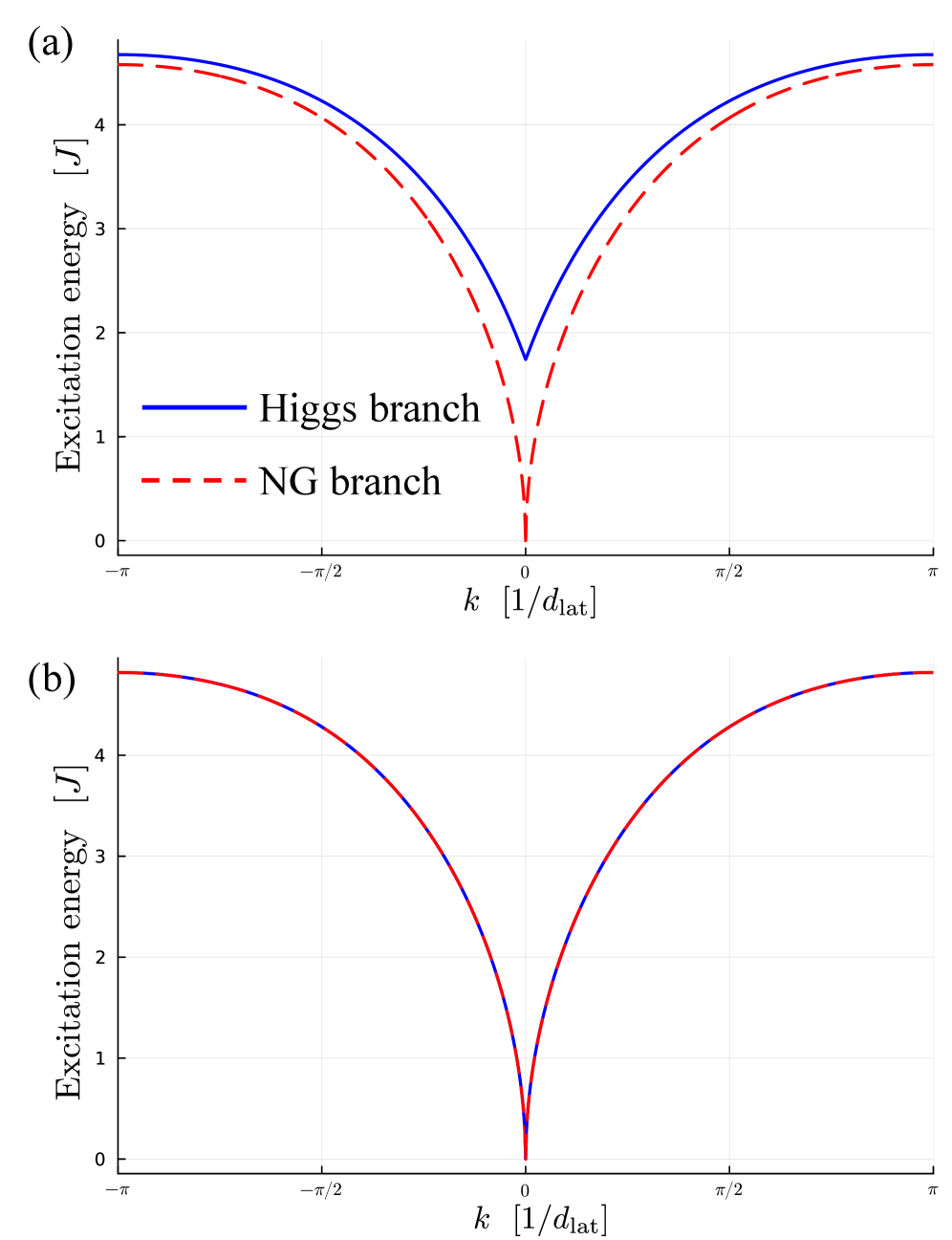
Figure 2: Dispersion relations of the Higgs (blue solid line) and NG (red dashed line) modes, which are expressed in Eqs. (24) and (25), for $d=2$, $\alpha=3$, and ${\bf k}=(k,0)$, where $u=0.9(<u_{\rm c})$ (a) and $u=u_{\rm c}$ (b).

In Fig. 2, we show the dispersion relations $\mathcal{E}_{\mathrm{A},\mathbf{k}}$ and $\mathcal{E}_{\Phi,\mathbf{k}}$ of Eqs. (24) and (25) for $\alpha=3$ and $d=2$ by setting ${\bf k}=(k,0)$. When $u=0.9$ (Fig. 2(a)), the Higgs mode exibits a gapped and linear dispersion, while the NG mode exhibits a gapless square root dispersion at small $|{\bf k}|$. As shown in Fig. 2(b), at the critical point $u=1$, the gap of the Higgs mode vanishes such that the dispersion of the Higgs mode coincides with that of the NG mode. In Fig. 3, we show the gap of the Higgs mode $\Delta_{\rm h}$ as a function of $u$. There we see that the Higgs gap obeys the critical scaling behavior $\Delta_{\mathrm{h}}\sim|u-u_{\mathrm{c}}|^{\frac{1}{2}}$. While this gap closing also occurs in the case of the nearest-neighbor interactions, the critical exponent deviates from the mean-field value $\frac{1}{2}$ [24].

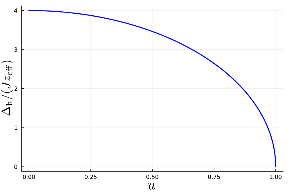
Figure 3: Higgs gap $\Delta_{\rm h}$ as a function of $u$, whose analytical expression is given in Eq. (26).

IV.2 Beliaev damping rate

We discuss the Beliaev damping of the Higgs mode at finite temperatures by obtaining an approximate analytical expression of the damping rate $\Gamma_{{\rm A},{\bf k}={\bf 0}}$. For this purpose, let us evaluate the integrals of Eq. (33) within the long-wavelength approximation, where $u_{m,\mathbf{k}}$ and $v_{m,\mathbf{k}}$ are approximated as

$$u_{\mathrm{A},\mathbf{k}}\simeq\frac{1}{\sqrt{2\bar{\Delta}_{\mathrm{h}}}}, \quad v_{\mathrm{A},\mathbf{k}}\simeq\frac{1}{\sqrt{2\bar{\Delta}_{\mathrm{h}}}},$$

$$u_{\Phi,\mathbf{k}}\simeq\sqrt{\frac{u+1}{4\bar{g}_{\mathrm{ng}}\sqrt{|\mathbf{k}|}}}, \quad v_{\Phi,\mathbf{k}}\simeq-\sqrt{\frac{u+1}{4\bar{g}_{\mathrm{ng}}\sqrt{|\mathbf{k}|}}},$$

where $\bar{\Delta}_{\mathrm{h}}=\frac{\Delta_{\mathrm{h}}}{Jz_{\mathrm{eff}}}$ and $\bar{g}_{\mathrm{ng}}=\frac{g_{\mathrm{ng}}}{Jz_{\mathrm{eff}}}$. This approximation is better justified in a closer vicinity of the critical point $u=u_{\rm c}$, where the momenta of the NG modes with energy $\frac{\Delta_{\mathrm{h}}}{2}$ contributed dominantly to the damping of the Higgs mode are smaller. Performing the integration with respect to $\mathbf{k}$ on the right hand side of Eq. (33), we obtain the simple formula,

$$\Gamma_{\mathrm{A},\mathbf{k}=\mathbf{0}}\simeq \frac{\pi Jz_{\mathrm{eff}}}{8(\alpha-d)}\frac{\Omega_{d}\sqrt{1-u^{2}}(1+u)}{(2\pi)^{d}A^{3/2}}$$

$$\times\left(\frac{\Delta_{\mathrm{h}}}{2g_{\mathrm{ng}}}\right)^{\frac{5d-3\alpha}{\alpha-d}}\coth\left(\frac{\beta\Delta_{\mathrm{h}}}{4}\right),$$ (39)

where

$$\Omega_{d}=\frac{2\pi^{\frac{d}{2}}}{\Gamma(\frac{d}{2})}$$ (40)

denotes the surface area of a unit sphere in $d$ dimensions. It is obvious from Eq. (39) that the dependence on temperature $T$ is determined by the factor $\coth\left(\frac{\beta\Delta_{\mathrm{h}}}{4}\right)$.

For the specific case of $\alpha=3$ and $d=2$, the damping rate becomes

$$\Gamma_{\mathrm{A},\mathbf{k}={\bf 0}}=\frac{Jz_{\mathrm{eff}}^{3}(1-u^{2})}{16\pi^{2}}\coth\left(\frac{\beta\Delta_{\mathrm{h}}}{4}\right).$$ (41)

For another specific case of $\alpha\to 5$ and $d=3$, which corresponds to previous works [22, 29], it is

$$\Gamma_{\mathrm{A},\mathbf{k}={\bf 0}}=\frac{3^{\frac{3}{2}}Jz_{\mathrm{eff}}(1+u)\sqrt{1-u^{2}}}{2\sqrt{2}\pi}\coth\left(\frac{\beta\Delta_{\mathrm{h}}}{4}\right).$$ (42)

The expression of Eq. (42) with the replacement of $z_{\rm eff}$ by the coordination number $z$ agrees with those in the previous works.

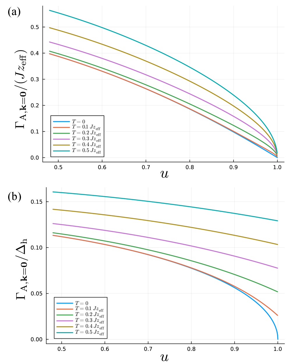
Figure 4: Beliaev damping rate of the Higgs mode as a function of $u$ for $d=2$ and $\alpha=3$, which is expressed in Eq. (41). (a) $\Gamma_{\mathrm{A},\mathbf{k}=\mathbf{0}}/(Jz_{\mathrm{eff}})$ and (b) $\Gamma_{\mathrm{A},\mathbf{k}=\mathbf{0}}/\Delta_{\mathrm{h}}$.

In Fig. 4(a), we show the damping rate $\frac{\Gamma_{{\rm A},{\bf k}={\bf 0}}}{Jz_{\rm eff}}$ as a function of $u$ for $\alpha=3$, $d=2$, and several values of the temperature. We find that the damping rate increases monotonically with the temperature for a given $u$, but it vanishes at the critical point regardless of the value of the temperature. In Fig. 4(b), we show the damping rate measured by the Higgs gap $\frac{\Gamma_{{\rm A},{\bf k}={\bf 0}}}{\Delta_{\rm h}}$ for $\alpha=3$, $d=2$, and several values of the temperature. At a finite temperature in the region of $0<T\leq 0.5Jz_{\rm eff}$, $\frac{\Gamma_{{\rm A},{\bf k}={\bf 0}}}{\Delta_{\rm h}}$ converges to a finite value, which is suffiently smaller than unity, in the limit of $u\rightarrow 1$. This fact indicates that the long-range interaction significantly suppresses the damping of the Higgs mode near the critical point so that the collective oscillation of the Higgs mode can be long-lived at sufficiently low temperatures, i.e., not over-damped at least. Notice that a similar suppression of the damping of the Higgs mode due to a kind of long-range interaction has been pointed out for a two-dimensional superconductor [45]. Nevertheless, the mechanism of the suppression is totally different from our case in the sense that there the type of long-range interaction is the density-density interaction and the ordered phase is a fermionic supercondoctor with cooper pairs.

It is worth emphasizing that in the case of the nearest-neighbor interaction, the collective oscillation of the Higgs mode at ${\bf k}={\bf 0}$ is over-damped at finite temperatures even for $d=3$ [29, 30]. We can understand this from Eq. (42). Specifically, $\frac{\Gamma_{{\rm A},{\bf k}={\bf 0}}}{\Delta_{\rm h}}$ for $\alpha\to 5$ and $d=3$ is proportional to $\frac{T}{\Delta_{\rm h}}$ near the critical point so that it diverges in the limit of $u\rightarrow 1$. By contrast, Eq. (41) implies that $\frac{\Gamma_{{\rm A},{\bf k}={\bf 0}}}{\Delta_{\rm h}}$ for $\alpha=3$ and $d=2$ is proportional to $T$ so that it converges in the limit of $u\rightarrow 1$.

We finally discuss how to create and observe the Higgs mode at ${\bf k}={\bf 0}$ in experiments of Rydberg-atom arrays described by Eq. (1). To be specific, we consider the local spin-1 states are formed by the $|41F\rangle$, $|43D\rangle$, and $|45P\rangle$ Rydberg states as in Ref. [14]. Recall that $\Delta$ can be dynamically controlled in experiments by changing the light shift of one of the three states [31]. One needs to prepare the $XY$ ferromagnetic ordered state with $\bar{S}^{z}=0$ that possesses the Higgs mode as an elementary excitation. This can be achieved as follows: i) set $\Delta$ to be much larger than $Jz_{\rm eff}$ and excite all the atoms from the ground state to $|43D\rangle$($=|S^{z}=0\rangle$) such that the system is prepared to be in the disordered state with $\bar{S}^{z}=0$ that is the ground-state for the given $\frac{\Delta}{Jz_{\rm eff}}$. ii) decrease $\Delta$ slowly down across the critical point $u=1$ and stop the decrease around $u\simeq 1$, e.g., $u=0.9$ in order to prepare the $XY$ ferromagnetic ordered state. From this state, iii) induce the oscillation of the order-parameter amplitude, i.e., the Higgs mode by suddenly quenching $\Delta$, e.g., from $0.9$ to $0.95$. For the detection of the Higgs mode, iv) measure the time evolution of the occupation probability of each local state as done in Refs. [14]. The occupation probability should oscillate with the same frequency and damping rate as those of the Higgs mode. Thus, we suggest that the Higgs mode can be created and detected through procedure i)-iv). The temporal oscillations of the order parameter have been observed for Rydberg atom arrays described by the spin-1/2 antiferromagnetic Ising model with a mixed field, whose ground-state can be the antiferromagnetic ordered phase breaking spontaneously a discrete symmetry, in a similar setting that utilizes the combination of an adiabatic preparation of the initial state and a sudden quench of a Hamiltonian parameter [46].

V Conclusion

By means of the mean-field and quantum-field-theoretical approaches, we have analytically investigated the collective excitations in the $XY$ ferromagnetic ordered phase of the spin-1 XY model with a quadratic Zeeman term and the long-range interaction that decays with distance $r$ as $\propto r^{-\alpha}$. For the specific case of $\alpha=3$ and two dimensions, which corresponds to Rydberg-atom experiments, we found that the excitation energy of the Higgs mode exhibits a linear dispersion, whereas the dispersion of the NG mode becomes proportional to the square root of the momentum. Furthermore, our analysis revealed that long-range interaction significantly suppresses the Beliaev damping of the Higgs mode near the critical point to the disordered phase. These results suggest that the Higgs mode can be detected as a long-lived oscillation of the order parameter. We proposed a specific protocol to experimentally create and probe the Higgs mode as such an oscillation.

In the present paper, we focused on the homogeneous system. However, given the high controllability of the spatial configuration of Rydberg-atom arrays, it will be interesting to explore effects of the spatial inhomogeneity on the Higgs mode, e.g., the possibility of the presence of Higgs bound states theoretically predicted for the short-range interaction [47].

Appendix A Coefficients in the effective Hamiltonian

In this appendix, we give the coefficients in each partial Hamiltonian $\hat{H}^{(i)}$ for $i=1,2,3$.

The coefficient in the $\hat{H}^{(1)}$ are given by

$$A_{1}=4Jz_{\mathrm{eff}}s_{1}c_{1}\sqrt{M}\left(c^{2}_{1}-s^{2}_{1}-u\right)=0.$$ (43)

This implies $u=c^{2}_{1}-s^{2}_{1}$, where we recall that $u=\frac{\Delta}{4Jz_{\rm eff}}$. The coefficients in the $\hat{H}^{(2)}$ are given by

$$B_{1} =4Jz_{\mathrm{eff}},$$ (44)

$$B_{2} =-Jz_{\mathrm{eff}}u^{2}\gamma_{\mathbf{k}},$$ (45)

$$C_{1} =2Jz_{\mathrm{eff}}(1+u),$$ (46)

$$C_{2} =\frac{Jz_{\mathrm{eff}}}{2}(1+u)\gamma_{\mathbf{k}}.$$ (47)

The coefficients in the $\hat{H}^{(3)}$ are given by

$$D_{1} =-\sum_{\mathbf{k}_{1},\mathbf{k}_{2},\mathbf{k}_{3}}\frac{2}{\sqrt{M}}Jz_{\mathrm{eff}}u\sqrt{1-u^{2}}\gamma_{\mathbf{k}_{3}}\delta_{\mathbf{k}_{1}+\mathbf{k}_{3},\mathbf{k}_{2}},$$ (48)

$$D_{2} =-\sum_{\mathbf{k}_{1},\mathbf{k}_{2},\mathbf{k}_{3}}\frac{4}{\sqrt{M}}Jz_{\mathrm{eff}}u\sqrt{1-u^{2}}\gamma_{\mathbf{k}_{3}}\delta_{\mathbf{k}_{1}+\mathbf{k}_{3},\mathbf{k}_{2}},$$ (49)

$$D_{3} =\sum_{\mathbf{k}_{1},\mathbf{k}_{2},\mathbf{k}_{3}}\frac{1}{\sqrt{M}}Jz_{\mathrm{eff}}\sqrt{1-u^{2}}\gamma_{\mathbf{k}_{3}}\delta_{\mathbf{k}_{1},\mathbf{k}_{2}+\mathbf{k}_{3}}.$$ (50)

The coefficient in the $\mathcal{S}^{(3)}$ are given by

$$\mathcal{M}_{\mathbf{k}_{1},\mathbf{k}_{2},\mathbf{k}_{3}}=\frac{1}{\sqrt{M}}\delta_{\mathbf{k}_{1},\mathbf{k}_{2}+\mathbf{k}_{3}}\Bigg[ -2Jz_{\mathrm{eff}}u\sqrt{1-u^{2}}\gamma_{\mathbf{k}_{1}}(u_{\mathrm{A},\mathbf{k}_{1}}+v_{\mathrm{A},\mathbf{k}_{1}})(u_{\Phi,\mathbf{k}_{2}}v_{\Phi,\mathbf{k}_{3}}+v_{\Phi,\mathbf{k}_{2}}u_{\Phi,\mathbf{k}_{3}})$$

$$+Jz_{\mathrm{eff}}\sqrt{1-u^{2}}\gamma_{\mathbf{k}_{2}}(u_{\mathrm{A},\mathbf{k}_{1}}u_{\Phi,\mathbf{k}_{3}}-v_{\mathrm{A},\mathbf{k}_{1}}v_{\Phi,\mathbf{k}_{3}})(u_{\Phi,\mathbf{k}_{2}}-v_{\Phi,\mathbf{k}_{2}})$$

$$+Jz_{\mathrm{eff}}\sqrt{1-u^{2}}\gamma_{\mathbf{k}_{3}}(u_{\mathrm{A},\mathbf{k}_{1}}u_{\Phi,\mathbf{k}_{2}}-v_{\mathrm{A},\mathbf{k}_{1}}v_{\Phi,\mathbf{k}_{2}})(u_{\Phi,\mathbf{k}_{3}}-v_{\Phi,\mathbf{k}_{3}})\Bigg].$$ (51)

References

- [1] N. Defenu, T. Donner, T. Macri, G. Pagano, S. Ruffo, and A. Trombettoni, Rev. Mod. Phys. 95, 035002 (2023).
- [2] A. Browaeys and T. Lahaye, Nat. Phys. 16, 132 (2020).
- [3] M. Morgado, and S. Whitlock, AVS Quantum Sci. 3, 023501 (2021).
- [4] T. Lahaye, C. Menotti, L. Santos, M. Lewenstein, and T. Pfau, Rep. Prog. Phys. 72, 126401 (2009).
- [5] L. Chomaz, I. Ferrier-Barbut, F. Ferlaino, B. Laburthe-Tolra, B. L. Lev, and T. Pfau, Rep. Prog. Phys. 86, 026401 (2022).
- [6] R. Blatt and C. F. Roos, Nat. Phys. 8, 277 (2012).
- [7] C. Monroe, W. C. Campbell, L.-M. Duan, Z.-X. Gong, A. V. Gorshkov, P. W. Hess, R. Islam, K. Kim, N. M. Linke, G. Pagano, P. Richerme, C. Senko, and N. Y. Yao, Rev. Mod. Phys. 93, 025001 (2021).
- [8] H. Labuhn, D. Barredo, S. Ravets, S. de Léséleuc, T. Macrì, T. Lahaye, and A. Browaeys, Nature 534, 667-670 (2016).
- [9] H. Bernien, S. Schwartz, A. Keesling, H. Levine, A. Omran, H. Pichler, S. Choi, A. S. Zibrov, M. Endres, M. Greiner, V. Vuletić, and M. D. Lukin, Nature 551, 579-584 (2017).
- [10] P. Scholl, M. Schuler, H. J. Williams, A. A. Eberharter, D. Barredo, K. N. Schymik, V. Lienhard, L. P. Henry, T. C. Lang, T. Lahaye, A. M. Läuchli, and A. Browaeys, Nature 595 , 233-238 (2021).
- [11] S. de Léséleuc, V. Lienhard, P. Scholl, D. Barredo, S. Weber, N. Lang, H. P. Büchler, T. Lahaye, A. Browaeys, Science 365, 775-780 (2019).
- [12] C. Chen, G. Bornet, M. Bintz, G. Emperauger, L. Leclerc, V. S. Liu, P. Scholl, D. Barredo, J. Hauschild, S. Chatterjee, M. Schuler, A. M. Läuchli, M. P. Zaletel, T. Lahaye, N. Y. Yao, and A. Browaeys, Nature 616, 691-695 (2023).
- [13] C. Chen, G. Emperauger, G. Bornet, F. Caleca, B. Gély, M. Bintz, S. Catterjee, V. Liu, D. Barredo, N. Y. Yao, T. Lahaye, F. Mezzacapo, T. Roscilde, and A. Browaeys, Science 389, 483-487 (2025).
- [14] Y. Chew, T. Tomita, T. P. Mahesh, S. Sugawa, S. de Léséleuc, and K. Ohmori, Nat. Photonics 16, 724 (2022).
- [15] M. Qiao, G. Emperauger, C. Chen, L. Homeier, S. Hollerith, G. Bornet, R. Martin, B. Gély, L. Klein, D. Barredo, S. Geier, N. C. Chiu, F. Grusdt, A. Bohrdt, T. Lahaye, and A. Browaeys, Nature 644, 889-895 (2025).
- [16] T. Yoshida, M. Kunimi, and T. Nikuni, arXiv:2409.08497 [cond-mat.quant-gas] (2024).
- [17] D. Pekker and C. M. Varma, Annu. Rev. Condens Matter Phys. 6, 269 (2015).
- [18] R. Shimano and N. Tsuji, Annu. Rev. Condens. Matter Phys. 11, 103-124 (2020).
- [19] N. Tsuji, I. Danshita, and S. Tsuchiya, Encyclopedia of Condensed Matter Physics (2nd ed.), 1, 174 (2024).
- [20] P. W. Higgs, Phys. Rev. Lett. 13, 508 (1964).
- [21] M. Endres, T. Fukuhara, D. Pekker, M. Cheneau, P. Schauß, C. Gross, E. Demler, S. Kuhr, and I. Bloch, Nature 487, 454 (2012).
- [22] E. Altman and A. Auerbach, Phys. Rev. Lett. 89, 250404 (2002).
- [23] D. Podolsky, A. Auerbach, and D. P. Arovas, Phys. Rev. B 84, 174522 (2011).
- [24] L. Pollet and N. Prokof’ev, Phys. Rev. Lett. 109, 010401 (2012).
- [25] D. Podolsky and S. Sachdev, Phys. Rev. B 86, 054508 (2012).
- [26] A. Rançon and N. Dupuis, Phys. Rev. B 89, 180501(R) (2014).
- [27] P. Bruno, Phys. Rev. Lett. 87, 137203 (2001).
- [28] B. Sbierski, M. Bintz, S. Chatterjee, M. Schuler, N. Y. Yao, and L. Pollet, Phys. Rev. B 109, 144411 (2024).
- [29] K. Nagao and I. Danshita, Prog. Theor. Exp. Phys. 2016, 063I01 (2016).
- [30] K. Nagao, Bussei Kenkyu 5, 053602 (2016) [in Japanese].
- [31] S. Ravets, H. Labuhn, D. Barredo, L. Béguin, T. Lahaye, and A. Browaeys, Nat. Phys. 10, 914 (2014).
- [32] I. Danshita and A. Polkovnikov, Phys. Rev. A 84, 063637 (2011).
- [33] N. Teichmann, D. Hinrichs, M. Holthaus, and A. Eckardt, Phys. Rev. B 79, 100503(R) (2009).
- [34] N. Teichmann, D. Hinrichs, M. Holthaus, and A. Eckardt, Phys. Rev. B 79, 224515 (2009).
- [35] I. Danshita and D. Yamamoto, Phys. Rev. A 82, 013645 (2010).
- [36] S. D. Huber, E. Altman, H. P. Büchler, and G. Blatter, Phys. Rev. B 75, 085106 (2007).
- [37] T. Holstein and H. Primakoff, Phys. Rev. 58, 1098 (1940).
- [38] A. A. Abrikosov, L. P. Gorkov, and I. E. Dzyaloshinski, Methods of Quantum Field Theory in Statistical Physics (Dover, New York, 1975).
- [39] E. M. Lifshitz and L. P. Pitaevskii, Statistical Physics, Part 2 (Pergamon, Oxford, UK, 1980).
- [40] A. Altland and B. D. Simons, Condensed Matter Field Theory, 2nd ed. (Cambridge University Press, Cambridge, UK, 2010).
- [41] O. K. Diessel, S. Diehl, N. Defenu, A. Rosch, and A. Chiocchetta, Phys. Rev. Research 5, 033038 (2023).
- [42] M. Song, J. Zhao, C. Zhou, and Z.-Y. Meng, Phys. Rev. Research 5, 033046 (2023).
- [43] Y. Yabuuchi and I. Danshita arXiv:2511.14260 [cond-mat.quant-gas].
- [44] D. Peter, S. Müller, S. Wessel, and H. P. Büchler, Phys. Rev. Lett. 109, 025303 (2012).
- [45] H. Gao, F. Schlawin, and D. Jaksch, Phys. Rev. B 104, L140503 (2021).
- [46] T. Manovitz, S. H. Li, S. Ebadi, R. Samajdar, A. A. Geim, S. J. Evered, D. Bluvstein, H. Zhou, N. U. Koyluoglu, J. Feldmeier, P. E. Dolgirev, N. Maskara, M. Kalinowski, S. Sachdev, D. A. Huse, M. Greiner, V. Vuletić, and M. D. Lukin, Nature 638, 86 (2025).
- [47] T. Nakayama, I. Danshita, T. Nikuni, and S. Tsuchiya, Phys. Rev. A 92, 043610 (2015).