OCP-LS: An Efficient Algorithm for Visual Localization

Abstract

This paper proposes a novel second-order optimization algorithm. It aims to address large-scale optimization problems in deep learning because it incorporates the OCP method and appropriately approximating the diagonal elements of the Hessian matrix. Extensive experiments on multiple standard visual localization benchmarks demonstrate the significant superiority of the proposed method. Compared with conventional optimiza tion algorithms, our framework achieves competitive localization accuracy while exhibiting faster convergence, enhanced training stability, and improved robustness to noise interference.

I Problem Formulation

This section introduces the convolutional neural network model employed and clearly defines the corresponding optimization problem. We adopt MapNet, a widely used variant of PoseNet in the literature, as the base model architecture. It is worth emphasizing that our proposed optimal algorithm is independent of specific network design details and can be applied to such general architectures.

Let the MapNet network be represented as a function $\mathcal{F}(\theta)$, where $\theta\in\mathbb{R}^{d}$ denotes the set of trainable weight parameters of the network. Given an input image $I$, the network outputs a 7-degree-of-freedom camera pose $(\hat{p},\hat{q})$, where $\hat{p}\in\mathbb{R}^{3}$ denotes the predicted position and $\hat{q}\in\mathbb{R}^{4}$ denotes the predicted quaternion representing the rotation.

Its supervised training aims to minimize the following loss function, which is defined in [3].

$$\mathcal{L}(x)=e^{-s_{p}}\mathcal{L}_{p}+s_{p}+e^{-s_{q}}\mathcal{L}_{q}+s_{q},$$ (1)

$$\mathcal{L}_{p}=\frac{1}{N\times 3}\sum_{i=1}^{N}\|\hat{p}_{i}-p_{i}\|_{1}$$ (2)

$$\hat{q}_{norm}=\frac{\hat{q}}{\|\hat{q}\|_{2}}$$ (3)

$$\mathcal{L}_{q}=\frac{1}{N\times 4}\sum_{i=1}^{N}\|\hat{q}_{norm,i}-q_{i}\|_{1}$$ (4)

where $N$ denotes the batch size, $\hat{p}_{i}$ and $\hat{q}_{i}$ denote the predicted position and quaternion information of the $i$-th sample, respectively. $p_{i}$ and $q_{i}$ represent the ground-truth position and the normalized ground-truth quaternion of the $i$-th sample, respectively. $s_{p}$ and $s_{q}$ are learnable parameters. The optimization parameter vector $x$ is composed of trainable weight parameters of the network $\theta\in\mathbb{R}^{d}$ and two learnable parameters $s_{p}$ and $s_{q}$, yielding $x\in\mathbb{R}^{d+2}$.

In performance evaluation, the position error is measured using the $L_{2}$ norm, which quantifies the Euclidean distance between the predicted and ground-truth positions in three-dimensional space. The rotation error is computed as a geodesic distance based on the quaternion inner product. Specifically, the minimum three-dimensional angular difference between two rotations is directly calculated using $\theta=2arccos(|\hat{q}_{norm}\cdot q|)$, thereby avoiding the singularities associated with Euler angle representations. These two metrics correspond to the most natural measures in three-dimensional translation and rotation spaces, respectively.

II The Optimization Algorithm

II-A GNB estimator

Building upon the general GNB estimator introduced by [7], we extend its formulation and explicitly state its expression for the case of the mean squared error (MSE) loss function. We define the per-sample loss as follows, where the coefficient $\frac{1}{2}$ is introduced for simplification of the gradient computation.

$$\Psi(\ell(x),y)=\frac{1}{2}\left(\ell(x)-y\right)^{2},$$ (5)

The gradient of the per-sample loss function is:

$$\nabla\Psi(\ell(x),y)=[J_{x}\ell(x)]^{\top}(\ell(x)-y)$$ (6)

where $J_{x}\ell(x)$ is the Jacobian matrix of $\ell(x)$ w.r.t $x$.

The Hessian matrix of the per-sample loss function is:

$$\nabla^{2}\Psi(\ell(x),y)=[J_{x}\ell(x)]^{\top}J_{x}\ell(x)+J_{xx}\ell(x)[(\ell(x)-y)]$$ (7)

where $J_{xx}\ell(x)$ is the second-order derivatives of the multi-variate function $\ell(x)$ w.r.t $x$. In neural network research, prior work has found that the second term $J_{xx}\ell(x)[(\ell(x)-y)]$ in Equation (7) is generally smaller than the first term $[J_{x}\ell(x)]^{\top}J_{x}\ell(x)$ and is also computationally more challenging, so it is often simplified to

$$\nabla^{2}\Psi(\ell(x),y)\approx[J_{x}\ell(x)]^{\top}J_{x}\ell(x)$$ (8)

We resample the model’s predictive distribution to obtain a synthetic label $\hat{y}\sim\mathcal{N}(\ell(x),\sigma^{2})$. Because $\Psi(\ell(x),\hat{y})$ is the negative log-probability of the probabilistic model defined by the Gaussian distribution with parameter $x$, by Bartlett’s second identity, we have that,

$$[J_{x}\ell(x)]^{\top}J_{x}\ell(x)=\mathop{\mathbb{E}}\limits_{\hat{y}\sim\mathcal{N}(\ell(x),\sigma^{2})}[\nabla\Psi(\ell(x),\hat{y})\nabla\Psi(\ell(x),\hat{y})^{\top}]$$ (9)

which implies that $diag([J_{x}\ell(x)]^{\top}J_{x}\ell(x))=\mathop{\mathbb{E}}\limits_{\hat{y}\sim\mathcal{N}(\ell(x),\sigma^{2})}[\nabla\Psi(\ell(x),\hat{y})\odot\nabla\Psi(\ell(x),\hat{y})]$. Hence, the quantity $\nabla\Psi(\ell(x),\hat{y})\odot\nabla\Psi(\ell(x),\hat{y})$ is an unbiased estimator of the Gauss-Newton matrix for the Hessian of a one-example loss $\Psi(\ell(x),y)$.

Given a mini-batch of inputs ${\{(x_{n},y_{n})\}}_{n=1}^{N}$. The most natural way to build an estimator for the diagonal of the Guass-Newton matrix for the Hessian of the mini-batch loss is using

$$\frac{1}{N}\sum_{n=1}^{N}\nabla\Psi(\ell_{n}(x),\hat{y}_{n})\odot\nabla\Psi(\ell_{n}(x),\hat{y}_{n}),$$ (10)

For the loss function $\mathcal{V}(\ell(x),\hat{y})=\frac{1}{N}\sum_{n=1}^{N}\left(\ell_{n}(x)-\hat{y}_{n}\right)^{2}$, based on Bartlett’s first identity, we have:

$$\mathop{\mathbb{E}}\limits_{\hat{y}\sim\mathcal{N}(\ell(x),\sigma^{2})}[N\cdot\nabla\mathcal{V}(\ell(x),\hat{y})\odot\nabla\mathcal{V}(\ell(x),\hat{y})]$$ (11)

$$=\mathop{\mathbb{E}}\limits_{\hat{y}\sim\mathcal{N}(\ell(x),\sigma^{2})}[\frac{1}{N}\sum_{n=1}^{N}\nabla\Psi(\ell_{n}(x),\hat{y}_{n})\odot\nabla\Psi(\ell_{n}(x),\hat{y}_{n})]$$

Consequently, when operating with mini-batch stochastic gradients in deep learning, the diagonal Hessian can be approximated (e.g., via the GNB estimator) as

$$H_{k}=g_{k}\odot g_{k}$$ (12)

Although (1) contains L1-norm terms rather than squared terms, we posit that an empirical adaptation of the GNB framework—originally derived for MSE—remains viable. We do not claim this as a strict GNB estimator for (1); instead, we regard it as a GNB‑inspired empirical curvature estimator, whose efficacy is justified experimentally rather than by theoretical guarantees.

II-B Update Rules

According to [4] - [6], by solving the optimal control problem, the resulting algorithm for updating the parameter $x$ is given as follows.

$$x_{k+1}=x_{k}-\phi_{k}(x_{k})$$ (13)

$$\phi_{l}(x_{k})=M\hat{g}_{k}+(I-M\hat{H}_{k})\phi_{l-1}(x_{k})$$

$$\phi_{0}(x_{k})=M\hat{g}_{k},$$

where $\hat{g}_{k}$ and $\hat{H}_{k}$ are the bias-corrected terms defined as follows:

$$\hat{g}_{k}=\frac{\tilde{g}_{k}}{1-{\beta_{1}}^{k}}$$ (14)

$$\hat{H}_{k}=\frac{\tilde{H}_{k}}{1-{\beta_{2}}^{k}},$$

here, $\beta_{1}$ and $\beta_{2}$ are tunable parameters. The exponential moving average terms, $\tilde{g}_{k}$ and $\tilde{H}_{k}$, are defined as follows:

$$\tilde{g}_{k}=\beta_{1}\tilde{g}_{k-1}+(1-\beta_{1})g_{k}$$ (15)

$$\tilde{H}_{k}=\beta_{2}\tilde{H}_{k-1}+(1-\beta_{2})H_{k},$$

where $g_{k}$ is the stochastic gradient at the $k$-th iteration, and $H_{k}$ satisfies the following condition:

$$[H_{k}]_{ii}=[g_{k}]_{i}^{2},$$ (16)

To prevent overfitting and enhance the generalization ability of the model, we incorporate weight decay as a regularization technique during training.

$$x_{k}^{\prime}=x_{k}(1-\alpha\lambda)$$ (17)

where $x_{k}$ denotes the parameters at iteration $k$, $\alpha$ is the learning rate (LR), and $\lambda$ is the weight decay coefficient.

The implementation procedure of the above algorithm is illustrated in the following pseudocode:

Algorithm 1 OCP-LS (13)

 

 Initialization

    Initialize matrix $M\leftarrow\alpha I$

    Initialization of parameters $\beta_{1}$, $\beta_{2}$ and $\lambda$

    Initialization of $m_{0}$, $H_{0}$

    Initialization of $x_{0}$

    $k\leftarrow 0$

 Algorithm Procedure

    While $k<T$ do

       $\begin{aligned} H_{k}=g_{k}\odot g_{k}\end{aligned}$

       $\tilde{g}_{k}=\beta_{1}\tilde{g}_{k-1}+(1-\beta_{1})g_{k}$

       $[H_{k}]_{ii}=\max([H_{k}]_{ii},\mu)$

       $\tilde{H}_{k}=\beta_{2}\tilde{H}_{k-1}+(1-\beta_{2})H_{k}$

       $\hat{g}_{k}=\frac{\tilde{g}_{k}}{1-{\beta_{1}}^{k}}$

       $\hat{H}_{k}=\frac{\tilde{H}_{k}}{1-{\beta_{2}}^{k}}$

       $\phi_{0}(x_{k})=M\hat{g}_{k}$

       $l\leftarrow 0$

          While $l<k$ do

             $l\leftarrow l+1$

             $\begin{aligned} \phi_{l}(x_{k})&=M\hat{m}_{k}+(I-M\hat{H}_{k})\phi_{l-1}(x_{k})\end{aligned}$

          Return $\phi_{k}(x_{k})$

       $x_{k+1}=x_{k}(1-\alpha\lambda)-\phi_{k}(x_{k})$

       $k\leftarrow k+1$

    Return $x_{T}$

To demonstrate the convergence rate of the OCP-LS, we propose the following reasonable assumptions.

Next, we reformulate the problem by incorporating a weight decay term into the objective function. The new objective function is defined as follows:

$$\min_{x}f(x)=\min_{x}\mathcal{L}(x)+\frac{\lambda}{2}\|x\|^{2},$$ (18)

Assumption 1.

The following assumptions hold throughout our analysis:

1. Let the objective function $f(x):\mathbb{R}^{d+2}\to\mathbb{R}$ be continuously differentiable, and its gradient be $L$-Lipschitz continuous, i.e., there exists a constant $\beta>0$ such that

   $$f(y)\leq f(x)+\nabla f(x)^{\top}(y-x)+\frac{\beta}{2}\|y-x\|_{2}^{2},\ \forall x,y\in\mathbb{R}^{d+2}.$$ (19)

2. Let $f:\mathbb{R}^{d+2}\to\mathbb{R}$ be continuously differentiable and bounded below. There exists a constant $\mu>0$ such that for all $x\in\mathbb{R}^{d+2}$,

   $$\frac{1}{2}\|g_{k}\|_{2}^{2}\geq\mu\,(f(x_{k})-f^{*}).$$

3. Let $H_{k}$ be symmetric. There exists a scalar $\alpha>0$ such that for the diagonal matrix $M=\alpha I$, and for a given iteration number $k$, we have

   $$\big[\,(I-\alpha H_{k})^{k+1}\,\big]_{ii}<1,\qquad\forall i,\ \forall k.$$

   Equivalently,

   $$\big[\,I-(I-\alpha H_{k})^{k+1}\,\big]_{ii}>0,\qquad\forall i,\ \forall k.$$

   The constants $\alpha$, $\beta$, and $\mu$ appearing in this work satisfy

   $$\beta<2\alpha\quad\text{and}\quad\mu\leq\frac{\alpha\beta}{2\alpha-\beta}.$$

Theorem 1.

Suppose that Assumption 1 holds. The proposed algorithm (13) generates a sequence $\{x_{k}\}$ that converges to the optimum $x^{*}$ asymptotically at a linear rate. Specifically, there exists a constant $\rho_{\infty}\in[0,1)$ such that

$$f(x_{k})-f(x^{*})=\mathcal{O}(\rho_{\infty}^{k}),$$ (19)

where $\rho_{\infty}$ represents the asymptotic linear convergence rate of the algorithm.

The proof of the theorem above mainly depends on the equaivalent iterative scheme of the algorithm. It includes an adaptive step size and Newton direction. By leveraging the diagonal structure of the Hessian matrix and assuming a Lipschitz continuous gradient of the objective function, the update in each iteration is rigorously quantified. Associated with the Polyak–Łojasiewicz condition, the algo rithm is proven to achieve linear convergence and an explicit expression for the convergence rate is provided.

III Experimetal Results

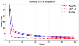
(a) GreatCourt Train Loss

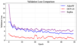
(b) GreatCourt Validation Loss

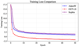
(c) KingsCollege Train Loss

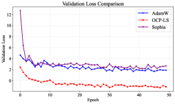
(d) KingsCollege Validation Loss

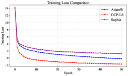
(e) OldHospital Train Loss

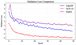
(f) OldHospital Validation Loss

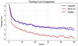
(g) ShopFacade Train Loss

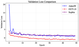
(h) ShopFacade Validation Loss

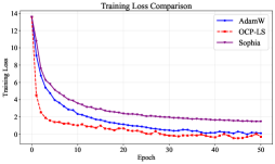
(i) StMarysChurch Train Loss

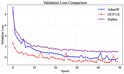
(j) StMarysChurch Validation Loss

Figure 1: Training and Validation Loss curves of the Cambridge Landmarks dataset

TABLE I: Comparison results of the six algorithms at 50 and 150 iteration steps

Dataset	Algorithm	Median Position Error	Mean Position Error	Median Rotation Error	Mean Rotation Error	$s^{p}$	$s^{q}$
GreatCourt	OCP-LS	11.847m	14.415m	9.794°	14.008°	1.452670	-2.709583
	AdamW	9.402m	12.299m	11.565°	20.804°	0.327468	-0.626888
	Sophia	10.345m	12.942m	12.356°	22.731°	0.061802	-0.061802
KingsCollege	OCP-LS	2.290m	2.784m	4.127°	5.240°	0.462569	-4.075670
	AdamW	2.506m	2.954m	5.743°	7.092°	0.168520	-0.465632
	Sophia	2.168m	2.875m	5.858°	7.037°	0.045892	-0.045892
OldHospital	OCP-LS	3.465m	4.160m	5.002°	6.222°	0.355842	-4.045096
	AdamW	3.809m	4.455m	7.927°	8.491°	0.369203	-1.729719
	Sophia	3.422m	4.148m	8.238°	8.989°	0.343930	-0.343930
ShopFacade	OCP-LS	2.276m	2.670m	7.839°	9.402°	0.423319	-2.955623
	AdamW	2.288m	2.788m	10.195°	10.684°	0.175533	-0.467277
	Sophia	2.244m	2.614m	10.006°	11.592°	0.047831	-0.047831
StMarysChurch	OCP-LS	3.226m	3.731m	7.683°	9.148°	0.902244	-3.125772
	AdamW	3.230m	3.727m	9.296°	12.121°	0.841389	-2.512417
	Sophia	2.918m	3.300m	12.768°	15.717°	0.388291	-0.388291

References

- [1] Kendall A, Grimes M, Cipolla R. Posenet: A convolutional network for real-time 6-dof camera relocalization[C]//Proceedings of the IEEE international conference on computer vision. 2015: 2938-2946.
- [2] Brahmbhatt S, Gu J, Kim K, et al. Geometry-aware learning of maps for camera localization[C]//Proceedings of the IEEE conference on computer vision and pattern recognition. 2018: 2616-2625.
- [3] Kendall A, Cipolla R. Geometric loss functions for camera pose regression with deep learning[C]//Proceedings of the IEEE conference on computer vision and pattern recognition. 2017: 5974-5983.
- [4] Zhang H, Wang H, Xu Y, et al. Optimization methods rooted in optimal control[J]. Science China Information Sciences, 2024, 67(12): 222208.
- [5] Wang H, Xu Y, Guo Z, et al. Optimization Algorithms with Superlinear Convergence Rate[J]. IEEE Transactions on Automatic Control, 2025.
- [6] Zhong J, Guo Z, Wang H, et al. An Efficient Algorithm for Learning-Based Visual Localization[J]. arXiv preprint arXiv:2511.04232, 2025.
- [7] Liu H, Li Z, Hall D L W, et al. Sophia: A Scalable Stochastic Second-order Optimizer for Language Model Pre-training[C]//The Twelfth International Conference on Learning Representations.