Higher-order response theory in stochastic thermodynamics and optimal control

Abstract

Linear response theory has found many applications in statistical physics. One of these is to compute minimal-work protocols that drive nonequilibrium systems between different thermodynamic states, which are useful for designing engineered nanoscale systems and understanding biomolecular machines. We compare and explore the relationships between linear-response-based approximations used to study optimal protocols in different driving regimes by showing that they arise as controlled truncations of a general causal response (Volterra) expansion. We then construct higher-order response terms and discuss the drawbacks and utility of their inclusion. We illustrate our results for an overdamped particle in a harmonic trap, ultimately showing that the inclusion of higher-order response in calculating optimal protocols provides marginal improvement in effectiveness despite incurring a significant computational expense, while introducing the possibility of predicting arbitrarily low and unphysical negative excess work.

I Introduction

A central goal of nonequilibrium thermodynamics is to characterize and calculate optimal, minimal-work protocols that transform a thermodynamic system between different states in finite-time [seifert2007, blaber2023optimal]. These protocols find applications in fields such as the engineering of nanoscopic devices [diana2013finite, zulkowski2014optimal, proesmans2020finite, proesmans2020optimal, whitelam2023train, schmiedl2007efficiency, martinez2017colloidal, martin2018extracting, abiuso2020optimal, brandner2020thermodynamic, frim2022optimal, frim2022geometric], and in understanding biophysical systems [geiger2010optimum, dellago2013computing, sivak2016thermodynamic, lucero2019optimal, blaber2022efficient, davis2024active, wareham2024multi]. However, exact, analytic optimal protocols exist only for the simplest systems, such as a Brownian particle in a harmonic potential [seifert2007]. Alternatively, a wide range of approximate results rely on assumptions based on linear response, which assumes that the thermodynamic system remains close to the driving protocol’s equilibrium state at all times [kubo1957, zwanzig2001nonequilibrium, limmer2022statmech]. These include the range of results from slow driving thermodynamic geometry [sivak2012, zulkowski2012geometry, rotskoff2015optimal, rotskoff2017geometric, zulkowski2015optimal, frim2022geometric, frim2022optimal], ansatz-based slow driving results [bonanca2014], and results applying in the weak driving regime [bonanca2018, naze2022optimal, naze2024analytical].

However, linear response represents only the first-order term of a higher order response expansion, or Volterra series. Our goal in this manuscript is both to clarify the basis of and relationships among linear response approximations as used in finite-time thermodynamics, and to study to higher order response in this context. While the Volterra series is well known in control theory [boyd1984analytical, BROCKETT1976167, wiener1942response, FRISTON20031273, lesiak1977], in physics it often appears implicitly such as in time-ordered response [kubo1957, zwanzig2001nonequilibrium] or Dyson expansions [Dyson1949]. Here, we use it as a clarifying framework to organize and compare existing linear-response approximations and to explore higher-order extensions.

We first demonstrate how existing linear response approaches such as thermodynamic geometry and ansatz-based weak driving are derived from the first term of the Volterra series. We also demonstrate the equivalence of linear-response thermodynamic geometry with the perturbative approach expressed in [wadia2022solution], and extend this perturbative solution to all orders for the overdamped moving harmonic oscillator, observing that including higher orders in the excess work cost function can lead to predictions of unphysical negative excess work, and that jumps found in true optimal protocols [seifert2007, zhong2024, aurell2011optimal, Aurell2012BoundaryLayers] can cause the series to diverge.

Following this, we construct next-order response terms in the context of finite-time thermodynamics. To evaluate the utility of using next-order correction beyond linear response to derive optimal finite-time protocols, we study quadratic response for an overdamped harmonic oscillator. We find that while including higher-order response terms can marginally improve the performance of derived optimal protocols, their inclusion comes at a substantial computational cost, and again allows for the possibility of predicting unphysical negative excess work.

These obstacles further motivate a different but related approach to optimal stochastic thermodynamics based on a recently discovered connection between optimal transport and thermodynamic geometry [zhong2024, ito2024geometric], which avoids relying on limited near-equilibrium expansions.

Preliminaries

The results of our manuscript are valid for passive (i.e., detailed-balance preserving) overdamped and underdamped Langevin dynamics, as well as passive discrete state Markov dynamics. Given a Hamiltonian $H_{\lambda}(x)$ parameterized by control-parameters $\lambda\in\mathcal{M}$, the expected work needed to implement a finite-time protocol $\Lambda=\lambda(t)|_{t\in[0,t_{f}]}$ connecting $\lambda(0)=\lambda_{i}$ to $\lambda(t_{f})=\lambda_{f}$ is given by

$$\langle W\rangle=\int_{0}^{t_{f}}\dot{\lambda}^{\mu}\bigg\langle\frac{\partial H_{\lambda}}{\partial\lambda^{\mu}}\bigg\rangle\,{\mathrm{d}t},$$ (1)

where we have suppressed the explicit time dependence of $\lambda$, $H$, and the average over the nonequilibrium distribution. Here we focus on the continuous case where $x\in\mathbb{R}^{d}$. For the discrete case $x\in\Omega$ where $\Omega$ represents a finite discrete state space, integrals over $x\in\mathbb{R}^{d}$ become sums over $x\in\Omega$ (e.g., as specified in [sawchuk2024dynamical]).

Here, $\mathcal{M}$ is a $k$-dimensional manifold. Throughout this paper we utilize the Einstein summation convention where repeated upper and lower indices denote implicit summation, and the dot denotes a total time derivative $\dot{\lambda}^{\mu}:={\mathrm{d}}\lambda^{\mu}/{\mathrm{d}t}$. Greek indices will indicate covariant expressions, while Latin indices will correspond to coordinate dependent expressions. The unadorned brackets $\langle\cdot\rangle$ denote a nonequilibrium expectation, (i.e., over trajectories $x(t)|_{t\in[0,t_{f}]}$ that start in equilibrium with $\lambda_{i}$ and evolve via some specified Langevin dynamics), while $\langle\cdot\rangle^{\mathrm{eq}}_{\lambda}$ denotes an expectation value over the equilibrium thermodynamic state corresponding to control parameters set to $\lambda$.

The probability distribution over the system’s microstates at equilibrium with respect to control parameters $\lambda$ is given by the canonical ensemble,

$$\rho^{\mathrm{eq}}_{\lambda}=\text{exp}\{-\beta[H_{\lambda}(x)-F(\lambda)]\}=\frac{e^{-\beta H_{\lambda}(x)}}{Z(\lambda)},$$ (2)

where $\beta$ is the inverse temperature, and $F$($\lambda$) = $-\beta^{-1}$ ln[$\int$exp$\{-\beta H_{\lambda}(x^{\prime})\}{\mathrm{d}x}^{\prime}$] is the free energy of the equilibrium state determined by $H_{\lambda}(x)$, which can written using the partition function $Z(\lambda)=\int\exp\{-\beta H_{\lambda}(x^{\prime})\}{\mathrm{d}x}^{\prime}$. Here we will only consider isothermal protocols. Because of this from here onward we set $\beta=1$ without loss of generality.

The time-evolution of the nonequilibrium probability density $\rho_{t}$ is governed by the following deterministic partial differential equation (PDE)

$$\frac{\partial\rho_{t}}{\partial t}=\mathcal{L}_{\lambda}[\rho_{t}],$$ (3)

where in the continuous case $\mathcal{L}_{\lambda}$ is the Fokker-Planck operator (for the discrete case, this would be the master equation and transition rate matrix).

We will assume that for any $\lambda$ defining the potential energy function the equilibrium distribution is the unique zero-mode of the Fokker-Planck operator

$$\mathcal{L}_{\lambda}[\rho^{\mathrm{eq}}_{\lambda}]=0,$$ (4)

and under the dynamics $\partial_{t}\rho_{t}=\mathcal{L}_{\lambda}[\rho_{t}]$ for a fixed $\lambda$, any arbitrary initial distribution $\rho_{0}$ will relax to the equilibrium distribution, $\lim_{t\rightarrow\infty}\rho_{t}=\rho^{\mathrm{eq}}_{\lambda}$.

Splitting the nonequilibrium probability density $\rho_{t}(x)$ into the equilibrium density $\rho^{\mathrm{eq}}_{\lambda}$ and nonequilibrium deviation $\delta\rho_{t}(x)$,

$$\rho_{t}(x)=\rho^{\mathrm{eq}}_{\lambda}(x)+\delta\rho_{t}(x),$$ (5)

where, since $\rho^{\mathrm{eq}}_{\lambda}(x)$ is the zero-mode of ${\mathcal{L}}_{\lambda}$ [Eq. (4)], we can rewrite the time evolution as

$$\frac{\partial\rho_{t}}{\partial t}=\mathcal{L}_{\lambda}[\delta\rho_{t}].$$ (6)

Using $\delta\rho_{t}$, we can distinguish average excess work from average total work. Inserting Eq. (5) into Eq. (1) we obtain

$$\langle W\rangle=\langle W_{\text{rev}}\rangle+\langle W_{\text{ex}}\rangle,$$ (7)

where the two terms are

$$\langle W_{\mathrm{rev}}\rangle=\int^{t_{f}}_{0}{\mathrm{d}t}\dot{\lambda}^{\mu}\int{\mathrm{d}}x\frac{\partial H_{\lambda}(x)}{\partial\lambda^{\mu}}\rho_{\lambda}^{\mathrm{eq}}(x),$$ (8)

$$\langle W_{\mathrm{ex}}\rangle=\int^{t_{f}}_{0}{\mathrm{d}t}\dot{\lambda}^{\mu}\int{\mathrm{d}}x\frac{\partial H_{\lambda}(x)}{\partial\lambda^{\mu}}\delta\rho_{t}(x).$$ (9)

Here, $\langle W_{\mathrm{rev}}\rangle$ is the reversible work, which is equal to the free energy difference $\Delta F=F(\lambda_{f})-F(\lambda_{i})$ between the equilibrium states defined by the initial and final control parameters $\lambda_{i}$ and $\lambda_{f}$, which is independent of the protocol between the initial and final points. $\langle W_{\mathrm{ex}}\rangle$ is the excess work, which is dependent on the shape and speed of the protocol.

Given that $\langle W_{\mathrm{rev}}\rangle=\Delta F$ is simply a function of the initial and final equilibrium states, our task becomes minimizing Eq. (9). The problem of minimizing average excess work can be broken into roughly four regimes where different approximations apply, corresponding to slow driving ($t_{f}$ is “large”), weak driving (the two equilibrium distributions specified by $\lambda_{i}$ and $\lambda_{f}$ are nearby in a suitable sense), simultaneously slow and weak driving, and driving which is neither slow nor weak, as illustrated in Fig. 1.

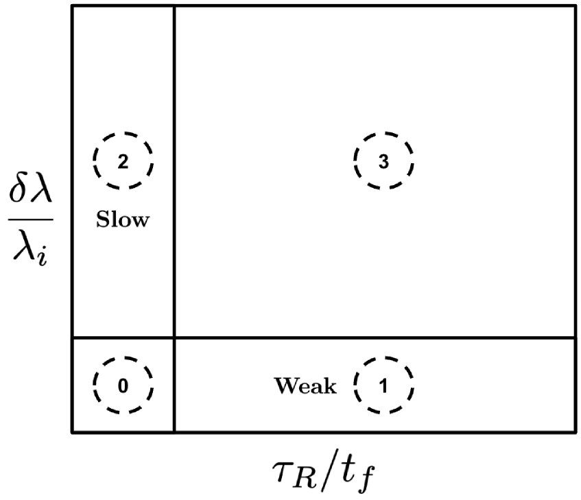
Figure 1: Approximation regimes in optimal stochastic thermodynamics. Following [dibyenduperscom, bonanca2018], we can parameterize the control protocol as $\lambda(t)=\delta\lambda(t)+\lambda_{i}$, and $\tau_{R}$ represents an appropriate relaxation time for the system. Region 1 corresponds to weak driving, region 2 corresponds to slow driving, and region 3 corresponds to protocols that drive the system further from equilibrium.

In the past, linear-response-based approaches have been developed to find the optimal protocol minimizing the excess work. For the slow-driving limit, [sivak2012] developed a Riemmanian-geometric based approach to calculate optimal protocols minimizing Eq. (1), showing that the excess work can be approximated by

$$\langle W_{\mathrm{ex}}\rangle\approx\int_{0}^{t_{f}}\dot{\lambda}^{\mu}\dot{\lambda}^{\nu}g_{\mu\nu}(\lambda(t))\,{\mathrm{d}t},$$ (10)

where $g_{\mu\nu}(\lambda)$ is the friction tensor that may be readily computed using equilibrium time-correlation functions as we detail below. This friction tensor can be interpreted as a Riemmanian metric on the space of control parameters $\lambda\in\mathcal{M}$, and under this interpretation, Eq. (10) is squared path divergence for the protocol $\Lambda$ in the geometry induced by $g_{\mu\nu}$. Thus, in this appropriate slow-driving limit, the optimal protocol is a geodesic connecting $\lambda_{i}$ and $\lambda_{f}$, yielding the excess cost as a squared thermodynamic length [crooks2007measuring] in this geometry.

Alternatively, [bonanca2018, naze2022optimal, naze2024analytical] have considered the weak driving limit, where $\delta\lambda(t)/\lambda_{i}$ is small, or $\lambda(t)\approx\lambda_{i}$ showing that the excess work may instead be expressed as

$$\langle W_{\mathrm{ex}}\rangle\approx\frac{1}{2}\int_{0}^{t_{f}}\int_{0}^{t_{f}}\dot{\lambda}^{a}(t)\,\Psi^{(1)}_{ab}(\lambda_{i};|t-t^{\prime}|)\,\dot{\lambda^{b}}(t^{\prime})\,{\mathrm{d}t}\,{\mathrm{d}t}^{\prime},$$ (11)

where $\Psi^{(1)}_{ab}(\lambda_{i};\tau)$ is the “relaxation function” at time-lag $\tau$ defined for $\lambda_{i}$, that may similarly be computed using an average over the initial equilibrium state, or constructed phenomenologically.

These approximations rely on low control parameter velocity in the slow driving case (regions 0 and 2 of Fig. 1), and low variations from the initial control parameters in the weak driving case (regions 0 and 1). As we will see, each of these results can be derived from the first order of a Volterra series.

One natural idea for attempting to extend approximations from regions 1 or 2 into region 3 (neither slow nor weak, further from equilibrium) is to include higher-order terms of the series approximation on which they depend. Both the weak and slow driving approximations rely on linear response: to extend them, we will consider including higher order response. First, we will introduce the Volterra series, discuss its application to optimal stochastic thermodynamics, and show how these approximations naturally arise from its first order.

II The Volterra Expansion of $\bm{\delta\rho_{t}}$

We can begin by suitably rewriting Eq. (9), then considering the response of the non-equilibrium correction $\delta\rho_{t}$ to changes in the underlying Hamiltonian. Defining the conjugate force with respect to control parameter $\lambda^{\mu}$ as

$$f_{\mu}(x):=-\frac{\partial H_{\lambda}(x)}{\partial\lambda^{\mu}}$$ (12)

we can write Eq. (9) as

$$\langle W_{\text{ex}}\rangle=-\int^{t_{f}}_{0}{\mathrm{d}t}\dot{\lambda}^{\mu}\int{\mathrm{d}x}f_{\mu}(x)\delta\rho_{t}(x).$$ (13)

Equivalently, because the normalization $\int\rho_{t}(x){\mathrm{d}x}=1$ and $\int\rho^{\mathrm{eq}}_{\lambda}(x){\mathrm{d}x}=1$ implies that $\int\delta\rho_{t}(x){\mathrm{d}x}=0$, the excess work can be rewritten as

$$\langle W_{\text{ex}}\rangle=-\int^{t_{f}}_{0}{\mathrm{d}t}\dot{\lambda}^{\mu}\int{\mathrm{d}}x\delta f_{\mu}(x)\delta\rho_{t}(x),$$ (14)

where

$$\delta f_{\mu}(x)=f_{\mu}(x)-\langle f_{\mu}\rangle^{\mathrm{eq}}_{\lambda}$$ (15)

is the excess conjugate force. Note that one can relate the excess conjugate force and the equilibrium probability density via the identity

$$\delta f_{\mu}(x)=\frac{\partial\ln\rho^{eq}_{\lambda}(x)}{\partial\lambda^{\mu}}.$$ (16)

Borrowing from control theory, $\delta\rho_{t}$ can be systematically approximated using a Volterra series [boyd1984analytical, BROCKETT1976167, wiener1942response, FRISTON20031273, lesiak1977]. The Volterra series considers the response of a dynamical system to a series of inputs. In finite-time thermodynamics, the system is driven between equilibria, where at each point it is pushed out of equilibrium to a variable extent. This suggests a natural identification of the vector of control parameter velocities $\dot{\lambda}$ as the input variables to the dynamical system, with the deviation from equilibrium being the output (as $\dot{\lambda}=0$ leads to $\delta\rho_{t}=0$). Given this identification, the Volterra series approximation for $\delta\rho_{t}$ is given by

$$\delta\rho_{t}(x)\approx\sum^{N}_{n=1}\int^{t}_{-\infty}.\int^{t}_{-\infty}\bigg\{\dot{\lambda}^{i_{1}}(t_{1})\cdot.\cdot\dot{\lambda}^{i_{n}}(t_{n})\cdot h^{(n)}_{i_{1}...i_{n}}(\lambda(t);t-t_{1},.,t-t_{n})\bigg\}\prod^{n}_{j=1}{\mathrm{d}t}_{j}.$$ (17)

Here $h^{(n)}_{i_{1}...i_{n}}(\lambda(t);t-t_{1},...,t-t_{n})$ is the $n^{\text{th}}$-order Volterra kernel defined at for the system fixed by control parameters $\lambda(t)$, which can be evaluated by considering $n$ impulses to the system at the timelags $t-t_{1},...,t-t_{n}$, as we shall explain below. (As a reminder, under Einstein summation notation each $i_{1}$, $i_{2}$, …, sums from $1$ to $k$, the dimensionality of the control space manifold $\mathcal{M}$.) Here, each Volterra kernel will be a function of position $h^{(n)}_{i_{1},....,i_{n}}(\lambda(t);...)(x)$ representing the response at each point $x$; however, for clarity the $x$-dependence will be suppressed. For lengthy expressions, the $x$-dependence of conjugate forces $\delta f(x)$ or probability densities $\rho(x)$ will be similarly suppressed.

II.1 First Order - Linear Response

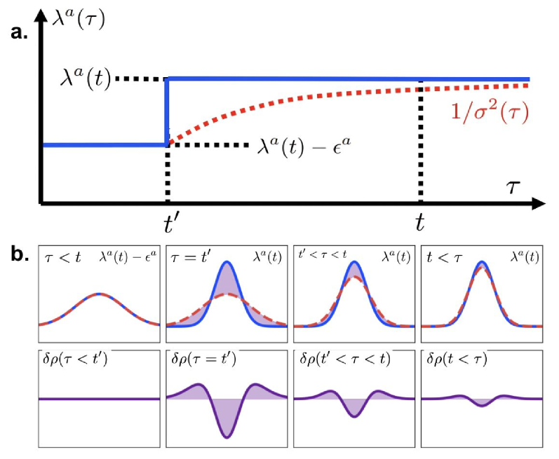
Figure 2: Derivation of the linear response function. a. The control parameter $\lambda^{a}$ moves from $\lambda^{a}(t)-\epsilon^{a}$ to $\lambda^{a}(t)$ at time $t^{\prime}$. If we assume $\lambda^{a}(\tau)=\alpha(\tau)$, where $\alpha(\tau)$ is the stiffness of a simple harmonic oscillator, the inverse variance of the nonequilibrium distribution, $1/\sigma^{2}(\tau<t^{\prime})$, is equal to $\alpha(\tau<t^{\prime})$ at equilibrium. Once the control parameter changes, $\delta\rho\neq 0$ and $1/\sigma^{2}(\tau)\neq\alpha(\tau)$. After this, over time $\delta\rho$ relaxes back to zero and $1/\sigma^{2}(\tau)$ relaxes to the new value, $\alpha(t)$. This picture is exact for the simple harmonic oscillator, but in general, this serves as a cartoon as the nonequilibrium density will not correspond to an equilibrium density for the same system for any control parameter value, requiring more than a single parameter to characterize their difference. b. The evolution of the nonequilibrium density $\rho(\tau)$ (dotted red line) is shown along with the equilibrium density $\rho^{\mathrm{eq}}(\tau)$ (solid blue line) corresponding to the current control parameter value (as specified in the upper right corner of the upper panels), with their difference indicated by the purple shaded area. In the bottom panels, assuming $\lambda^{a}(\tau)=\alpha(\tau)$, the stiffness of a simple harmonic oscillator, the equilibrium distribution defined by the potential abruptly changes from $\rho^{\mathrm{eq}}_{\lambda^{a}(t)-\epsilon^{a}}$ to $\rho^{\mathrm{eq}}_{\lambda^{a}(t)}$. Initially $\delta\rho=0$. After $\tau=t^{\prime}$, $\delta\rho$ decays back to zero as $\rho(\tau)\rightarrow\rho^{\mathrm{eq}}(t)$.

In this section we show how both thermodynamic geometry and weak-driving linear-response approximations [Eqs. (10) and (11)] can be derived from this Volterra series expansion truncated at $N=1$. The nonequilibrium correction given by first-order response is defined as

$$\delta\rho^{(1)}_{t}=\int^{t}_{-\infty}h^{(1)}_{a}(\lambda(t);t-t_{1})\dot{\lambda}^{a}(t_{1}){\mathrm{d}t}_{1}.$$ (18)

The first-order Volterra kernel (equivalently called first-order or linear response function) $h^{(1)}$ can be evaluated by considering the system’s first-order response to a single jump perturbation. This jump perturbation in the control parameter $\lambda^{a}$ can be expressed as

$$\dot{\lambda}^{a}(\tau)=\epsilon^{a}\delta(\tau-t^{\prime}).$$ (19)

This corresponds to a simple step in a control parameter $\lambda^{a}$ at time $t^{\prime}$, from $\lambda^{a}(t)-\epsilon^{a}$ to $\lambda^{a}(t)$ (where $\lambda(t)$ is the vector of control parameters at time $t>t^{\prime}$). We can find the first-order response function by evaluating the response of $\delta\rho_{t}$ to this change, to first order in $\epsilon^{a}$ (see Fig. 2).(a).

The nonequilibrium correction just after the jump, $\delta\rho_{t^{\prime}}(x)$, is given by $\delta\rho_{t^{\prime}}(x)=\rho^{\mathrm{eq}}_{\lambda(t)-\epsilon}(x)-\rho^{\mathrm{eq}}_{\lambda(t)}(x)$, where $\rho^{\mathrm{eq}}_{\lambda(t)-\epsilon}(x)$ is the equilibrium distribution before the perturbation, and $\epsilon$ is a vector with just one non-zero term, equal to $\epsilon^{a}$.

Linearizing with $\partial_{\lambda^{a}}(\rho^{\mathrm{eq}}_{\lambda})=\rho^{\mathrm{eq}}_{\lambda}\,(\partial_{\lambda^{a}}\ln\rho^{\mathrm{eq}}_{\lambda})=\rho^{\mathrm{eq}}_{\lambda}\delta f_{a}$ (using Eq. (16), with $\partial_{\lambda^{a}}=\partial/\partial\lambda^{a}$), we have

$$\rho^{\mathrm{eq}}_{\lambda(t)-\epsilon} =\rho^{\mathrm{eq}}_{\lambda(t)}-\epsilon^{a}\partial_{\lambda^{a}}(\rho^{\mathrm{eq}}_{\lambda(t)})+\mathcal{O}((\epsilon^{a})^{2})$$ (20)

$$=\rho^{\mathrm{eq}}_{\lambda(t)}[1-\epsilon^{a}\delta f_{a}]+\mathcal{O}((\epsilon^{a})^{2}).$$ (21)

To approximate $\delta\rho_{t}$, we apply the time evolution operator exp$({\mathcal{L}}_{\lambda}(t-t^{\prime}))$ to $\delta\rho_{t^{\prime}}$ to obtain $\delta\rho_{t}$ up to linear order:

$$\delta\rho_{t} =\text{ exp}({\mathcal{L}}_{\lambda}(t-t^{\prime}))[\rho^{\mathrm{eq}}_{\lambda(t)}-\rho^{\mathrm{eq}}_{\lambda(t)-\epsilon}]$$ (22)

$$\approx-\epsilon^{a}\text{exp}({\mathcal{L}}_{\lambda}(t-t^{\prime}))\rho^{\mathrm{eq}}_{\lambda(t)}\delta f_{a}.$$

Inserting Eq. (19) into Eq. (18)

$$\delta\rho_{t}^{(1)}=-\epsilon^{a}h^{(1)}_{a}(\lambda(t);t-t^{\prime}),$$ (23)

we find the first-order response function for $\delta\rho_{t}$ to be

$$h^{(1)}_{a}(\lambda(t);\tau)=\exp({\mathcal{L}}_{\lambda}\tau)[\rho^{\text{eq}}_{\lambda(t)}\delta f_{a}].$$ (24)

With this, we can write out the excess work assuming linear response, $\langle W_{\text{ex}}^{(1)}\rangle$, by replacing $\delta\rho_{t}$ in Eq. (14) with $\delta\rho_{t}^{(1)}$ with the above approximations

$$\langle W_{\text{ex}}^{(1)}\rangle =\int^{t_{f}}_{0}{\mathrm{d}t}\dot{\lambda}^{a}(t)\underbrace{\int^{t}_{-\infty}{\mathrm{d}t}_{1}\dot{\lambda}^{b}(t_{1})\bigg\{\int{\mathrm{d}}x\delta f_{a}(x)\text{exp}({\mathcal{L}}_{\lambda}(t-t_{1}))[\delta f_{b}(x)\rho^{\mathrm{eq}}_{\lambda}(x)]\bigg\}}_{\int\delta f_{a}(x)\delta\rho_{t}^{(1)}(x){\mathrm{d}x}}$$ (25)

$$=\int^{t_{f}}_{0}{\mathrm{d}t}\dot{\lambda}^{a}(t)\int^{t}_{-\infty}{\mathrm{d}t}_{1}\dot{\lambda}^{b}(t_{1})\Psi_{ab}^{(1)}(\lambda(t);t-t_{1}).$$

This formula can be matched to previous results where linear response is introduced by observing that the relaxation function (as defined by Eq. (25)) is the excess conjugate force correlation function

$$\Psi_{ab}^{(1)}(\lambda(t);\tau)= \int{\mathrm{d}}x\delta f_{a}(x)e^{{\mathcal{L}}_{\lambda}\tau}[\delta f_{b}(x)\rho^{\mathrm{eq}}_{\lambda}(x)]$$ (26)

$$=\langle\delta f_{a}(0)\delta f_{b}(\tau)\rangle^{\mathrm{eq}}_{\lambda(t)}.$$

From this expression, we can derive thermodynamic geometry and the weak-driving approximations.

II.1.1 Low Acceleration Limit (Thermodynamic Geometry)

With an additional assumption, the results from thermodynamic geometry can be derived from the first-order term of the Volterra series of $\delta\rho_{t}$. By Taylor-expanding the control parameter velocity around its value at $t$ and assuming the acceleration of control parameters is small, we arrive at the thermodynamic geometry results used in [sivak2012, zulkowski2012geometry, rotskoff2015optimal, rotskoff2017geometric, zulkowski2015optimal, frim2022geometric, frim2022optimal]. This additional step means thermodynamic geometry assumes slow driving by taking the first term of the Volterra series, and low acceleration driving by using the expansion

$$\dot{\lambda}(t_{1})=\dot{\lambda}(t)+\mathcal{O}(\ddot{\lambda}(t)),$$ (27)

which gives us

$$\langle W_{\text{ex}}^{(1)}\rangle\approx\int^{t_{f}}_{0}{\mathrm{d}t}\dot{\lambda}^{\mu}(t)\dot{\lambda}^{\nu}(t)\int^{t}_{-\infty}{\mathrm{d}t}_{1}\Psi_{ab}^{(1)}(\lambda(t);t-t_{1}).$$ (28)

Changing variables to $\tau_{1}=t-t_{1}$, we can rewrite the integral on the right of the above expression as the friction tensor,

$$\zeta^{(1)}_{\mu\nu}(\lambda(t)) =\int^{\infty}_{0}d\tau\Psi_{ab}^{(1)}(\lambda(t);\tau)$$ (29)

$$=\int^{\infty}_{0}d\tau\langle\delta f_{\mu}(0)\delta f_{\nu}(\tau)\rangle^{\mathrm{eq}}_{\lambda(t)}$$

$$\langle W_{\text{ex}}^{(1)}\rangle\approx\int^{\tau}_{0}{\mathrm{d}t}\dot{\lambda}^{\mu}(t)\dot{\lambda}^{\nu}(t)\zeta^{(1)}_{\mu\nu}(\lambda(t)),$$ (30)

which can be used to define a metric on the space of thermodynamic states. Geodesics of this metric provide optimal protocols assuming both low control parameter acceleration and low control parameter velocity. This offers a computationally inexpensive way to calculate optimal protocols, but its near-optimality in performance is only guaranteed if these assumptions are satisfied.

In the overdamped limit, a slow-driving metric on the space of thermodynamic states can also be derived through a perturbative expansion using the Green’s function [Wadia_2022]: $\delta\rho_{t}=\delta\rho_{t}^{(1),P}+\delta\rho_{t}^{(2),P}+...$, where

$$\delta\rho_{t}^{(1),P}=\mathcal{L}_{\lambda(t)}^{-1}[\partial_{t}\rho^{\mathrm{eq}}_{\lambda(t)}]$$ (31)

and $\delta\rho_{t}^{(\ell+1),P}=\mathcal{L}_{\lambda(t)}^{-1}[\partial_{t}\delta\rho_{t}^{(\ell),P}]$. Here, $\mathcal{L}_{\lambda(t)}^{-1}$ is the Green’s function of the Fokker-Planck operator, which is also known as the Drazin inverse [mandal2016analysis, sawchuk2024dynamical]. In Appendix A, we demonstrate that the metric from this approach is equivalent to Eq. (29) using a spectral decomposition as performed in [sawchuk2024dynamical].

In Appendix B, we derive all orders of the perturbative expansion for an overdamped moving harmonic trap, observing that the inclusion of higher orders can lead to unphysical negative excess work if evaluated outside its slow-driving range of applicability, while true optimal protocols that include finite jumps [seifert2007, zhong2024, aurell2011optimal, Aurell2012BoundaryLayers] can lead the first term in the series to diverge.

II.1.2 Weak Driving Limit

The weak driving result from [bonanca2018] can be derived from a simple change to the first term in the Volterra series Eq. (25). $\Psi_{ab}^{(1)}(\lambda(t);t-t_{1})$ is approximated by an ansatz defined by the initial state of the system. In the overdamped limit this is given by

$$\Psi_{ab}^{(1)}(\lambda(t);\tau_{1})\approx\Psi_{ab}^{(1)}(\lambda(0);0)\cdot\exp(-s|\tau_{1}|),$$ (32)

where $s$ is a phenomenological parameter [bonanca2018]. This is computationally advantageous since the left hand side of Eq. (32) is dependent on both $t$ and $|t-t_{1}|$, whereas the right hand side depends only on $|t-t_{1}|$. Expanding the protocol with a set of basis functions, $\langle W_{\text{ex}}^{(1)}\rangle$ can be rewritten in terms of the protocol’s basis coefficients, which is possible because the ansatz is independent of $\lambda(t)$. In this case $\langle W_{\text{ex}}^{(1)}\rangle$ can be efficiently optimized since only the basis coefficients need to be varied.

The ansatz setting the dependence on $\tau_{1}$ is further discussed in [bonanca2014]. However, in this case we can consider the spectral properties of the Fokker-Planck operator to assess the validity of this ansatz. In the weak driving limit we can simply say $\lambda(t)\approx\lambda(0)$, so that

$$\Psi_{ab}^{(1)}(\lambda(t);\tau_{1})\approx\Psi_{ab}^{(1)}(\lambda(0);\tau_{1}).$$ (33)

Recalling Eq. (25), we can notice that the dependence on $\tau_{1}$ will be inherited from the exponential Fokker-Planck operator. If $\partial\rho^{\mathrm{eq}}_{\lambda}(x)/\partial\lambda^{b}=\delta f_{b}(x)\rho^{\mathrm{eq}}_{\lambda}(x)$ is an eigenvector of the Fokker-Planck operator, the relaxation function will be a simple exponential with $s$ equaling the corresponding eigenvalue. As we will see in Section III, this is true for an overdamped particle in a simple harmonic oscillator. However, if $\delta f_{b}(x)\rho^{\mathrm{eq}}_{\lambda}(x)$ is not an eigenvector of ${\mathcal{L}}_{\lambda}$, this ansatz will be less appropriate.

It is interesting to note that [naze2024analytical] found that for cost functions of the form Eq. (11), no matter the form of $\Psi_{ab}^{(1)}$, as long as it is a positive kernel that us unchanging over the protocol as given by the weak-driving assumption, exact solutions are always symmetric in time. This point is reflected in our numerical results in Section III.

II.2 Second Order - Quadratic Response

Next we turn to higher-order terms in the Volterra expansion for $\delta\rho_{t}$. These can be computed by considering the response to a sequence of steps rather than one as in the linear response case. Here, we focus on evaluating the next order response, which can be computed by considering the relaxation from two step changes to the system, and evaluating the resulting expression to second order in the step size. We can express the quadratic response correction as

$$\delta\rho^{(2)}_{t}(x) =\int_{-\infty}^{t}h_{a}^{(1)}(\lambda(t);t-t_{1})\dot{\lambda}^{a}(t_{1})\,{\mathrm{d}t}_{1}$$ (34)

$$+\int_{-\infty}^{t}\int_{-\infty}^{t} h_{ab}^{(2)}(\lambda(t);t-t_{1},t-t_{2})\dot{\lambda}^{a}(t_{1})\dot{\lambda}^{b}(t_{2})\,{\mathrm{d}t}_{1}\,{\mathrm{d}t}_{2}.$$

Assuming the systems starts in equilibrium, we can consider perturbing two control parameters, which move from $\lambda^{a}(t)-\epsilon_{1}^{a}$ to $\lambda^{a}(t)$ at $t^{\prime}$, and from to $\lambda^{b}(t)-\epsilon_{2}^{b}$ to $\lambda^{b}(t)$ at $t^{\prime\prime}$

$$\dot{\lambda}^{a}(\tau)=\epsilon_{1}^{a}\delta(\tau-t^{\prime}),\,\,\,\dot{\lambda}^{b}(\tau)=\epsilon_{2}^{b}\delta(\tau-t^{\prime\prime}).$$ (35)

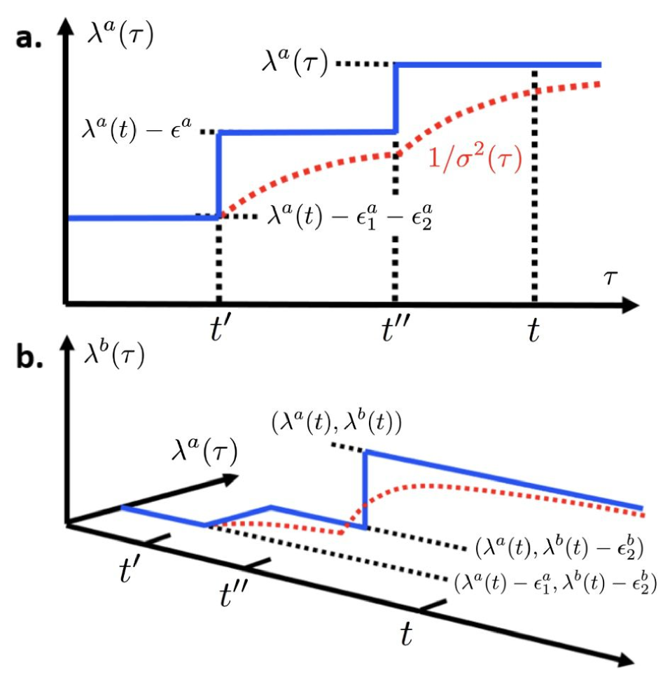
Figure 3: Derivation of the quadratic response function. a. Response of the system (dotted red line) to two perturbations of a single control parameter $\lambda^{a}$ (solid blue line). For example, if the control parameter were the stiffness of a harmonic oscillator, the inverse variance of the nonequilibrium distribution would react to changes in this parameter. Again, this picture serves as a cartoon for systems with densities not fully characterized by a single parameter. b. We also consider perturbations to each of two different control parameters, $\lambda^{a}$ and $\lambda^{b}$.

We will use a subscript shorthand for the control parameter at the time $t$, $\lambda(t)=\lambda_{0}$. $\rho^{\mathrm{eq}}_{\lambda(t)}=\rho^{\mathrm{eq}}_{0}$, ${\mathcal{L}}_{\lambda}=\mathcal{L}_{0}$, and $\int(\cdot)\rho^{\mathrm{eq}}_{\lambda(t)}{\mathrm{d}x}=\langle\cdot\rangle_{0}$. For the control setting between $t^{\prime}$ and $t^{\prime\prime}$ when just the control parameter $\lambda^{b}$ is perturbed, we will use $\rho^{\mathrm{eq}}_{\lambda^{b}(t)-\epsilon_{2}^{b}}=\rho^{\mathrm{eq}}_{b}$, $\mathcal{L}_{\lambda^{b}(t)-\epsilon_{2}^{b}}=\mathcal{L}_{b}$, and $\int(\cdot)\rho^{\mathrm{eq}}_{b}{\mathrm{d}x}=\langle\cdot\rangle_{b}$, whereas before $t^{\prime\prime}$ where both parameters $\lambda^{a}$ and $\lambda^{b}$ are perturbed, we’ll refer to the corresponding equilibrium distribution as $\rho^{\mathrm{eq}}_{a,b}$. Using these definitions we can write the deviation from equilibrium at the time $t>t^{\prime\prime}>t^{\prime}$ as

$$\delta\rho(t)= e^{\mathcal{L}_{0}(t-t^{\prime\prime})}\Big[\rho^{\mathrm{eq}}_{b}+e^{\mathcal{L}_{b}(t^{\prime\prime}-t^{\prime})}\big(\rho^{\mathrm{eq}}_{a,b}-\rho^{\mathrm{eq}}_{a}\big)\Big]-\rho^{\mathrm{eq}}_{0}.$$ (36)

This expression can be to quadratic order in the perturbations to obtain the second-order response function. First, we can compute the deviation from equilibrium directly after the first step at $t^{\prime}$, $\delta\rho_{t^{\prime}}=\rho^{\mathrm{eq}}_{a,b}-\rho^{\mathrm{eq}}_{b}$. Expanding $\rho^{\mathrm{eq}}_{a,b}$ to second order in terms of $\epsilon_{1}^{a}$ and applying

$$\partial_{\lambda^{a}}^{2}\rho^{\mathrm{eq}}=\rho^{\mathrm{eq}}((\delta f_{a})^{2}+\partial_{\lambda^{a}}(\delta f_{a})),$$ (37)

we obtain

$$\delta\rho_{t^{\prime}} =\bigg[\rho^{\mathrm{eq}}_{b}-\epsilon_{1}^{a}\partial_{\lambda^{a}}\rho^{\mathrm{eq}}_{b}+\frac{(\epsilon_{1}^{a})^{2}}{2}\partial_{\lambda^{a}}^{2}\rho^{\mathrm{eq}}_{b}+\mathcal{O}((\epsilon_{1}^{a})^{3})\bigg]-\rho^{\mathrm{eq}}_{b}$$ (38)

$$=\rho^{\mathrm{eq}}_{b} \bigg[-\epsilon_{1}^{a}\delta f_{a}^{(b)}+\frac{(\epsilon_{1}^{a})^{2}}{2}[(\delta f_{a}^{(b)})^{2}+\partial_{\lambda^{a}}(\delta f_{a}^{(b)})]+\mathcal{O}((\epsilon_{1}^{a})^{3})\bigg],$$

with $\delta f_{a}^{(b)}$ being the excess conjugate force evaluated with respect to the control setting between $t^{\prime\prime}$ and $t^{\prime}$. Keeping our expansion to second order in $\epsilon_{1}^{a}$ and $\epsilon_{2}^{b}$, we can expand $\delta f_{a}^{(b)}$ to first order in $\epsilon_{2}^{b}$

$$\delta f_{a}^{(b)}=\delta f_{a}-\epsilon_{2}^{b}\partial_{\lambda^{b}}\delta f_{a}+\mathcal{O}((\epsilon_{2}^{b})^{2}),$$ (39)

and expanding $\rho^{\mathrm{eq}}_{b}$ around $\lambda(t)$ as

$$\rho^{\mathrm{eq}}_{b}=\rho^{\mathrm{eq}}_{0}\Big(1-\epsilon_{2}^{b}\delta f_{b}+\frac{(\epsilon_{2}^{b})^{2}}{2}[\delta f_{b}^{2}+\partial_{\lambda^{b}}(\delta f_{b})]\Big)+\mathcal{O}((\epsilon_{2}^{b})^{3}),$$ (40)

we can insert Eq. (39) into Eq. (38) and take the first order of Eq. (40) to evaluate Eq. 38. We find

$$\delta\rho_{t^{\prime}} =\rho^{\mathrm{eq}}_{0}(-\epsilon_{1}^{a}\delta f_{a}+\epsilon_{1}^{a}\epsilon_{2}^{b}[\delta f_{a}\delta f_{b}+\partial_{\lambda_{b}}(\delta f_{a})]$$ (41)

$$+\frac{(\epsilon_{1}^{a})^{2}}{2}[(\delta f_{a})^{2}+\partial_{\lambda^{a}}(\delta f_{a})])+\mathcal{O}(\epsilon^{3}),$$

where $\mathcal{O}(\epsilon^{3})$ represents the sum of all terms of 3rd order or higher in $\epsilon_{1}^{a}$ and/or $\epsilon_{2}^{b}$. To finish writing Eq. (36) in terms of $\lambda_{0}$ we expand $e^{\mathcal{L}_{b}(t^{\prime\prime}-t^{\prime})}$ to first order in $\epsilon_{2}^{b}$

$$e^{\mathcal{L}_{b}(t^{\prime\prime}-t^{\prime})}=e^{\mathcal{L}_{0}(t^{\prime\prime}-t^{\prime})}+\epsilon_{2}^{b}\partial_{\lambda^{b}}\Big[e^{\mathcal{L}_{0}(t^{\prime\prime}-t^{\prime})}\Big]+\mathcal{O}((\epsilon_{2}^{b})^{2}).$$ (42)

Inserting Eqs. (40),  (41), and  (42) into Eq. (36) we find that

$$\begin{gathered}\delta\rho(t)=\bigg\{-\epsilon_{1}^{a}[e^{\mathcal{L}_{0}(t-t^{\prime})}(\delta f_{a}\rho^{\mathrm{eq}}_{0})]-\epsilon_{2}^{b}[e^{\mathcal{L}_{0}(t-t^{\prime\prime})}(\delta f_{b}\rho^{\mathrm{eq}}_{0})]\bigg\}+\bigg\{\frac{(\epsilon_{1}^{a})^{2}}{2}\big[e^{\mathcal{L}_{0}(t-t^{\prime})}(\delta f_{a}^{2}+\partial_{\lambda^{a}}(\delta f_{a}))\rho^{\mathrm{eq}}_{0}\big]+\frac{(\epsilon_{2}^{b})^{2}}{2}\big[e^{\mathcal{L}_{0}(t-t^{\prime\prime})}(\delta f_{b}^{2}\\ +\partial_{\lambda^{b}}(\delta f_{b}))\rho^{\mathrm{eq}}_{0}\big]+\epsilon_{1}^{a}\epsilon_{2}^{b}\big[e^{\mathcal{L}_{0}(t-t^{\prime})}(\delta f_{a}\delta f_{b}+\partial_{\lambda^{b}}(\delta f_{a}))\rho^{\mathrm{eq}}_{0}\big]+\epsilon_{1}^{a}\epsilon_{2}^{b}\Big[e^{\mathcal{L}_{0}(t-t^{\prime\prime})}\big[\partial_{\lambda^{b}}e^{\mathcal{L}_{0}(t^{\prime\prime}-t^{\prime})}\big]\delta f_{a}\rho^{\mathrm{eq}}_{0}\Big]\bigg\}+\mathcal{O}(\epsilon^{3}).\end{gathered}$$ (43)

As was done for the linear response case, we can insert the jump perturbation velocity expressed by (35) to Eq. (34), and match this to Eq. (43). The first two terms again recover the linear response function Eq. (24), while the following four terms give us the quadratic response function. From this expression we see that the quadratic response terms are higher order in terms of the deviation from equilibrium. For weak protocols, this confirms that the quadratic response terms will be small. The resulting quadratic response function is

$$h_{ab}^{(2)}(\lambda_{0};t-t^{\prime},t-t^{\prime\prime})=\frac{1}{2}\Big(e^{\mathcal{L}_{0}(t-t^{\prime})}[\delta f_{a}\delta f_{b}$$ (44)

$$+\partial_{\lambda^{b}}(\delta f_{a})]\rho^{\mathrm{eq}}_{0}+e^{\mathcal{L}_{0}(t-t^{\prime\prime})}\partial_{\lambda^{b}}[e^{\mathcal{L}_{0}(t^{\prime\prime}-t^{\prime})}]\delta f_{a}\rho^{\mathrm{eq}}_{0}\Big).$$

By inserting Eqs. (34) and (44) into Eq. (14), the next-order relaxation function $\Psi^{(2)}_{abc}=\int dx\,\delta f_{a}h^{(2)}_{bc}$ for $\tau_{1}>\tau_{2}$, we obtain

$$\begin{gathered}\Psi^{(2)}_{abc}(\lambda(t);\tau_{1},\tau_{2})=\frac{1}{2}\int{\mathrm{d}}x\,\delta f_{a}(x)\Big[e^{{\mathcal{L}}_{\lambda}\tau_{1}}[\delta f_{b}(x)\delta f_{c}(x)+\partial_{\lambda^{c}}[\delta f_{b}](x)]\rho^{\mathrm{eq}}_{\lambda(t)}+e^{{\mathcal{L}}_{\lambda}\tau_{2}}\partial_{\lambda^{c}}[e^{\mathcal{L}_{0}(\tau_{1}-\tau_{2})}]\rho^{\mathrm{eq}}_{\lambda(t)}\delta f_{b}(x)\Big]\\ \\ =\big\langle\delta f_{a}(\tau_{1})\delta f_{b}(0)\delta f_{c}(0)\big\rangle^{\mathrm{eq}}_{\lambda(t)}+\big\langle\delta f_{a}(\tau_{1})\partial_{\lambda^{c}}[\delta f_{b}](0)\big\rangle^{\mathrm{eq}}_{\lambda(t)}+\int_{0}^{\tau_{1}-\tau_{2}}\big\langle\delta f_{a}(\tau_{2})\delta S_{c}(\tau^{\prime})\delta f_{b}(0)\big\rangle^{\mathrm{eq}}_{\lambda(t)}\text{ }d\tau^{\prime},\end{gathered}$$ (45)

where the integral arises from the derivative of the exponential Fokker-Planck operator. $\delta S_{c}(\tau^{\prime})$, for a given trajectory, is defined as the change in log likelihood of the stochastic trajectory probability (in a Onsager-Machlup path action sense [adib2008stochastic]), given a perturbation in the gradient of the conjugate force $\nabla f_{b}(x(\tau^{\prime}))$ at time $\tau^{\prime}$.

Including the quadratic term in the Volterra Series in our approximation for the work $\langle W_{\mathrm{ex}}\rangle\approx\langle W_{\text{ex}}^{(1)}\rangle+\langle W_{\text{ex}}^{(2)}\rangle$, where Eq. (25) additionally with

$$\langle W_{\text{ex}}^{(2)}\rangle=\int^{t_{f}}_{0}{\mathrm{d}t}\dot{\lambda}^{a}(t)\int^{t}_{-\infty}{\mathrm{d}t}_{1}\dot{\lambda}^{b}(t_{1})\int_{-\infty}^{t_{1}}{\mathrm{d}t}_{2}\dot{\lambda}^{c}(t_{2})\Psi_{abc}^{(2)}(\lambda(t);t-t_{1},t-t_{2}),$$ (46)

allows us to compute the next order correction to optimal protocols.

Explicitly computing the quadratic term helps clarify exactly why linear response approaches apply only in regions 0, 1, and 2 of Fig. 1. Eq. (34) shows that higher orders of the Volterra Series are of higher order in the control parameter velocity $\dot{\lambda}$. Slower manipulation of the control parameters will allow the linear term to dominate. Eq. (43) shows that higher orders of the Volterra Series contribute only for higher orders of perturbation strength $\epsilon$, meaning weaker manipulation of control parameters allow the linear term to dominate.

III Linear and Quadratic Response of the Overdamped Harmonic Oscillator

These approximations can be evaluated by focusing on the overdamped harmonic oscillator, which has analytic results for comparison [seifert2007]. Considering overdamped Langevin dynamics, with the system’s microstate $x(t)\in\mathbb{R}$ and Gaussian white noise of unit amplitude $\eta(t)$, the system’s trajectory is given by

$$\gamma\dot{x}(t)=-\frac{\partial V_{\lambda}(x)}{\partial x}+\sqrt{2\gamma\beta^{-1}}\eta(t),$$ (47)

where $\gamma$ is the damping coefficient and $V_{\lambda}$ is the potential energy defined by control parameters $\lambda$. Since we will only consider protocols with constant temperature and damping coefficient, without loss of generality we set $\gamma=1$ and $\beta$ = 1. In the overdamped case the linear Fokker-Planck operator ${\mathcal{L}}_{\lambda}$ is given by

$${\mathcal{L}}_{\lambda}[\rho]=\frac{\partial}{\partial x}\left[\frac{\partial V_{\lambda}}{\partial x}+\frac{\partial}{\partial x}\right]\rho.$$ (48)

For the overdamped harmonic case, we can evaluate Eqs. (26) and (45) by writing these expressions in terms of left $\rho_{l,n}(x)$ and right $\rho_{r,n}(x)$ eigenvectors of the Fokker-Planck operator, given by

$$\mathcal{L}_{\lambda}\rho_{r,n}(x)=r_{n}\rho_{r,n}(x),$$ (49)

$${\mathcal{L}}_{\lambda}^{\dagger}\rho_{l,n}(x)=r_{n}\rho_{l,n}(x),$$ (50)

which can be shown to satisfy

$$\rho_{r,n}(x)=\rho^{\mathrm{eq}}_{\lambda(t)}\rho_{l,n}(x),$$ (51)

and form a complete, orthonormal basis [Wadia_2022]

$$\delta(x-y)=\sum_{n}\rho_{r,n}(x)\rho_{l,n}(y),$$ (52)

$$\int{\mathrm{d}x}\,\rho_{r,n}(x)\rho_{l,m}(x)=\delta_{nm}.$$ (53)

For a one-dimensional harmonic oscillator with variable stiffness and center location

$$V_{\lambda(t)}=\frac{\alpha(t)(x-\mu(t))^{2}}{2},$$ (54)

where $\lambda(t)=\big(\alpha(t),\mu(t)\big)$, the left eigenfunctions are

$$\rho_{l,n}=\frac{1}{\sqrt{n!}}\,\text{He}_{n}(\sqrt{\alpha(t)}(x-\mu(t))),$$ (55)

with the eigenvalues

$$r_{n}=-\alpha(t)\cdot n\quad\mathrm{for}\quad n=0,1,...$$ (56)

where He_n represents the $n^{\mathrm{th}}$ probabilist’s Hermite polynomial [wadia2022solution]. We can evaluate the response functions by applying the action of the Fokker-Planck time evolution operator on the right eigenfunctions

$$e^{{\mathcal{L}}_{\lambda}\tau}\rho_{r,n}= \sum^{\infty}_{n=0}e^{-r_{m}\tau}\rho_{r,m}(x)\int dy\,\rho_{l,m}(y)\,\rho_{r,n}(y)$$ (57)

$$= \,\,e^{-\alpha(t)n\tau}\rho_{r,n},$$

where we have used Eq. (53).

Since the eigenfunctions form a complete basis, we can evaluate the response functions by using an eigenfunction expansion. For the linear response function, Eq. (24), the time evolution operator acts on the conjugate force. In the moving and stiffening harmonic case, the conjugate forces Eq. (15) are given by

$$\delta f_{\alpha}(x)=\frac{\rho_{l,2}(x)}{\alpha\sqrt{2}}\quad\mathrm{and}\quad\delta f_{\mu}(x)=\sqrt{\alpha}\,\rho_{l,1}(x).$$ (58)

Inserting Eq. (58) into Eq. (26) and applying Eqs. (57) and (53), we obtain the linear relaxation functions:

$$\bm{\Psi}^{(1)}(\lambda(t);\tau)=\begin{pmatrix}\frac{1}{2\alpha^{2}}e^{-2\alpha\,\tau}&0\\ 0&\alpha\,e^{-\alpha\,\tau}\end{pmatrix}.$$ (59)

This agrees with the low acceleration results for the friction tensor obtained elsewhere [Wadia_2022, sivak2012, zulkowski2012] by applying Eq. (29) to obtain

$$\zeta^{(1)}(\lambda(t))=\begin{pmatrix}\frac{1}{4\alpha^{3}}&0\\ 0&1\end{pmatrix}.$$ (60)

For the quadratic response functions, we can apply the product rule to Eq. (44) to move the derivative off of the time-evolution operator

$$\Psi^{(2)}_{abc}(\lambda(t);\tau_{1},\tau_{2})=\int{\mathrm{d}x}\,\delta f_{a}(x)e^{{\mathcal{L}}_{\lambda}\tau_{1}}[\delta f_{b}(x)\delta f_{c}(x)+\partial_{\lambda^{b}}[\delta f_{c}](x)]\rho^{\mathrm{eq}}_{\lambda}$$ (61)

$$+\int{\mathrm{d}x}\,\delta f_{a}(x)e^{{\mathcal{L}}_{\lambda}\tau_{2}}\frac{\partial}{\partial\lambda_{b}}\Big[e^{{\mathcal{L}}_{\lambda}(\tau_{1}-\tau_{2})}\rho^{\mathrm{eq}}_{\lambda}\delta f_{c}(x)\Big]-\int{\mathrm{d}x}\,\delta f_{a}(x)e^{{\mathcal{L}}_{\lambda}\tau_{1}}\frac{\partial}{\partial\lambda_{b}}\Big[\rho^{\mathrm{eq}}_{\lambda}\delta f_{c}(x)\Big].$$

Whenever the time evolution operator is applied, we can first expand the function on which it operates in terms of right eigenfunctions of the Fokker-Planck operator.

By inserting Eq. (58) into Eq. (61) and applying Eqs. (57) and (53), we can evaluate the quadratic relaxation functions. For $\tau_{1}>\tau_{2}$, these are

$$\bm{\Psi}_{\alpha}^{(2)}(\lambda(t);\tau_{1},\tau_{2})=\begin{pmatrix}\frac{(1-\alpha(\tau_{1}-\tau_{2}))}{2\alpha^{3}}&0\\ 0&\frac{1}{2}\end{pmatrix}\cdot e^{-2\alpha\tau_{1}},$$ (62)

$$\bm{\Psi}_{\mu}^{(2)}(\lambda(t);\tau_{1},\tau_{2})=\begin{pmatrix}0&0\\ 1-\frac{\alpha(\tau_{1}-\tau_{2}))}{2}&0\end{pmatrix}\cdot e^{-\alpha\tau_{1}}.$$ (63)

(Here we have used the notation $\Psi_{i}=[[\Psi_{i\alpha\alpha},\Psi_{i\alpha\mu}]^{T},[\Psi_{i\mu\alpha},\Psi_{i\mu\mu}]^{T}]$.).

The low acceleration approximation can be to this expression and compared with previous results from Blaber and Sivak [blaber2020skewed], who derived a $\dot{\lambda}^{3}$ term by applying linear response to the squared excess work $\frac{\mathrm{d}}{{\mathrm{d}t}}\langle W_{\mathrm{ex}}^{2}\rangle$ and using Crooks’ fluctuation theorem [crooks1999entropy, crooks2000path]. We can obtain the next-order tensor by expanding both $\dot{\lambda}(t_{1})$ and $\dot{\lambda}(t_{2})$

$$\dot{\lambda}(t_{1})=\dot{\lambda}(t)+\mathcal{O}(\ddot{\lambda}(t)),$$ (64)

$$\dot{\lambda}(t_{2})=\dot{\lambda}(t)+\mathcal{O}(\ddot{\lambda}(t)),$$

and integrating over $\tau_{1}$ and $\tau_{2}$:

$$\zeta^{(2)}_{abc}(\lambda(t))=\int^{\infty}_{0}d\tau_{1}\int^{\infty}_{0}d\tau_{2}\Psi_{abc}^{(2)}(\lambda(t);\tau_{1},\tau_{2}).$$ (65)

For the overdamped harmonic oscillator, we obtain

$$\zeta_{\alpha}^{(2)}(\lambda(t))=\begin{pmatrix}\frac{1}{8\alpha^{5}}&0\\ 0&\frac{1}{4\alpha^{2}}\end{pmatrix},$$ (66)

$$\zeta_{\mu}^{(2)}(\lambda(t))=\begin{pmatrix}0&0\\ \frac{1}{\alpha^{2}}&0\end{pmatrix},$$ (67)

which agrees with [blaber2020skewed] for the next order in $d\langle W_{\mathrm{ex}}\rangle/{\mathrm{d}t}$ for the stiffening trap, $\zeta^{(2)}_{\alpha\alpha\alpha}=1/8\alpha^{5}$.

Eqs. (66) and (67) define a higher-order Finsler metric on the space of thermodynamic states. As discussed by Blaber and Sivak, the next-order contribution $\dot{\lambda}^{a}\dot{\lambda}^{b}\dot{\lambda}^{c}\zeta^{(2)}_{abc}$ is no longer necessarily nonnegative, allowing for the possibility of unphysical negative excess work and corresponding convergence issues for sufficiently large negative control velocities. This issue of unphysical negative work persists for both the low acceleration approximations given by Eqs. (66), (67) as well as the more general expression for the work given by combining Eq. with Eqs. (62), and  (63). To preserve convergence across timescales in our numerical simulations, we consider increasing rather than decreasing trap stiffness such that the higher-order contribution remains convergent for fast protocols.

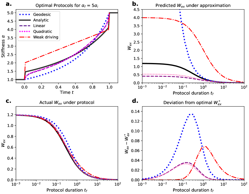
Figure 4: Comparison of different approximations. Solid black = true optimal protocol from [seifert2007], blue dotted = Sivak-Crooks geodesic optimal protocol [Eq. (70)], red dot-dash = Bonança-Deffner weak-driving optimal protocol [Eq. (69)], purple dashed = unconstrained linear response optimal protocol [Eq. (68)], pink dotted = unconstrained quadratic response optimal protocol [Eq. (73)]. All protocols are computed for a time discretization of 100 steps and a factor of 5 increase in the trap stiffness $\alpha_{f}=5\alpha_{i}$. a. Optimal protocols for $t_{f}=1$ according to the different approximations. b. For different protocol durations, the predicted excess work according to the approximations from Eqs. (68), (69), (72), and  (73). c. Actual excess work for optimal protocols suggested by each approximation at a given protocol durations, evaluated by numerically solving the Fokker-Planck equation. d. Deviation of the true excess work for approximated optimal protocols from exact optimal protocol, as evaluated by numerically solving the Fokker-Planck equation. Note the good performance of weak driving protocols for short times even for strong protocols (despite poor match between the approximated work as shown in panel 4.b.), the good performance of the slow-driving approximations for long times, and the modest improvement of quadratic response over linear response which peaks at a $\sim$$12\%$ decrease in the deviation from the analytically optimal excess work.

To evaluate the role of the next-order relaxation function, we can compute optimal protocols including only the linear relaxation function, and then compare with the optimal protocol including both the linear and quadratic relaxation functions. This can be done by directly optimizing our expression for the work, or by applying the additional weak driving or slow driving approximations.

To linear order, the excess work can be derived from the first term in the Volterra series. For the stiffening harmonic oscillator, with $\alpha(t_{f})=\alpha_{f},\,\alpha(0)=\alpha_{i}$, this can be written as

$$\langle W^{(1)}_{\mathrm{ex}}\rangle=\int^{t_{f}}_{0}{\mathrm{d}t}\,\dot{\alpha}(t)\int^{t}_{0}{\mathrm{d}t}_{1}\dot{\alpha}(t_{1})\Big[\frac{e^{-2\alpha(t)[t-t_{1}]}}{2\alpha^{2}(t)}\Big].$$ (68)

In the weak driving limit, we have

$$\langle W^{(1)}_{\mathrm{ex,\,weak}}\rangle=\int^{t_{f}}_{0}{\mathrm{d}t}\,\dot{\alpha}(t)\int^{t}_{0}{\mathrm{d}t}_{1}\dot{\alpha}(t_{1})\Big[\frac{e^{-2\alpha_{i}[t-t_{1}]}}{2\alpha_{i}^{2}}\Big].$$ (69)

Optimal protocols can be obtained numerically from each of these expressions by discretizing time and varying the control parameter at each point, as described in Appendix C.

Results from slow-driving thermodynamic geometry can be obtained by Taylor expanding the velocity as in Eq. (27).

$$\langle W^{(1)}_{\mathrm{ex,geo}}\rangle=\int^{t_{f}}_{0}{\mathrm{d}t}\,\dot{\alpha}^{2}(t)\Big[\frac{1}{4\alpha^{3}(t)}\Big],$$ (70)

from which the optimal $\alpha(t)$ can be derived analytically

$$\alpha_{\mathrm{geo}}(t)=\frac{t_{f}^{2}\alpha_{i}\alpha_{f}}{(t_{f}\sqrt{\alpha_{f}}\,-t[\sqrt{\alpha_{f}}+\sqrt{\alpha_{i}}])^{2}},$$ (71)

which gives us

$$\langle W^{(1)}_{\mathrm{ex,\,geo}}\rangle=\frac{(\sqrt{\alpha_{i}}-\sqrt{\alpha_{f}})^{2}}{t_{f}\alpha_{f}\alpha_{i}}.$$ (72)

To quadratic order, the excess work can be written as

$$\langle W^{(2)}_{\mathrm{ex}}\rangle=\int^{t_{f}}_{0}{\mathrm{d}t}\,\dot{\alpha}_{t}\int^{t}_{0}{\mathrm{d}t}_{1}\dot{\alpha}_{t_{1}}\Bigg\{\frac{e^{-2\alpha_{t}[t-t_{1}]}}{2\alpha_{t}^{2}}+\int^{t_{1}}_{0}{\mathrm{d}t}_{2}\dot{\alpha}_{t_{2}}\bigg[\frac{[1-\alpha_{t}(t_{2}-t_{1})]e^{-2\alpha_{t}(t-t_{1})}}{2\alpha_{t}^{3}}+\frac{[1-\alpha_{t}(t_{1}-t_{2})]e^{-2\alpha_{t}(t-t_{2})}}{2\alpha_{t}^{3}}\bigg]\Bigg\},$$ (73)

where we have used the notation $\alpha_{t}=\alpha(t)$ for space. Again the protocol is varied step by step to optimize this function.

Results from the optimization of these approximations are shown in Fig. 4. For the stiffening harmonic trap, we see that the inclusion of the quadratic correction leads to only a small change in shape of the resulting control protocol, as can be seen in Fig. 4.a in comparing the dashed purple (“Linear”) and dotted pink (“Quadratic”) curves, and only a marginal improvement in performance, as displayed in Fig. 4.d where at maximum we observe an improvement of $\sim$$12\%$ (for $\alpha_{f}=5\alpha_{i}$ at a time discretization of $100$ steps).

A significant computational cost accompanies the inclusion of the quadratic term, since optimizing Eq. (73) requires the evaluation of a more complex integral. The algorithm for evaluating the unrestricted linear work (as expressed Appendix C) for a given protocol has a time complexity $O(N^{2})$ while the quadratic work has a time complexity $O(N^{3})$, with $N$ being the step number in the discretized protocol. Empirically, we see that the ratio between the evaluation time for optimization of the protocol minimizing the linear work Eq. (68) and the evaluation time for optimization of the quadratic approximation Eq. (73) is $\sim$$9.1$ times longer for a $50$ step protocol, $\sim$$22$ times longer for a $100$ step protocol, $\sim$$36$ times longer for a $150$ step protocol (starting from a linear initial protocol for $t_{f}=1$, $\alpha_{f}=5\alpha_{i}$). The optimization of the quadratic approximation takes $\sim$$0.4s$ for $50$ steps, $\sim$$5.9s$ for $100$ steps, and $\sim$$56s$ for $150$ steps as evaluated on an Apple M4 processor.

IV Discussion

Here we have shown how various approximations commonly used in optimal stochastic thermodynamics relate to one another and can be derived from the general Volterra series expansion, and subsequently how higher-order response may be applied to optimal stochastic thermodynamics. Results from near-equilibrium thermodynamic geometry arise from adding a low-acceleration assumption to linear response, while weak-driving results are given by assuming the response of the system is equal to the system’s initial response. These approximations are valid for weak and slow driving regimes because higher orders of the Volterra series contribute only for higher orders of driving speed and perturbation strength.

The results for the harmonic oscillator demonstrate that while including the quadratic response can marginally improve performance, a computational cost is incurred from the evaluation of a computationally complex triple-integral. Further extension to higher orders beyond quadratic response with increasingly complex integrals to evaluate will correspondingly incur greater computational costs. Additionally, the inclusion of higher-order terms allows for the possibility of unphysical negative work and convergence issues for optimal protocols, as the cost function is no longer guaranteed to be positive or bounded from below. Exploring the contribution of quadratic and higher-order response to systems which are more nonlinear than the harmonic case would be an interesting avenue of future work, however, convergence issues may persist in these cases.

Similarly, as discussed in Appendix B, slow-driving perturbative expansions can be taken to higher orders, however, similar issues arise relating to the possibility of unphysical negative excess work, and convergence to true optimal protocols may be prevented by the divergence of the first term in the perturbative series for protocols with jumps.

These difficulties suggest a fundamental issue with relying on approximations that expand around $\rho^{\mathrm{eq}}_{\lambda}$ in the calculation of optimal protocols. We know that true optimal protocols include discontinuous jumps [seifert2007, zhong2024, aurell2011optimal, Aurell2012BoundaryLayers]. Since the nonequilibrium probability density $\rho_{t}$ will not instantaneously react to a change in the Hamiltonian, the approximation $\rho_{t}\approx\rho^{\mathrm{eq}}_{\lambda(t)}$ is fundamentally inapplicable for understand optimal protocols in region 3 of Fig. 1 (neither weak nor slow driving). As demonstrated here, attempting to extend near-equilibrium approximations can generate convergence issues and unphysical results while requiring increasingly complex calculations and added computational costs.

Recent results based on optimal transport circumvent this issue by considering the optimal evolution of the underlying density $\rho_{t}$ [zhong2024]. For overdamped dynamics, we know that in optimal processes the probability density $\rho_{t}$ follows the Wasserstein geodesic from optimal transport [ito2024geometric, aurell2011optimal, otto2001geometry, villani2021topics]: through integration by parts in both $x$ and $t$ (see [zhong2024] for details), the excess work [Eq. (9)] may be rewritten without an explicit $\dot{\lambda}$ dependence:

$$\langle W_{\mathrm{ex}}\rangle_{\Lambda}=\int_{0}^{t_{f}}\|\dot{\rho}_{t}\|^{2}_{{}_{\mathrm{OT}}}{\mathrm{d}t}+\beta^{-1}D_{\mathrm{KL}}(\rho_{t_{f}}|\rho^{\mathrm{eq}}_{\lambda_{f}}),$$ (74)

where $\|\dot{\rho}_{t}\|^{2}_{{}_{\mathrm{OT}}}$ is given by the Benamou-Brenier objective function [ito2024geometric, benamou2000computational], and $D_{\mathrm{KL}}(\rho_{A}|\rho_{B}):=\int\rho_{A}\ln(\rho_{A}/\rho_{B})\,{\mathrm{d}x}$ is the KL-divergence.

Intriguingly, if the solution to the Fokker-Planck equation [Eq. (3)] can be written as $\rho_{t}=\rho^{\mathrm{eq}}_{\gamma(t)}$ for a separate curve $\gamma(t)\in\mathcal{M}$, then the excess work can be expressed exactly with the friction tensor [Eq. (29)]

$$\langle W_{\mathrm{ex}}\rangle_{\Lambda}=\int_{0}^{t_{f}}\dot{\gamma}^{\mu}\dot{\gamma}^{\nu}\zeta_{\mu\nu}\big(\gamma(t)\big){\mathrm{d}t}+\beta^{-1}D_{\mathrm{KL}}(\rho^{\mathrm{eq}}_{\gamma(t_{f})}|\rho^{\mathrm{eq}}_{\lambda_{f}})$$ (75)

due to a recently discovered equivalence between thermodynamic geometry and optimal transport [zhong2024].

Rather than relying on expansions around $\rho^{\mathrm{eq}}_{\lambda}$, optimal protocols can be derived for any regime (all regions 0-3 in Fig. 1) by solving for a path $\gamma(t)\in\mathcal{M}$ that minimizes Eq. (75), and constructing the optimal protocol $\lambda(t)$ to ensure $\rho_{t}\approx\rho^{\mathrm{eq}}_{\gamma(t)}$ via counterdiabatic driving (e.g., [iram2021controlling]). This suggests that expansions around dynamically evolving reference densities, such as $\rho^{\mathrm{eq}}_{\gamma(t)}$ (c.f., [zhong2024, zhong2025optimal]), rather than instantaneous equilibrium states $\rho^{\mathrm{eq}}_{\lambda(t)}$, may be a more promising route for developing efficient optimal-control methods far from equilibrium.

V Acknowledgements

We would like to thank Neha Wadia, Hana Mir, and Steven Blaber for insightful conversations. S.D. was supported in part by an H2H8 research fellowship. A.Z. was supported by the Department of Defense (DoD) through the National Defense Science & Engineering Graduate (NDSEG) Fellowship Program. This research was supported by CoCoSys, one of the seven centers in JUMP 2.0, a Semiconductor Research Corporation (SRC) program sponsed by DARPA; in part by grants from the NSF (DMS-2235451) and Simons Foundation (MPS-NITMB-00005320) to the NSF-Simons National Institute for Theory and Mathematics in Biology (NITMB); as well as in part by the U.S. Army Research Laboratory and the U.S. Army Research Office under Contract No. W911NF-20-1-0151.

Appendix A Equivalence between Linear Response and Perturbative Slow-Driving Metrics

The perturbative [Wadia_2022] and linear response [sivak2012] slow-driving metrics can be shown to be equivalent using the spectral properties of the Fokker-Planck operator.

A.1 Perturbative friction tensor

Following [Wadia_2022], by plugging in the formal perturbative expansion $\rho_{t}=\rho^{\mathrm{eq}}_{\lambda(t)}+\delta\rho_{t}^{(1),P}+\delta\rho_{t}^{(2),P}+...$ into $\partial_{t}\rho_{t}=\mathcal{L}_{\lambda(t)}[\delta\rho_{t}]$ (Eq. (6)), one gets

$$\delta\rho_{t}^{(1),P}=\mathcal{L}_{\lambda(t)}^{-1}[\partial_{t}\rho^{\mathrm{eq}}_{\lambda(t)}],$$ (76)

and $\delta\rho_{t}^{(\ell+1),P}=\mathcal{L}_{\lambda(t)}^{-1}[\partial_{t}\delta\rho_{t}^{(\ell),P}]$, where $\mathcal{L}_{\lambda(t)}^{-1}$ is the inverse of the Fokker-Planck operator.

By defining and further manipulation

$$\langle W_{\mathrm{ex}}^{(1),P}\rangle =\int{\mathrm{d}t}\dot{\lambda}^{\mu}\int{\mathrm{d}x}\,\delta f_{\mu}\delta\rho_{t}^{(1),P}$$ (77)

$$=\int{\mathrm{d}t}\dot{\lambda}^{\mu}\int{\mathrm{d}x}\,\delta f_{\mu}\mathcal{L}_{\lambda(t)}^{-1}[\dot{\lambda}^{\nu}\delta f_{\nu}\rho^{\mathrm{eq}}_{\lambda(t)}]$$ (78)

$$=\int{\mathrm{d}t}\dot{\lambda}^{\mu}\dot{\lambda}^{\nu}\zeta^{P}_{\mu\nu}(\lambda(t)),$$ (79)

one arrives at the perturbative friction tensor (Eq. (72) in [wadia2022solution])

$$\zeta^{P}_{\mu\nu}(\lambda) =-\int{\mathrm{d}x}^{\prime}{\mathrm{d}x}^{\prime\prime}\Big(\rho^{\mathrm{eq}}_{\lambda}(x^{\prime\prime})\Big[\frac{\partial\ln\rho^{\mathrm{eq}}_{\lambda}(x^{\prime\prime})}{\partial\lambda^{\mu}}\Big]$$ (80)

$$G_{\lambda}(x^{\prime};x^{\prime\prime})\Big[\frac{\partial\ln\rho^{\mathrm{eq}}_{\lambda}(x^{\prime\prime})}{\partial\lambda^{\nu}}\Big]\Big),$$

where $G_{\lambda}(x,y)$ is the Green’s function of the Fokker-Planck operator $\mathcal{L}_{\lambda(t)}$. In terms of the eigenvectors of the Fokker-Planck operator [Eqns. (49) and (50)], this is

$$G_{\lambda}(x;y)=\sum_{n\geq 1}\frac{\rho_{r,n}(x)\rho_{l,n}(y)}{r_{n}}.$$ (81)

Recalling Eq. (2), note that $\partial\ln\rho^{\mathrm{eq}}_{\lambda}/\partial\lambda^{\mu}=f_{\mu}(x)-\langle f_{\mu}\rangle_{eq}=\delta f_{\mu}$, allowing us to rewrite Eq. (80) as

$$\zeta^{P}_{\mu\nu}(\lambda) =-\sum_{n\geq 1}\int{\mathrm{d}x}^{\prime}{\mathrm{d}x}^{\prime\prime}\Big(\rho^{\mathrm{eq}}_{\lambda}(x^{\prime\prime})\delta f_{\mu}(x^{\prime\prime})$$ (82)

$$\Big[\frac{\rho_{r,n}(x^{\prime})\rho_{l,n}(x^{\prime\prime})}{r_{n}}\Big]\delta f_{\nu}(x^{\prime\prime})\Big).$$

Since the $\rho_{l,n}$ form a complete basis, we can expand $f_{\mu}(x)$ as

$$f_{\mu}(x)=\sum_{m\geq 0}c_{\mu,m}\rho_{l,m}(x),$$ (83)

where $c_{\mu,m}=\int{\mathrm{d}x}f_{\mu}(x)\rho_{r,m}(x)$. Since $\delta f_{\mu}(x)=f_{\mu}(x)-\int{\mathrm{d}x}^{\prime}\rho_{r,0}(x^{\prime})f_{\mu}(x^{\prime})$, we see that

$$\delta f_{\mu}(x)=\sum_{m\geq 1}c_{\mu,m}\rho_{l,m}(x).$$ (84)

Expanding the conjugate forces in Eq. (82)), and applying the identity Eq. (53) to the integrals over $x^{\prime}$ and $x^{\prime\prime}$, we find

$$\zeta^{P}_{\mu\nu}(\lambda) =-\sum_{n\geq 1}\frac{c_{\mu,n}c_{\nu,n}}{r_{n}}.$$ (85)

A.2 Linear response friction tensor

Following [sawchuk2024dynamical], we note that the excess conjugate force correlation function $\Psi_{ab}^{(1)}(\lambda(t);\tau)=\langle\delta f_{a}(0)\delta f_{b}(\tau)\rangle^{\mathrm{eq}}_{\lambda(t)}.$ [Eq. (26)] can be written in terms of the probability $P(x^{\prime\prime},t^{\prime\prime},x^{\prime},0)$, of a particle which is at $x^{\prime}$ at $0$ and at $x^{\prime\prime}$ at $t^{\prime\prime}$

$$\zeta^{(1)}_{\mu\nu}(\lambda)=\int^{\infty}_{0}{\mathrm{d}t}^{\prime\prime}\int{\mathrm{d}x}^{\prime}{\mathrm{d}x}^{\prime\prime}\delta f_{\mu}(x^{\prime})\delta f_{\nu}(x^{\prime\prime})P(x^{\prime\prime},t^{\prime\prime},x^{\prime},0).$$ (86)

This probability can be expressed as

$$P(x^{\prime\prime},t^{\prime\prime},x^{\prime},0)=e^{\mathcal{L}t^{\prime\prime}}\delta(x^{\prime\prime}-x^{\prime})\rho^{\mathrm{eq}}_{\lambda}(x^{\prime}),$$ (87)

where $\mathcal{L}$ here acts on $x^{\prime\prime}$. Using the identity (52), we can rewrite this expression in terms of left and right eigenfunctions

$$P(x^{\prime\prime},t^{\prime\prime},x^{\prime},0) =\sum_{s\geq 0}\Big(e^{\mathcal{L}t^{\prime\prime}}\rho_{l,s}(x^{\prime})\rho_{r,s}(x^{\prime\prime})\Big)\rho^{\mathrm{eq}}_{\lambda}(x^{\prime})$$ (88)

$$=\sum_{s\geq 0}e^{r_{s}t^{\prime\prime}}\rho_{r,s}(x^{\prime})\rho_{r,s}(x^{\prime\prime}).$$

This gives us

$$\zeta^{(1)}_{\mu\nu}(\lambda) =\sum_{s\geq 0}\int^{\infty}_{0}{\mathrm{d}t}^{\prime\prime}e^{r_{s}t^{\prime\prime}}\int{\mathrm{d}x}^{\prime}{\mathrm{d}x}^{\prime\prime}\Big(\delta f_{\mu}(x^{\prime})\delta f_{\nu}(x^{\prime\prime})$$ (89)

$$\rho_{r,s}(x^{\prime})\rho_{r,s}(x^{\prime\prime})\Big).$$

We can now expand the conjugate forces again using Eq. (84), giving us

$$\zeta^{(1)}_{\mu\nu}(\lambda) =\sum_{s\geq 0}\sum_{n\geq 1}\sum_{m\geq 1}\int^{\infty}_{0}{\mathrm{d}t}^{\prime\prime}e^{r_{s}t^{\prime\prime}}c_{\mu,n}c_{\nu,m}$$ (90)

$$\int{\mathrm{d}x}^{\prime}{\mathrm{d}x}^{\prime\prime}\Big(\rho_{l,n}(x^{\prime})\rho_{l,m}(x^{\prime\prime})\rho_{r,s}(x^{\prime})\rho_{r,s}(x^{\prime\prime})\Big).$$

Using Eq. (53) and evaluating the integral over $t^{\prime\prime}$, we see that

$$\zeta^{(1)}_{\mu\nu}(\lambda) =-\sum_{n\geq 1}\frac{c_{\mu,n}c_{\nu,n}}{r_{n}}.$$ (91)

Comparing Eq. (85) and (91) we see the perturbative and linear response first-order friction tensors are equivalent.

Appendix B Higher-Order Perturbative Expansion for Moving Overdamped Harmonic Trap

We can assess the potential of the higher-order perturbative approach by focusing on the simple case of a moving harmonic trap of fixed stiffness. The perturbative expansion for the probability density can be written as

$$\rho(x;t)=\rho^{\mathrm{eq}}_{\lambda(t)}(x)+\int{\mathrm{d}x}^{\prime}G_{\lambda(t)}(x;x^{\prime})\frac{\partial}{\partial t}\rho_{\lambda(t)}^{\mathrm{eq}}(x^{\prime})$$ (92)

$$+\int{\mathrm{d}x}^{\prime\prime}G_{\lambda}(x;x^{\prime\prime})\frac{\partial}{\partial t}\int{\mathrm{d}x}^{\prime}G_{\lambda(t)}(x^{\prime\prime};x^{\prime})\frac{\partial}{\partial t}\rho^{\mathrm{eq}}_{\lambda(t)}(x^{\prime})+.$$

This expression can be simplified by writing it in terms of an integral operator

$$\hat{G}_{\lambda(t)}=\int dy\,G_{\lambda(t)}(x;y)=\int dy\,\sum_{n\geq 1}\frac{\rho_{r,n}(x)\rho_{l,n}(y)}{r_{n}}.$$ (93)

The $k^{th}$ term in the perturbative series can be written as follows, where $\rho^{(0)}_{\lambda(t)}(x)=\rho^{\mathrm{eq}}_{\lambda(t)}(x)$:

$$\rho^{(k)}_{\lambda(t)}(x)=\Big(\hat{G}_{\lambda(t)}\frac{d}{dt}\Big)^{k}\rho^{\mathrm{eq}}_{\lambda(t)}(x).$$ (94)

This defines a perturbative expansion for the work. By inserting Eq. (92) into the original definition of work, Eq. (1), where the power $\frac{d\langle W\rangle}{dt}=\sum_{k=0}\frac{d\langle W^{(k)}\rangle}{dt}$ (with $\frac{d\langle W_{\mathrm{ex}}\rangle}{dt}=\sum_{k=1}\frac{d\langle W^{(k)}\rangle}{dt}$ and $\frac{d\langle W_{\mathrm{rev}}\rangle}{dt}=\frac{d\langle W^{(0)}\rangle}{dt}$), we arrive at

$$\frac{d\langle W^{(k)}\rangle}{dt}=\int{\mathrm{d}x}\frac{dH_{\lambda(t)}(x)}{dt}\Big(\hat{G}_{\lambda(t)}\frac{d}{dt}\Big)^{k}\rho^{\mathrm{eq}}_{\lambda(t)}.$$ (95)

Here we assume the same potential as Eq. (54), giving us the same equilibrium distribution and left eigenfunction Eq. (49), but with $\alpha=1$:

$$V_{\mu(t)}(x)=\frac{[x-\mu(t)]^{2}}{2}.$$ (96)

We can then consider the successive application of the time-derivative and Green’s function integral operators to the equilibrium distribution to evaluate higher-order terms in the work expansion. To do so, let us first point out some important relationships. Recalling $\rho^{\mathrm{eq}}_{\lambda(t)}=e^{-H_{\lambda(t)}(x)}/Z$, for the moving harmonic oscillator with static stiffness, the partition function $Z$ is time independent

$$Z(t)=\int{\mathrm{d}x}\,e^{-[x-\mu(t)]^{2}/2}=\sqrt{2\pi}.$$ (97)

This observation simplifies further steps, which might otherwise be complex. The eigenfunctions are given by

$$\rho_{r,n}=\rho^{\mathrm{eq}}_{\mu(t)}\rho_{l,n}=\frac{1}{\sqrt{n!}}\text{He}_{n}(x-\mu(t))\rho^{\mathrm{eq}}_{\mu(t)},$$ (98)

which correspond to eigenvalues

$$r_{n}=-n.$$ (99)

Noticing $\dot{V}_{\lambda(t)}=dV_{\lambda(t)}/{\mathrm{d}t}=-\dot{\mu}[x-\mu]=\dot{\mu}\rho_{l,1}$, and $d\rho^{\mathrm{eq}}_{\mu(t)}/dt=-\dot{V}_{\mu(t)}\rho^{\mathrm{eq}}_{\mu(t)}=\dot{\mu}[x-\mu]\rho^{\mathrm{eq}}_{\mu(t)}=\dot{\mu}\rho_{r,1}$, we can evaluate the first term of the series

$$\frac{d\langle W^{(1)}\rangle}{dt}=\int{\mathrm{d}x}\,\dot{V}_{\mu(t)}\Big(\hat{G}_{\mu(t)}\frac{d}{dt}\Big)\rho^{\mathrm{eq}}_{\mu(t)}$$ (100)

$$=-\int{\mathrm{d}x}\,\dot{\mu}(t)\,\rho_{l,1}(x)\int dy\,\sum_{n\geq 1}\frac{\rho_{r,n}(x)\rho_{l,n}(y)}{r_{n}}\,\dot{\mu}(t)\,\rho_{r,1}(y).$$

Applying Eq. (53), we see that

$$\frac{d\langle W^{(1)}\rangle}{dt}=-\frac{\dot{\mu}^{2}(t)}{r_{1}}.$$ (101)

Higher-order terms can be evaluated by noticing that, by Eq. (53), only terms with $\rho_{r,1}$ will remain. We can derive a simple expression for this expansion to all orders by using the fact that the terms with $\rho_{r,n}$ for $n\geq 2$ vanish, by considering the application of the operator $\hat{G}_{\mu(t)}\frac{d}{dt}$ to the product of a function of $\mu$ and its derivatives, $\phi(\mu,\dot{\mu},\ddot{\mu},...)=\phi(t)$ with right eigenfunction $\rho_{r,k}$

$$\hat{G}_{\lambda(t)}\frac{d}{dt}\Big(\phi(t)\rho_{r,k}\Big)=\hat{G}_{\lambda(t)}\frac{d}{dt}\Big(\dot{\phi}(t)\rho_{r,k}$$ (102)

$$+\phi(t)\frac{-\dot{\mu}(t)\text{He}_{k}^{\prime}(x-\mu(t))}{\sqrt{k!}}\rho^{\mathrm{eq}}_{\mu(t)}$$

$$+\phi(t)\frac{\dot{\mu}(t)[x-\mu(t)]\text{He}_{k}(x-\mu(t))}{\sqrt{k!}}\rho^{\mathrm{eq}}_{\mu(t)}\Big).$$

Using the Hermite polynomial identity

$$\text{He}_{n+1}(x)=x\text{He}_{n}(x)-\text{He}_{n}^{\prime}(x),$$ (103)

Eq. (102) becomes

$$\hat{G}_{\lambda(t)}\frac{d}{dt}\Big(\phi(t)\rho_{r,k}\Big)=\frac{\dot{\phi}(t)}{r_{k}}\rho_{k,r}+\frac{\dot{\mu}(t)\phi(t)\sqrt{k+1}}{r_{k+1}}\rho_{k+1,r}.$$ (104)

The first order term in the series is proportional to $\rho_{r,1}$ as seen in the second line of Eq. (100). For second- and higher-order terms, only those that are proportional to $\rho_{r,1}$ remain, while all terms proportional to $\rho_{r,n}$ with $n>1$, vanish. This gives us the general expression for all orders:

$$\frac{d\langle W^{(k)}\rangle}{dt} =-\dot{\mu}(t)\Big(\frac{d}{dt}\Big)^{k}\frac{[\mu(t)]}{\prod^{k}_{i=1}r_{1}}$$ (105)

$$=-\dot{\mu}(t) \Big(\frac{d}{dt}\Big)^{k}\frac{\mu(t)}{(-1)^{k}}=-\dot{\mu}(t)\Big(-\frac{d}{dt}\Big)^{k}\mu(t).$$

giving us the work to an arbitrary expansion order $K$,

$$\langle W\rangle\approx\int_{0}^{t_{f}}{\mathrm{d}t}\,\Big[\sum^{K}_{k=0}-\dot{\mu}(t)\Big(-\frac{d}{dt}\Big)^{k}\mu(t)\Big].$$ (106)

The full expansion allows us to identify two issues arising from the inclusion of higher orders of the perturbative expansion. First, the even-$k$ higher orders will contribute negative work, meaning that if the series is truncated at a the $K$th order, the function $\mu(t)$ can be optimized to maximize odd orders and minimize even orders, allowing for the possibility of unphysical negative excess work. The work truncated at quadratic order $K=2$ can be written as

$$\langle W_{\mathrm{ex}}\rangle \approx\int_{0}^{t_{f}}{\mathrm{d}t}\,\Big(\frac{d\langle W^{(1)}\rangle}{dt}+\frac{d\langle W^{(2)}\rangle}{dt}\Big)$$ (107)

$$=\int^{t_{f}}_{0}{\mathrm{d}t}\,\Big(\dot{\mu}^{2}(t)-\dot{\mu}(t)\ddot{\mu}(t)\Big).$$

For even a simple protocol we can obtain a negative excess work:

$$\mu(t)=\begin{cases}0,&t<0,\\ \frac{t^{2}}{2},&0\leq t\leq t_{f},\\ \frac{t_{f}^{2}}{2},&t>t_{f}.\end{cases}$$ (108)

Plugging this into Eq. (107) and integrating we find

$$\langle W_{\mathrm{ex}}\rangle=t^{2}_{f}\Big(\frac{t_{f}}{3}-\frac{1}{2}\Big),$$ (109)

which is only non-negative for $t_{f}>3/2$. Unphysical negative excess work is recovered in the low $t_{f}$ weak and fast limit.

Second, we can see that relying on this series may prevent the recovery of optimal protocols since the first term in the series diverges for protocols with jumps, which are present for the moving harmonic trap and common in optimal protocols generally [seifert2007, zhong2024, aurell2011optimal, Aurell2012BoundaryLayers]. The true optimal protocol for a moving harmonic trap starting at $\mu_{i}=0$ is

$$\mu^{*}(t)=\begin{cases}0,&t<0,\\[10.0pt] \dfrac{\mu_{f}(t+1)}{t_{f}+2},&0\leq t\leq t_{f},\\[6.0pt] \mu_{f},&t\geq t_{f},\end{cases}$$ (110)

which exhibits jumps of size $\mu_{f}/(t_{f}+2)$ at its endpoints [seifert2007]. This gives us the optimal velocity

$$\dot{\mu}^{*}(t)=\frac{\mu_{f}}{t_{f}+2}\cdot\bigg[\delta(t)+(\Theta(t)-\Theta(t-t_{f}))+\delta(t-t_{f})\bigg].$$ (111)

Integrating over $(\dot{\mu}^{*})^{2}$ is simplified by evaluating the $\delta$ and $\Theta$ functions, which appear with different time arguments. The first order of excess work is (with $0^{-}$ and $t_{f}^{+}$ specifying that the integral is taken over the entirety of the delta functions)

$$\langle W^{(1)}\rangle=\int^{t_{f}^{+}}_{0^{-}}dt\,\frac{\mu_{f}^{2}}{(t_{f}+2)^{2}}\bigg[\delta^{2}(t)+1+\delta^{2}(t-t_{f})\bigg].$$ (112)

We can investigate this expression by representing the Dirac delta function as a normal distribution of width $\epsilon$,

$$\delta(t)=\lim_{\epsilon\rightarrow 0}\frac{1}{\sqrt{2\pi}\epsilon}\exp\bigg[-\frac{t^{2}}{2\epsilon^{2}}\bigg].$$ (113)

Inserting this into Eq. (112), we find that for the optimal protocol, the first term in the series is divergent:

$$\langle W^{(1)}\rangle =\frac{\mu_{f}^{2}}{(t_{f}+2)^{2}}\bigg[t_{f}+\lim_{\epsilon\rightarrow 0}\int^{\infty}_{-\infty}dt\,\bigg[\frac{e^{-t^{2}/\epsilon^{2}}}{2\pi\epsilon^{2}}+\frac{e^{-(t-t_{f})^{2}/\epsilon^{2}}}{2\pi\epsilon^{2}}\bigg]$$ (114)

$$=\frac{\mu_{f}^{2}}{(t_{f}+2)^{2}}\bigg[t_{f}+\lim_{\epsilon\rightarrow 0}\frac{1}{\sqrt{\pi\epsilon}}\bigg]=\infty.$$

Because of this issue, we should not expect this series to converge to true optimal protocols, which are often functions with discontinuities. To avoid this, an interesting future direction may be the study of how regularization procedures as used elsewhere in physics can be applied to this case.

Appendix C Numerical Optimization and Work Evaluation

To numerically optimize the expressions in Section III, protocols were discretized in time to 100 evenly spaced points between $t=0$ and $t=t_{f}$ and optimized by varying the position of each of these 50 points. Protocols are initialized as linear between initial and final control parameters. Integrals were evaluated as discrete sums using the left hand rule, corresponding to an Itô interpretation of the stochastic dynamics. To approximate the excess work to linear order Eq. (68) becomes (with $N=50$, $\delta t=t_{f}/N$)

$$\langle W^{(1)}_{\mathrm{ex}}\rangle\approx\sum^{N-1}_{n=0}\delta t\frac{\alpha_{n+1}-\alpha_{n}}{\delta t}\sum^{n}_{m=0}\delta t\frac{\alpha_{m+1}-\alpha_{m}}{\delta t}\frac{e^{-\alpha_{n}(n-m)\delta t}}{2\alpha^{2}_{n}}.$$ (115)

For the weak driving limit, we set $\alpha_{n}$ in the response function to $\alpha_{0}$, so that the left hand side of Eq. (69) could be approximated as

$$\langle W^{(1)}_{\mathrm{ex,weak}}\rangle\approx$$ (116)

$$\sum^{N-1}_{n=0}\delta t\frac{\alpha_{n+1}-\alpha_{n}}{\delta t}\sum^{n}_{m=0}\delta t\frac{\alpha_{m+1}-\alpha_{m}}{\delta t}\frac{e^{-\alpha_{0}(n-m)\delta t}}{2\alpha^{2}_{0}}.$$

Approximating the excess work to quadratic order, Eq. (73) becomes

$$\langle W^{(1)}_{\mathrm{ex}}\rangle \approx\sum^{N-1}_{n=0}\delta t\frac{\alpha_{n+1}-\alpha_{n}}{\delta t}\sum^{n}_{m=0}\delta t\frac{\alpha_{m+1}-\alpha_{m}}{\delta t}\bigg[\frac{e^{-\alpha_{n}(n-m)\delta t}}{2\alpha^{2}_{n}}+\sum_{k=0}^{m}\delta t\frac{\alpha_{k+1}-\alpha_{k}}{\delta t}\frac{(1-\alpha_{n}(m-k)\delta t)\cdot e^{-\alpha_{n}(n-k)\delta t}}{2\alpha^{3}_{n}}\bigg].$$ (117)

In order to properly discretize these multi-dimensional integrals, care must be taken to compute the accessible volume within individual bins that straddle the boundary defined by limits of integration. Accordingly, terms for which either $n=m$ or $m=k$, without all three being equal, are multiplied by a factor of $1/2$, while terms for which $n=m=k$ are multiplied by a factor of $1/6$. Each of these expressions is minimized by varying $[\alpha_{0},\alpha_{1},...,\alpha_{N-1}]$, starting from a linear protocol. The optimal protocol for a given approximation is determined by minimizing Eqns. (115), (116), and (117) using scipy.optimize.minimize [2020SciPy-NMeth] according to the corresponding assumptions.

For each of these approximations, we compared the values given by optimizing them with the true values for the work, which we found by solving the Fokker-Planck equation numerically via the discretization in [holubec2019physically, zhong2022limited]. For this, protocols optimized according to the above approximations were fed into a Fokker-Planck simulation with a lattice-discretized state space with spacing $\Delta x=0.1$ from $x=-5$ to $x=5$. Code found at: https://github.com/SamuelDAmbrosia/Higher-order-stochastic-thermo .