Optimal Carbon Prices in an Unequal World:
The Role of Regional Welfare Weights

How should nations price carbon? This paper examines how the treatment of global inequality, captured by regional welfare weights, affects optimal carbon prices. I develop theory to identify the conditions under which accounting for differences in marginal utilities of consumption across countries leads to more stringent global climate policy in the absence of international transfers. I further establish a connection between the optimal uniform carbon prices implied by different welfare weights and heterogeneous regional preferences over climate policy stringency. In calibrated simulations, I find that accounting for global inequality reduces optimal global emissions relative to an inequality-insensitive benchmark. This holds both when carbon prices are regionally differentiated, with emissions 21% lower, and when they are constrained to be globally uniform, with the uniform carbon price 15% higher.

Keywords: carbon pricing, climate policy, global inequality, welfare weights, social welfare function.

JEL Codes: Q54, H23, D63, Q58.

1 Introduction

The distributional effects of climate change and climate policies are at the heart of international climate change negotiations. Central to these debates are inequalities in climate impacts, responsibilities for emissions, and capabilities to mitigate and adapt—aspects that are all interlinked with global wealth inequality [undefu]. These inequalities are recognized in international climate agreements, as exemplified by the principle of “common but differentiated responsibilities and respective capabilities” of the United Nations Framework Convention on Climate Change [undefaaae]. The Paris Agreement further emphasizes that developed countries should take the lead in reducing emissions, stressing equity considerations [undefaaaf].

Despite the importance of inequalities in international climate policy, the standard approach to estimating optimal carbon prices concentrates solely on efficiency and effectively disregards global inequality [undefaaf, undefaaan]. It does so by maximizing a social welfare function (SWF) with Negishi welfare weights, which are higher for wealthier countries, offsetting differences in marginal utilities of consumption across countries. In contrast, an alternative approach focuses on maximizing global welfare, subject to constraints on international transfers [undefr]. A common version of this approach maximizes the utilitarian SWF, which assigns equal weight to the welfare of all individuals. Crucially, the utilitarian SWF accounts for global inequality in that it considers differences in marginal utilities of consumption across wealthier and poorer countries. These differences in welfare weights may be particularly important, as the costs and benefits of emission reductions are unevenly distributed, with poorer countries often disproportionately impacted by climate change [undefs, undeft, undefat, undefaac]. Given that optimal carbon prices are well-known to be highly sensitive to the utility discount rate [undefaaac, undefaak]—a form of temporal welfare weighting—it may be surprising that comparatively little research has explored the role of regional welfare weights.

In this paper, I examine how the stance on global inequality—reflected in the choice of regional welfare weights—affects optimal carbon prices. I study this question theoretically, to uncover insights into the underlying economic forces, and through numerical simulations with the integrated assessment model RICE [undefaaf], to evaluate the quantitative implications for climate policy.

Specifically, I compare optimal carbon prices under the Negishi-weighted SWF to those under the utilitarian SWF, in the absence of international transfers. I begin by imposing the same two constraints on the utilitarian optimization that are implicit in the Negishi solution: no international transfers and uniform carbon prices. This constrains the utilitarian problem to an identical policy instrument—a globally uniform carbon price in each period—enabling a direct comparison with the Negishi solution. Next, I remove the uniform carbon price constraint, allowing for differentiated carbon prices, which can improve utilitarian welfare by shifting some of the abatement cost burden from poorer to wealthier countries. I refer to carbon prices in the utilitarian solution as welfare-maximizing carbon prices to highlight that they maximize the (unweighted or equally-weighted) sum of individuals’ utilities.

Using a theoretical model, I show that optimal carbon prices and aggregate abatement may be higher or lower in the utilitarian solutions than in the Negishi solution and that this depends on the distribution of the marginal climate damages and the abatement cost burden across countries. Specifically, the utilitarian climate policy is more stringent if poorer nations have comparatively high marginal climate damages and a relatively steep marginal abatement cost function, resulting in smaller changes in abatement when carbon prices are altered. In a dynamic extension of the model, I show that regional differences in population growth and economic growth critically influence how regional welfare weights affect optimal carbon prices by impacting the relative importance that regions place on the future, when most climate impacts occur, versus the present, when abatement efforts take place. Moreover, I establish a novel and intuitive connection between the uniform carbon prices under utilitarian and Negishi weights and nations’ preferred uniform carbon prices that maximize national welfare, a notion that was established by [undefaaah] and [undefaw]: The utilitarian uniform carbon price exceeds the Negishi-weighted carbon price if and only if poorer nations prefer higher uniform carbon prices than wealthier nations. At a conceptual level, I introduce the concept of welfare-cost-effectiveness, which refers to emission reductions that are achieved at the lowest possible welfare (utility) cost, contrasting it with the prevalent concept of cost-effectiveness, which focuses on minimizing monetary costs. I demonstrate that regionally differentiated utilitarian carbon prices are welfare-cost-effective, yielding higher carbon prices in wealthier countries, while Negishi-weighted carbon prices are cost-effective.

To address the theoretical ambiguity regarding whether accounting for inequality raises or lowers optimal carbon prices, I employ numerical simulations with RICE to explore the direction and magnitude of this effect. I find that the welfare-maximizing solutions yield more stringent climate policies than the Negishi solution. Simply put, accounting for inequality means stronger climate action. Specifically, the utilitarian uniform carbon price in 2025 is around 15% higher than the Negishi-weighted carbon price, under default discounting parameters. The utilitarian solution that allows for differentiated carbon prices features higher carbon prices in rich countries and lower carbon prices in poor countries; globally, cumulative emissions are 21% lower compared to the Negishi solution.

I leverage the theoretical insights to uncover the key drivers of the numerical results. The utilitarian differentiated carbon price solution results in reduced global emissions because the additional abatement in developed countries outweighs the reduced abatement in the poorest regions. Higher uniform carbon prices in the utilitarian solution, compared to the Negishi solution, are primarily driven by the poorest region, Africa, which is most impacted by climate change for two main reasons: it has the highest marginal damages and the fastest population growth. Using the theoretical link to regions’ preferred uniform carbon prices to strengthen the intuition, I find that Africa also favors the highest uniform carbon price—more than twice the preferred price of the US and the Negishi-weighted carbon price. Thus, the main intuition for lower carbon prices in the Negishi solution is as follows: by assigning lower weight to the welfare of poorer regions, Negishi weights effectively also downweight the region most impacted by climate change, leading to less stringent climate policy.

This paper makes several contributions to the literature on optimal carbon prices with heterogeneous regions. First, it provides a set of novel theoretical results on how optimal carbon prices depend on regional welfare weights. To my knowledge, it is the first paper to derive the conditions under which accounting for global inequality increases the optimal global climate policy stringency in the absence of transfers. In doing so, I identify factors that have previously been underappreciated in this context: regional heterogeneities in the convexity of the abatement cost function, population growth, and economic growth. These results build on influential papers by [undefw] and [undefaj], which show that globally uniform carbon prices are optimal if and only if distributional issues are ignored (through the choice of welfare weights) or unrestricted lump-sum transfers can be made between countries. I also offer a new perspective to the literature on regions’ preferred uniform carbon prices [undefaaah, undefaw]. Instead of focusing on voting mechanisms, I explore an aggregation of preferences rooted in welfare-economic theory. A related strand of literature explored aspects of efficiency and equity in emission permit markets [undefx, undefaay, undefaau, undefm]. In contrast, this paper focuses on a setting without international permit markets. Other related papers examined the importance of accounting for inequalities at a fine-grained level [undefad, undefaav], and how optimal carbon taxes, under different welfare weights, depend on distortionary fiscal policy [undefi, undefaa, undefai] and inequality within and between countries [undefav]. However, unlike the present paper, these studies do not theoretically explore how utilitarian and Negishi weights shape the optimal stringency of climate policy.

Second, this paper adds to a body of work that numerically investigates the role of regional welfare weights in IAMs. The study most closely related to this research is [undefb], which also compares the Negishi solution to a utilitarian solution, although using a different integrated assessment model. The present paper expands upon this study in multiple ways. First, it offers a deeper understanding of the key drivers behind the results by linking the new theoretical insights to the numerical findings and regional characteristics. Furthermore, I extend the analysis by examining the distributional implications, the utilitarian uniform carbon price, and regions’ preferred uniform carbon prices. This offers additional insights into heterogeneous climate policy preferences and further strengthens the intuition behind the numerical results. A related but distinct literature estimates the equity-weighted social cost of carbon (SCC), a measure of the marginal damages of carbon emissions that places more weight on the costs and benefits in poor countries. The key difference between this literature and the present paper is that the equity-weighted SCC typically estimates the marginal damages along non-optimal emissions pathways [undefh, undeff, undefa, undefd, undefaan], while this paper investigates how regional welfare weights affect optimal carbon prices.

The remainder of this paper is organized as follows. Section 2 provides conceptual background on the different optimization approaches. In Section 3, a theoretical model is introduced and key analytical results are derived. Section 4 describes modifications to the RICE model and presents simulation results. Section 5 concludes.

2 Conceptual Background

This section provides conceptual background on different optimization approaches in order to lay the foundation for my own analysis. In Section 2.1, the difference between positive and normative approaches is introduced. Section 2.2 discusses the positive approach. Finally, Section 2.3 provides a welfare-economic conceptualization of normative optimizations.

2.1 Positive and normative optimizations

The purpose of optimization is a main source of debate in climate economics, and two approaches are sometimes distinguished: positive and normative optimizations [undefau]. [undefaah, p. 1081] provides an instructive discussion of these two approaches, noting that “the use of optimization can be interpreted in two ways: they can be seen both, from a positive point of view, as a means of simulating the behavior of a system of competitive markets and, from a normative point of view, as a possible approach to comparing the impact of alternative paths or policies on economic welfare”. In brief, the positive approach seeks to identify the competitive equilibrium, while the normative approach aims at maximizing social welfare. Which approach is taken depends on the welfare weights in the SWF.

The issue of discounting, which determines the intertemporal weighting of consumption and welfare, has received much attention in the debate on positive versus normative optimization approaches [undefg, undefh, undefj, undefab, undefah, undefao, undefaak]. Under the positive approach, the discount rate is determined based on market observations. In contrast, the normative approach relies on ethical reasoning to determine the discount rate.

However, the difference between positive and normative optimization approaches extends to the interregional weighting of welfare. The typical positive approach relies on Negishi welfare weights, which are higher for rich individuals, to identify the competitive equilibrium. In contrast, under the normative approach, uniform welfare weights, which are also called utilitarian welfare weights, are most commonly used, weighting everybody’s welfare within a time period equally. This paper focuses on interregional welfare weights and how they influence optimal carbon prices.

While the distinction between positive and normative optimizations is useful to clarify the different purposes of optimization, this distinction is not always clear-cut in climate economics. In particular, it has been questioned whether it is possible to interpret the modeling choices that are typically made under the positive optimization approach as purely positive (see [undefv], for a discussion). Keeping this caveat in mind, I use the labels “positive” and “normative” to highlight the conceptual difference underlying these optimization approaches: whether the optimization seeks to simulate markets or to maximize social welfare.

2.2 The positive approach: Background on Negishi weights

Negishi welfare weights are commonly used in regionally disaggregated integrated assessment models of climate change. Popular IAMs that use Negishi weights include RICE [undefaaj], which this paper focuses on, MERGE [undefaaa], REMIND [undefax] and WITCH [undefn]. This section outlines the rationale for and critiques of using Negishi weights in IAMs. It finishes with a welfare economics perspective on the positive optimization approach.

2.2.1 Rationale for using Negishi weights in IAMs

The theoretical basis for the use of Negishi weights is a theorem by [undefaae]. Negishi proved that a competitive equilibrium can be found by maximizing a social welfare function in which the welfare of each agent is appropriately weighted such that each agent’s budget constraint is satisfied at the equilibrium [undefaaj]. The Negishi-weighted SWF is given by a weighted sum of agents’ utilities, where the weights are inversely proportional to the marginal utility of consumption. For identical and concave utility functions, which are commonly assumed, this implies higher welfare weights for wealthy individuals, with a low marginal utility of consumption, than for poorer individuals. The appeal of the Negishi-weighted SWF is that it provides a computationally convenient method to identify the competitive equilibrium, which is Pareto efficient if the conditions of the first fundamental theorem of welfare economics are satisfied.

Besides this theoretical foundation, there were two additional motivations for the use of Negishi weights in IAMs: (1) to prevent transfers across regions, which were considered politically infeasible or unrealistic [undefaaj], and (2) to obtain a uniform carbon price in all regions, ensuring that global emissions are reduced at the lowest possible cost. Indeed, to achieve these two objectives in every period of the RICE model, [undefaaj] made refinements to what they call the “pure Negishi solution” that relies on time-invariant welfare weights. Specifically, [undefaaj] adjust the Negishi weights in each time period such that the weighted marginal utility of consumption is equalized in each period [undefaaz]. This approach yields time-variant Negishi weights and accomplishes the goal of equalizing the carbon price across regions in every period. Moreover, these weights ensure that no cross-regional transfers take place, since such transfers do not increase the objective value of the Negishi-weighted SWF. Notably, without Negishi weights, social welfare could be increased by redistributing capital or consumption from rich to poor regions in models that maximize the unweighted sum of agents’ utilities, as long as utility is an increasing concave function of consumption, which is commonly assumed. Hence, the constraints of equalized carbon prices and no transfers are effectively incorporated in the time-variant Negishi weights used in RICE.

2.2.2 Critiques of using Negishi weights in IAMs

While Negishi weights are commonly used in IAMs, the use of such weights has been criticized on both ethical and theoretical grounds [undefc, undefaf, undefaaz, undefaaaa]. This section provides a summary of main critiques.

From an ethical perspective, a main critique is that Negishi weights assign greater weight to the welfare of people in rich countries than in poor countries. This is the case because Negishi weights are inversely proportional to the marginal utility of consumption and the utility function is typically assumed to be concave. Models with Negishi weights are thus “acting as if human welfare is more valuable in the richer parts of the world” [undefaaaa, 176]. Moreover, because Negishi weights equalize the weighted marginal utility of consumption, aspects of interregional equity are effectively ignored and global inequality is neglected [undefaaz, undefaaaa]. As a result, it is irrelevant whether poor or rich countries are affected by climate change and climate policies [undefad].

Moreover, [undefaaz] notes that models with Negishi weights have an inherent conceptual inconsistency: the diminishing marginal utility of consumption is embraced intertemporally, but suppressed interregionally. Consequently, transfers from richer to poorer individuals are desired in an intertemporal context but rejected in an interregional context.

Another criticism from a theoretical perspective is provided by [undefaf] and [undefc]. In a simple analytical model, these authors show that the time-variant Negishi weights, used for example in the RICE model [undefaaj], distort the time-preferences of agents and result in different saving rates than those implied by the underlying preference parameters. Furthermore, they note that the time-invariant weights proposed by [undefaae] do not have this problem because they only consist of one weight per agent, and thus only affect the distribution between agents, but leave the intertemporal choices of each agent unaffected.

A final criticism of Negishi weights concerns the manner in which Negishi weights are often introduced—if discussed at all—which is frequently rather technical with no or little transparent discussion of the ethical implications [undef, undefaaz].

2.2.3 Welfare economics perspective on the positive approach

This section provides a discussion of the positive optimization approach from the perspective of welfare economics. From the first fundamental theorem of welfare economics, it is known that, under certain conditions, the competitive equilibrium is Pareto efficient [undefaax]. The maximization of a Negishi-weighted SWF in IAMs seeks to identify the competitive equilibrium with a Pareto efficient level of abatement. I refer to this solution as the “Negishi solution”. The Negishi solution is one particular point—among infinitely many points—on the Pareto frontier in a first-best setting in which only resource and technology constraints are present (assuming that the conditions of the first fundamental theorem of welfare economics hold). Notably, it is the only Pareto efficient allocation in a first-best setting that does not require transfers [undefaay]. In the absence of abatement, the competitive equilibrium is not efficient due to the climate externality. The Pareto efficiency of the Negishi solution, and the inefficiency of no abatement, is illustrated in Figure 1a, which shows the Pareto frontier for a simple example with two regions: a rich Global North, and a comparatively poor Global South.

While the Negishi solution is Pareto efficient, it cannot generally be interpreted as maximizing social welfare in a normative sense. The Negishi-weighted SWF is not intended to reflect ethical theories of social welfare but is instead calibrated to support a Pareto-efficient allocation without requiring transfers. In contrast, normative analyses rely on social welfare functions grounded in explicit normative theories of social welfare. The most commonly used such theory in public economics is utilitarianism [undefam], which assigns equal weight to the welfare of all individuals. Importantly, the Negishi solution does not maximize aggregate welfare if the welfare of all people is weighted equally. Maximizing a utilitarian SWF maximizes the (equally-weighted) sum of the welfare of all individuals. This is illustrated in Figure 1b, which shows the social indifference curves of the utilitarian and Negishi-weighted SWFs, and the points that maximize these SWFs.

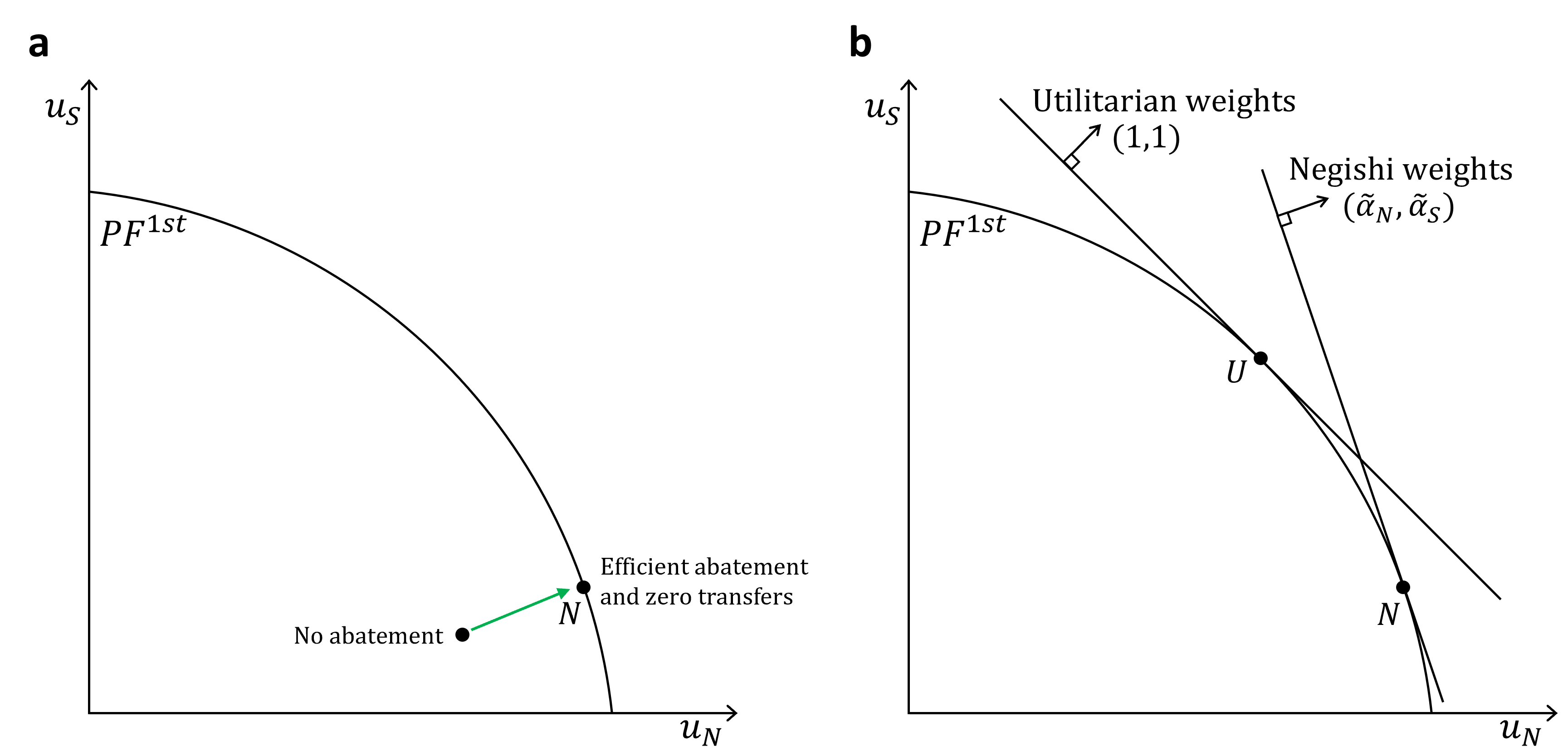
Figure 1: Illustrative two-region example of the welfare outcomes under the Negishi and utilitarian solutions.

Notes: Panel (a) shows that the Negishi solution ($N$) is Pareto efficient. Panel (b) shows an illustrative comparison of the Negishi ($N$) and utilitarian ($U$) solutions. The utilities of representative agents in the Global North and Global South are denoted by $u_{N}$ and $u_{S}$, respectively. $PF^{1st}$ is the Pareto frontier in a first-best setting. The welfare weights vectors are the gradient vectors of the SWFs, which are perpendicular to the linear social indifference curves. The Negishi weights are denoted by $\tilde{\alpha}_{i}$.

Given that the Negishi solution does not maximize aggregate (unweighted) welfare, how may the use of Negishi weights in IAMs be justified? There are at least two possible lines of argument. First, it may be argued that the Negishi solution has no normative but only a positive interpretation; that it is merely a procedure to identify the competitive equilibrium with Pareto efficient abatement and zero transfers. For example, [undefaah, 1111] notes that “if the distribution of endowments across individuals, nations, or time is ethically unacceptable, then the “maximization” is purely algorithmic and has no compelling normative properties”. Moreover, [undefaai, 20] clarify: “We do not view the solution as one in which a world central planner is allocating resources in an optimal fashion”.

A second line of argument used to support employing Negishi weights relies on the second fundamental theorem of welfare economics, which states that any point on the Pareto frontier can be supported as a competitive equilibrium if unrestricted lump-sum transfers can be made. This is sometimes used to argue that the issues of equity and efficiency can be separated. However, this typically is not the case for climate policy; the Pareto efficient abatement level generally depends on the distribution of wealth. This is because the marginal willingness to pay for abatement generally varies with income [undefaay]. Therefore, the Negishi solution only identifies a Pareto efficient abatement level if no transfers occur. Moreover, the practical relevance of the second welfare theorem has been questioned. For instance, [undefaax, 12] notes that “if there is an absence of—or reluctance to use—a political mechanism that would actually redistribute resource-ownership and endowments appropriately, then the practical relevance of the converse theorem [the second welfare theorem] is severely limited”.

To summarize, the abatement in the Negishi solution generally differs from the abatement that maximizes global utilitarian welfare (hereafter, simply “global welfare”), regardless of whether unrestricted transfers are feasible.

2.3 The normative approach: Welfare-economic conceptualization

This section provides a conceptualization of the normative optimization approach, grounded in welfare economics. In doing so, the objective of this section is to clarify the fundamental distinction between positive and normative optimization approaches in climate economics. In Section 2.2.1, I have argued that constraints are implicitly incorporated in the welfare weights under the positive approach. Here, I emphasize that this marks a key difference from the normative approach, where constraints and welfare weights are determined separately.

I propose to conceptualize the normative optimization approach as consisting of two steps. First, the social welfare function is defined based on ethical principles. Second, potential constraints are specified which affect the feasible set of allocations. The first step—the specification of the SWF based on ethical principles—is common in normative analyses. Such SWFs have a long tradition in public economics, and particularly in the optimal income taxation literature [undefaad, undefaam, undefam]. They are referred to as Bergson-Samuelson SWFs [undefk, undefaat] and produce an ethical ordering of societal outcomes. Common Bergson-Samuelson SWFs include the utilitarian, prioritarian and Rawlsian SWFs [undefaab]. In this paper, I focus on the utilitarian SWF, the most widely used normatively grounded Bergson-Samuelson SWF in climate economics.

The second step is to carefully consider and explicitly account for real-world constraints in the optimization. This step is often less thoroughly addressed in the existing literature. It is of course challenging to determine and formalize plausible real-world constraints, especially in stylized IAMs. It therefore seems valuable to explore a plausible range of constraints. Conceptually, such constraints affect the feasible set of allocations, which, in turn, determines the utility possibility set (UPS), which was introduced by [undefaat]. Ultimately, we are interested in the Pareto frontier, which is defined as the upper frontier of the UPS. Finally, the social optimum is the point on the Pareto frontier that maximizes the SWF.

Depending on the constraints imposed on the optimization, a conceptual distinction between first-best and second-best settings is frequently made [undefaab]. Typically, a first-best setting is considered to be a setting in which only resource and technology constraints are present, but otherwise the social planner has access to any policy instrument, including unrestricted lump-sum transfers. In contrast, the notion of second-best settings is used when additional constraints are present.

It is instructive to illustrate how the normative optimization approach works in the context of this paper. This is shown in Figure 2 for optimization problems considered in this paper. In the first step, the utilitarian SWF is specified (which has linear social indifference curves with slope -1). In the second step, potential constraints are specified. Of particular relevance in the context of international climate policy are constraints on international transfers and whether carbon prices are constrained to be uniform across countries.

In the first-best setting, there are no constraints apart from the usual resource and technology constraints. In particular, unrestricted lump-sum transfers can be made. In this setting, the social planner uses cost-effective and efficient uniform carbon prices to internalize the climate externality and lump-sum transfers to address distributional issues. With identical and concave utility functions, large transfers are made to equalize per capita consumption across regions [undefad], eliminating inequality. This results in the highest utilitarian welfare; the outermost social indifference curve, $W_{1st}$, is achieved.

However, as discussed above, such a first-best setting with large international transfers may be politically infeasible. As [undefaay, 43] puts it, “Unrestricted lump-sum transfers are a useful construct which scarcely exist outside the confines of economic theory”. As discussed in Section 2.2.1, the political infeasibility of large transfers was one of the reasons that motivated the use of Negishi weights under the positive optimization approach. In contrast, under the normative optimization approach, political transfer constraints affect the feasible set of allocations while welfare weights remain unchanged.

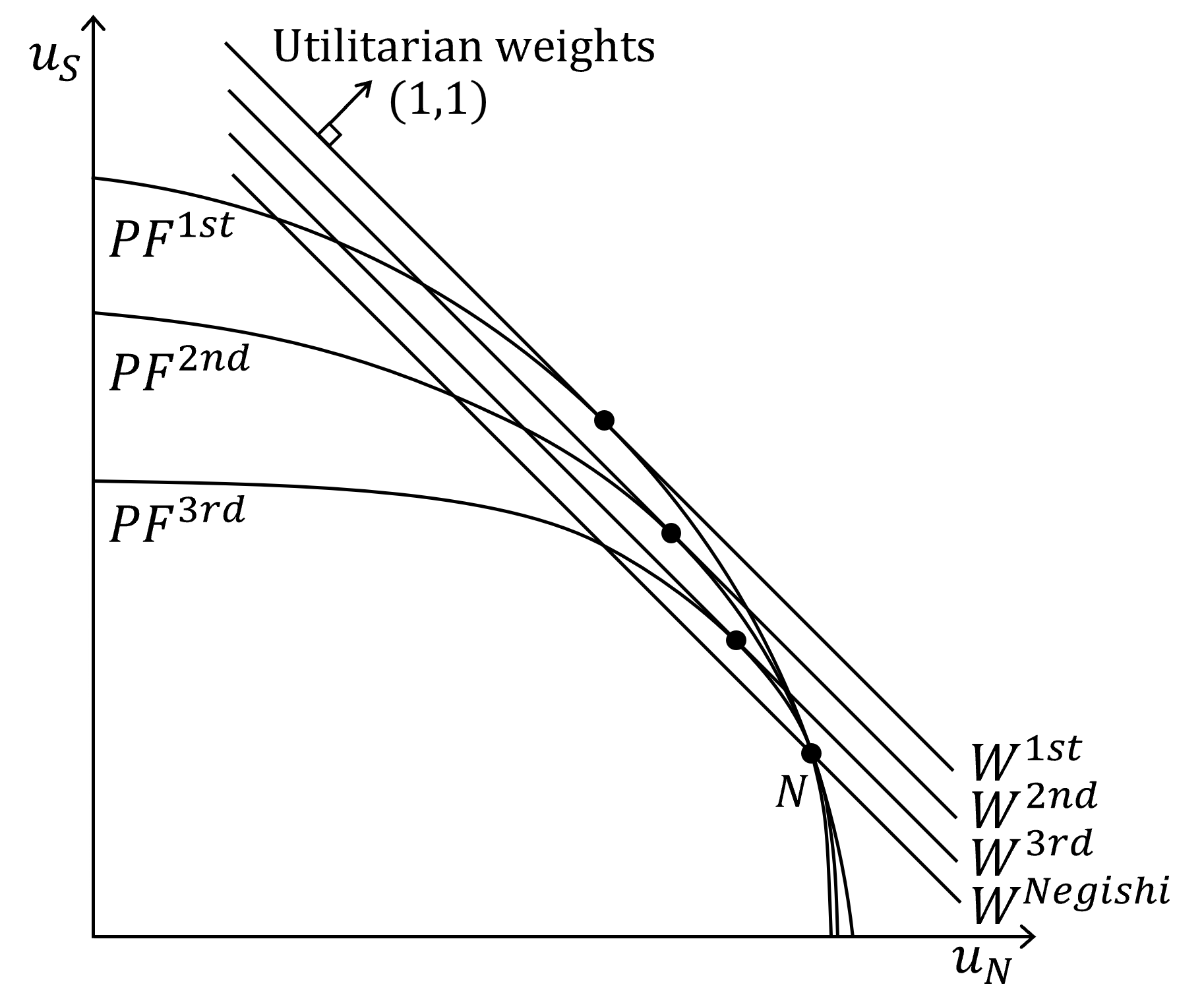
Figure 2: Illustration of the utilitarian social welfare outcomes in first-, second-, and third-best settings, and the Negishi solution.

Notes: The figure shows the utilitarian optima in first-, second-, and third-best settings and the utilitarian welfare level of the Negishi solution. The utilities of representative agents in the Global North and Global South are denoted by $u_{N}$ and $u_{S}$, respectively. $PF^{x}$ is the Pareto frontier in the $x^{th}$-best setting. $W^{x}$ is the utilitarian social indifference curve that corresponds to the social optimum in the $x^{th}$-best setting or the Negishi solution. The utilitarian weights vector is the gradient vector of the utilitarian SWF.

Let us now consider such a second-best setting in which international lump-sum transfers are infeasible. The lack of this policy option reduces the feasible set of allocations, the UPS gets smaller, and the Pareto frontier moves inward (except for one point on the frontier, which corresponds to the Negishi solution, which does not require transfers). Consequently, the social optimum lies on a lower social indifference curve, $W_{2nd}$. In the absence of the option to address inequality with lump-sum transfers, the utilitarian social planner accounts for global inequality in the climate policy design. Specifically, differentiated carbon prices that are higher in rich regions and lower in poor regions are used to reduce the welfare cost of abating emissions [undefw] (also see Section 3.2). It should be noted that a potential problem with differentiated carbon prices is carbon leakage—an increase in emissions in countries with laxer climate policies as a result of stricter climate policies elsewhere. However, additional policies such as carbon border adjustments and binding emission targets can avert the issue of carbon leakage. For a more detailed discussion, see [undefr] and Appendix C.4.

Finally, consider a third-best setting in which the policy instruments the social planner can use are restricted even further to a globally uniform carbon price (in addition to a constraint of no transfers). I would argue that this is not a plausible constraint in reality, as evidenced by widely different empirical carbon prices across countries [undefaaak]. Nevertheless, it provides a useful comparison to the solution under the positive optimization approach, as it constrains the utilitarian problem to an identical policy instrument—a globally uniform carbon price and no transfers. Yet, an important difference remains. The utilitarian uniform carbon price accounts for inequality in the carbon price level, while the positive optimization approach ignores inequality altogether through the specification of the Negishi weights, which equalize the weighted marginal utility across regions. Consequently, the utilitarian uniform carbon price solution is weakly better, from the perspective of utilitarian welfare, than the Negishi solution (compare social indifference curves $W_{3rd}$ and $W_{Negishi}$). This is simply because the utilitarian uniform carbon price is, by construction, the uniform carbon price that maximizes utilitarian welfare in a setting in which transfers are infeasible.

It is worth highlighting how the different solutions respond to global inequality. The spectrum ranges from completely solving inequality through lump-sum transfers in the first-best utilitarian setting to ignoring inequality altogether in the Negishi solution. While the social optima in the second- and third-best settings do not solve inequality through transfers, they account for inequality to different degrees in the carbon pricing policy. In the second-best setting, inequality is accounted for in the level and differentiation of carbon prices across regions. In contrast, in the third-best setting, inequality is only accounted for in the level of the carbon price.

The extent to which inequality is ultimately accounted for in international climate policy is decided by policymakers and international negotiations. However, international agreements indicate that there is a political consensus to account for inequality to some extent. This is evidenced, for example, by the UNFCCC principle of “common but differentiated responsibilities and respective capabilities, in the light of different national circumstance” and a general recognition that developed countries have an obligation to reduce their emissions faster and support developing countries in their transitions toward low-carbon economies, which is also reflected in the respective nationally determined contributions (NDCs) under the Paris Agreement [undefaaaf, undefz]. More broadly, the Paris Agreement underscores the necessity of incorporating the principle of equity and the goal of poverty eradication into climate policy, indicating that countries have agreed to account for inequality in international climate policy [undefaaaf]. Hence, policymakers may be interested in socially optimal climate policies that take inequality into account. The present study seeks to identify such policies and contrasts them with the conventional, positive approach that neglects inequality.

3 Theory

This section provides a theoretical analysis of how regional welfare weights affect optimal carbon prices.

3.1 Model setup

The model setup builds on [undefw] and [undefae]. I intend to construct the simplest model possible to generate key insights and to provide theoretical underpinnings for important drivers of the simulation results in Section 4.

There are two regions $i\in\{N,S\}$ and a single period (a two-period model will be considered in Section 3.5). Let $\mathcal{I}=\{N,S\}$ denote the set of regions; for intuition, consider the regions as the Global North ($N$) and Global South ($S$). The population of each region $i$ is exogenous and denoted by $L_{i}$. Uppercase letters are used for aggregate variables at the region level, while lowercase letters are used for per capita variables and, in some cases, per endowment variables.

Abatement costs, $C_{i}(A_{i})$, are a function of the abatement $A_{i}\geq 0$ in region $i$. The abatement cost function differs by region and is assumed to be smooth, strictly increasing, $\frac{dC_{i}}{dA_{i}}>0$, and strictly convex, $\frac{d^{2}C_{i}}{dA_{i}^{2}}>0$. Moreover, to keep the exposition simple, I assume that $\frac{d^{2}C_{i}}{dA_{i}^{2}}$ is constant but region-specific; that is, $\frac{d^{3}C_{i}}{dA_{i}^{3}}=0$ for all $A_{i}$. This is the case for the commonly assumed quadratic abatement cost function. The aggregate global abatement is given by $A\equiv\sum_{i}A_{i}$. Region-specific climate damages, $D_{i}(A)$, are a function of the global abatement. The damage function is assumed to be smooth, strictly decreasing, $\frac{dD_{i}}{dA}<0$, and strictly convex in abatement, $\frac{d^{2}D_{i}}{dA^{2}}>0$, reflecting the idea of convex damages as a function of emissions. Regional consumption, $X_{i}$, is given by the exogenous endowment, $W_{i}$, net of abatement costs and climate damages: $X_{i}=W_{i}-C_{i}(A_{i})-D_{i}(A)$. There is a representative agent in each region, who derives utility, $u(x_{i})$, from per capita consumption, $x_{i}=X_{i}/L_{i}$. The utility function is assumed to be identical for all individuals, strictly increasing, strictly concave, and smooth. Thus, $\frac{du}{dx_{i}}>0$ and $\frac{d^{2}u}{dx_{i}^{2}}<0$.

I assume throughout that the Global North is richer than the Global South, both in terms of per capita endowment and consumption. Thus, we have $w_{N}>w_{S}$ and $x_{N}>x_{S}$. The implicit assumption is that the difference in endowment per capita between the Global North and the Global South is sufficiently large such that individuals in the Global North remain richer after abatement costs and climate damages are subtracted. From the concavity of the utility function, it follows that $u^{\prime}(x_{N})<u^{\prime}(x_{S})$.

While I derive the theoretical results for general functional forms, it is useful to put more structure on the abatement cost and damage functions to closely link theory and simulation results. To do this, I use simplified versions of the functions employed in the RICE model, capturing their key characteristics. I define these “simplified RICE functions” as follows:

$$D_{i}(A)=L_{i}w_{i}d_{i}(A),$$ (1)

$$C_{i}(A_{i})=L_{i}w_{i}c_{i}\left(\frac{A_{i}}{L_{i}w_{i}}\right),$$ (2)

where $w_{i}$ is the endowment per capita and $d_{i}$ and $c_{i}$ denote the damages and abatement costs per aggregate regional endowment, respectively. Note that $c_{i}$ is a function of abatement relative to the size of the economy, reflecting that larger economies have more abatement opportunities of a certain type and cost.

3.1.1 Optimization problems

I consider two general optimization problems, reflecting the optimizations that are most commonly performed in the literature on optimal carbon prices (e.g., in [undefaaj], [undefad], [undefr]). The first allows for (but does not require) differentiated carbon prices and the second requires uniform carbon prices. The social planner’s objective is to choose the carbon prices that maximize the SWF, with welfare weights $\alpha_{i}\geq 0$, subject to regional budget constraints, reflecting a constraint of no interregional transfers.

Formally, the differentiated carbon price optimization problem is

$$\max_{X_{i},A_{i}}\sum_{i}L_{i}\alpha_{i}u\left(\frac{X_{i}}{L_{i}}\right)$$ (3)

$$\begin{aligned} \text{subject to: }&X_{i}=W_{i}-C_{i}(A_{i})-D_{i}(A),\quad\forall i.\\ \end{aligned}$$ (4)

The uniform carbon price optimization problem is identical except that an additional constraint of uniform marginal abatement costs is imposed,

$$C^{\prime}_{N}(A_{N})=C^{\prime}_{S}(A_{S}).$$ (5)

3.2 Optimal carbon prices under different welfare weights

Solving the optimization problems yields expressions for the optimal marginal abatement costs. Optimal carbon prices, $\tau_{i}$, are equal to the optimal marginal abatement costs, $C^{\prime*}_{i}$, because regions are assumed to optimally respond to a carbon price by abating until their marginal abatement cost equals the carbon price; that is, $C^{\prime}_{i}(A_{i}^{*}(\tau_{i}))=\tau_{i}$.

I focus on the optimal carbon prices under the welfare weights that are most commonly used in climate economics—Negishi weights and utilitarian weights. Optimal carbon prices under arbitrary welfare weights are shown in Appendix C.1. Derivations are provided in Appendix A.1.

3.2.1 The Negishi solution

I begin with the Negishi solution. Negishi weights, $\tilde{\alpha}_{i}$, are inversely proportional to a region’s marginal utility of consumption at the optimal solution that was obtained with the Negishi weights; that is, $\tilde{\alpha}_{i}=1/u^{\prime}(\tilde{x}_{i})$. I use “tilde” to indicate the Negishi solution. Since we assume that consumption is higher in the North and the utility function is concave, it follows that the Negishi weight is greater for the North than the South: $\alpha_{N}>\alpha_{S}$.

Solving the differentiated carbon price optimization problem with Negishi weights yields the Negishi solution. For reference, I record the optimal carbon prices in definitions.

Definition 1.

The Negishi-weighted carbon price is implicitly defined by

$$\tilde{\tau}={C}^{\prime}_{i}(\tilde{A}_{i})=-\sum_{i}{D}^{\prime}_{i}(\tilde{A}).$$ (6)

The Negishi-weighted carbon price is simply equal to the sum of marginal benefits of abatement (i.e., the reduced marginal damages) in monetary terms. This condition is effectively the Samuelson condition for the optimal provision of public goods [undefaas]. We have thus obtained the knife-edge result that the Negishi-weighted carbon price is uniform even though we allowed for differentiated carbon prices. Uniform carbon prices arise from the specification of the Negishi weights, which equalize weighted marginal utilities across regions. Notably, this also renders no transfers between regions optimal.

It is insightful to also characterize the optimality conditions in terms of the derivatives with respect to carbon prices. Rewriting Equation (6), we can see that the Negishi-weighted carbon price equalizes the sum of the marginal abatement costs and benefits from marginally increasing the carbon price (see Appendix A.2.1 for a derivation):

$$\sum_{i}\frac{dC_{i}(\tilde{A}_{i}(\tilde{\tau}))}{d\tilde{\tau}}=-\sum_{i}\frac{d{D}_{i}(\tilde{A}(\tilde{\tau}))}{d\tilde{\tau}}.$$ (7)

3.2.2 The utilitarian solution with uniform carbon prices

Next, I turn to the optimal carbon prices under the utilitarian SWF. Utilitarian welfare weights are uniform across regions. Without loss of generality, I set them equal to unity: $\alpha_{i}^{U}=1$. To highlight that the maximization of the utilitarian SWF maximizes the (equally-weighted/unweighted) sum of utilities, I refer to the utilitarian solutions as welfare-maximizing solutions.

First, I solve the uniform carbon price optimization problem to determine the uniform carbon price that maximizes global welfare.

Definition 2.

The utilitarian uniform carbon price is implicitly defined by

$$\check{\tau}={C}^{\prime}_{i}(\check{A}_{i})=-\sum_{i}{u}^{\prime}(\check{x}_{i}){D}^{\prime}_{i}(\check{A})\frac{{C}^{\prime\prime}_{S}+{C}^{\prime\prime}_{N}}{{u}^{\prime}(\check{x}_{N}){C}^{\prime\prime}_{S}+{u}^{\prime}(\check{x}_{S}){C}^{\prime\prime}_{N}}.$$ (8)

The utilitarian uniform carbon price is a function of the sum of the avoided marginal damages in welfare terms rather than monetary terms, which is the case for the Negishi-weighted carbon price. Moreover, it depends on a second factor which contains the second derivatives of the abatement cost functions, which govern the abatement changes in response to a marginal change in carbon prices; specifically, $\frac{dA_{i}(\tau_{i})}{d\tau_{i}}=\frac{1}{C_{i}^{\prime\prime}}$. Thus, raising the carbon price increases abatement more in the region with the flatter marginal abatement cost curve.

As before, it is instructive to rewrite the optimality condition in Equation (8) in terms of the derivatives with respect to the carbon price (see Appendix A.2.2):

$$\sum_{i}{u}^{\prime}(\check{x}_{i})\frac{dC_{i}(\check{A}_{i}(\check{\tau}))}{d\check{\tau}}=-\sum_{i}{u}^{\prime}(\check{x}_{i})\frac{d{D}_{i}(\check{A}(\check{\tau}))}{d\check{\tau}}.$$ (9)

The utilitarian uniform carbon price equalizes the sum of the marginal welfare costs and benefits of abatement from marginally increasing the carbon price. This can be contrasted with the Negishi-weighted carbon price, which equalizes the sum of the marginal monetary costs and benefits of abatement from marginally increasing the carbon price.

3.2.3 The utilitarian solution with differentiated carbon prices

I now relax the constraint of uniform carbon prices and solve the differentiated carbon price optimization problem.

Definition 3.

The utilitarian differentiated carbon price for region i is implicitly defined by

$$\hat{\tau}_{i}={C}^{\prime}_{i}(\hat{A}_{i})=-\frac{1}{{u}^{\prime}(\hat{x}_{i})}\sum_{j\in\mathcal{I}}{u}^{\prime}(\hat{x}_{j}){D}^{\prime}_{j}(\hat{A}).$$ (10)

The utilitarian differentiated carbon prices equalize the marginal welfare costs of abatement across regions (as opposed to the marginal monetary costs of abatement in the Negishi solution), which, in turn, are equal to the marginal welfare benefits of abatement:

$${u}^{\prime}(\hat{x}_{N}){C}^{\prime}_{N}(\hat{A}_{N})={u}^{\prime}(\hat{x}_{S}){C}^{\prime}_{S}(\hat{A}_{S})=-\sum_{j\in\mathcal{I}}{u}^{\prime}(\hat{x}_{j}){D}^{\prime}_{j}(\hat{A}).$$ (11)

This can be interpreted as a form of equal burden sharing, a common concept in international climate negotiations and the related literature (e.g., [undefo, undefaao]).

Thus, the welfare-maximizing differentiated carbon price is higher in the richer region, as it is inversely proportional to the marginal utility of consumption—a result that was first established by [undefaj] and [undefw]. This implies that emissions are not reduced at the lowest monetary cost, and emission reductions are therefore not cost-effective. Importantly, however, by equalizing the marginal welfare cost of abatement, utilitarian differentiated carbon prices achieve emission reductions at the lowest possible welfare cost (in the absence of transfers). Thus, I propose to classify these emission reductions as welfare-cost-effective, contrasting it with the concept of (monetary) cost-effectiveness. The concept of welfare-cost-effectiveness may also offer a useful perspective in other public policy contexts, particularly in the context of the new regulatory impact analysis guidelines in the US (Circular A-4), which allow for distributional weighting in cost-benefit analyses [undefaaag].

A second important point is that the utilitarian differentiated carbon prices are Pareto efficient if international transfers cannot be made. This point requires elaboration. It is well known that cost-effective emission reductions are necessary to achieve Pareto efficiency if unrestricted lump-sum transfers can be made [undefaay]. However, this is no longer the case when transfers are infeasible. In such a constrained, second-best setting, the set of feasible allocations shrinks and the Pareto frontier moves inward (except for one point that does not require transfers, which is the Negishi solution). If transfers cannot be made, the only way to move from one Pareto efficient allocation to another is through changing the differentiation of carbon prices. In fact, in this setting, all points on the Pareto frontier require differentiated carbon prices, except for one point, which corresponds to the Negishi solution (see Equation (A17) in the appendix). The utilitarian differentiated carbon price yields the point on the Pareto frontier that maximizes global welfare.

3.3 Comparison of optimal climate policy stringency

I now address the central question of this section: How does the optimal climate policy stringency depend on regional welfare weights?

3.3.1 Utilitarian uniform versus Negishi

I first compare the uniform carbon prices under utilitarian and Negishi weights. By construction, the utilitarian carbon price maximizes global utilitarian welfare, while the Negishi-weighted carbon price maximizes global consumption in monetary terms. The following proposition and corollary establish the conditions under which one is greater than the other.

Proposition 1.

The utilitarian uniform carbon price is greater than the Negishi-weighted carbon price, that is $\check{\tau}>\tilde{\tau}$, if and only if $\frac{\check{D}^{\prime}_{S}}{\check{D}^{\prime}_{N}}>\frac{C^{\prime\prime}_{N}}{C^{\prime\prime}_{S}}$.

Proof.

See Appendix A.3. ∎

Corollary 1.

The utilitarian uniform carbon price is greater than the Negishi-weighted carbon price, that is $\check{\tau}>\tilde{\tau}$, if and only if $\frac{-\frac{d\check{D}_{S}}{d\check{\tau}}}{\frac{d\check{C}_{S}}{d\check{\tau}}}>1>\frac{-\frac{d\check{D}_{N}}{d\check{\tau}}}{\frac{d\check{C}_{N}}{d\check{\tau}}}$.

Proof.

See Appendix A.4. ∎

Proposition 1 establishes that the welfare-maximizing uniform carbon is greater than the Negishi-weighted carbon price if and only if the relative benefits of increasing global abatement, for the Global South compared to the Global North, exceed the relative costs. The left-hand side, $\frac{\check{D}^{\prime}_{S}}{\check{D}^{\prime}_{N}}$, is the relative benefit of an extra unit of global abatement $A$. The right-hand side, $\frac{C^{\prime\prime}_{N}}{C^{\prime\prime}_{S}}$ is the relative cost of an extra unit of global abatement. Since the marginal abatement cost (MAC) is equal across regions, the relative cost of an extra unit of aggregate abatement is determined by the relative fractions of that unit of global abatement that are provided by each region, which in turn is determined by the relative slopes of the MAC function. A steeper MAC function results in a smaller abatement increase, and therefore a smaller increase in abatement costs.

Using the simplified RICE functions, Proposition 1 can also be expressed in terms of the damage and abatement cost functions per endowment, allowing for a more straightforward comparison of economies of different sizes:

$$\check{\tau}>\tilde{\tau}\iff\frac{\check{d}^{\prime}_{S}}{\check{d}^{\prime}_{N}}>\frac{c^{\prime\prime}_{N}}{c^{\prime\prime}_{S}}.$$

Corollary 1 provides an additional piece to understand the condition under which the utilitarian uniform carbon price exceeds the Negishi-weighted carbon price. It states that this is the case if and only if, at the utilitarian uniform carbon price, the ratio of the marginal benefits of abatement to the marginal costs of abatement from marginally increasing the carbon price is greater than one for the South and less than one for the North. Intuitively, this implies that the South would benefit from further increasing the carbon price while the North would be made worse off. The corollary shows that this is necessary and sufficient for the utilitarian uniform carbon price to be greater than the Negishi-weighted carbon price.

We may also be interested in how different factors affect the magnitude of the difference between the two carbon prices. To this end, it is useful to define the utilitarian-Negishi uniform carbon price ratio, $\check{\tau}/\tilde{\tau}$. Using the simplified RICE functions (which allow for an easier interpretation), this ratio is given by

$$\begin{aligned} \frac{\check{\tau}}{\tilde{\tau}}&=\frac{\check{u}^{\prime}_{N}L_{N}w_{N}\check{d}^{\prime}_{N}+\check{u}^{\prime}_{S}L_{S}w_{S}\check{d}^{\prime}_{S}}{L_{N}w_{N}\tilde{d}^{\prime}_{N}+L_{S}w_{S}\tilde{d}^{\prime}_{S}}\frac{c^{\prime\prime}_{S}\frac{1}{L_{S}w_{S}}+c^{\prime\prime}_{N}\frac{1}{L_{N}w_{N}}}{\check{u}^{\prime}_{N}c^{\prime\prime}_{S}\frac{1}{L_{S}w_{S}}+\check{u}^{\prime}_{S}c^{\prime\prime}_{N}\frac{1}{L_{N}w_{N}}}\\ &\approx\frac{\frac{L_{S}}{L_{N}}\left(\frac{w_{S}}{w_{N}}\right)^{1-\eta}\frac{{d}^{\prime}_{S}}{{d}^{\prime}_{N}}+1}{\frac{L_{S}}{L_{N}}\frac{w_{S}}{w_{N}}\frac{{d}^{\prime}_{S}}{{d}^{\prime}_{N}}+1}\frac{\frac{L_{S}}{L_{N}}\frac{w_{S}}{w_{N}}\frac{c^{\prime\prime}_{N}}{c^{\prime\prime}_{S}}+1}{\frac{L_{S}}{L_{N}}\left(\frac{w_{S}}{w_{N}}\right)^{1-\eta}\frac{c^{\prime\prime}_{N}}{c^{\prime\prime}_{S}}+1},\end{aligned}$$ (12)

where the second line assumes that the utility function is isoelastic, $u(x)=\frac{x^{1-\eta}}{1-\eta}$ (for $\eta=1$, $u(x)=\log(x)$, where $\eta$ is the elasticity of the marginal utility of consumption), marginal damages are approximately equal in the utilitarian and Negishi solutions, $\check{d}^{\prime}_{i}\approx\tilde{d}^{\prime}_{i}$, and the per capita consumption and endowment ratios are approximately equal, $\frac{x_{S}}{x_{N}}\approx\frac{w_{S}}{x_{N}}$. The latter two approximations are useful because they allow us to write the utilitarian-Negishi uniform carbon price ratio simply as a function of the ratios of variable values in the South compared to the North.

Using these approximations, Table 1 illustrates how the carbon price ratio is affected by the abatement cost and damage functions, inequality and inequality aversion. The default values of the population and endowment per capita ratios are $\frac{L_{S}}{L_{N}}=3.7$ and $\frac{w_{N}}{w_{S}}=3.2$, respectively, which are calibrated to empirical data in 2023 [undefaaam].

Table 1: Utilitarian-Negishi uniform carbon price ratio ($\check{\tau}/\tilde{\tau}$). Static model.

		$\eta=1$				$\eta=1.5$
$d_{S}^{\prime}/d_{N}^{\prime}$:		0.5	1	2		0.5	1	2
A) Abatement costs
$c_{N}^{\prime\prime}/c_{S}^{\prime\prime}=0.5$		1.00	1.21	1.40		1.00	1.29	1.57
$c_{N}^{\prime\prime}/c_{S}^{\prime\prime}=1$		0.83	1.00	1.16		0.77	1.00	1.22
$c_{N}^{\prime\prime}/c_{S}^{\prime\prime}=2$		0.71	0.86	1.00		0.64	0.82	1.00
B) Inequality
$w_{N}/w_{S}=1$		1.00	1.00	1.00		1.00	1.00	1.00
$w_{N}/w_{S}=3.2$		0.83	1.00	1.16		0.77	1.00	1.22
$w_{N}/w_{S}=6.4$		0.74	1.00	1.31		0.67	1.00	1.39

Notes: The carbon price ratios are approximations based on Equation (12). Variable values that are not shown are set as follows: In both panels, $L_{S}/L_{N}=3.7$. In panel A, $w_{N}/w_{S}=3.2$. In panel B, $c^{\prime\prime}_{N}/c^{\prime\prime}_{S}=1$.

Panel A of Table 1 shows that relatively higher marginal damages and a more convex abatement cost function in the South increase the carbon price ratio. Confirming the insight from Proposition 1, carbon prices are equal if $\frac{d^{\prime}_{S}}{d^{\prime}_{N}}=\frac{c^{\prime\prime}_{N}}{c^{\prime\prime}_{S}}$. Panel B demonstrates that greater inequality amplifies the difference between the utilitarian and Negishi-weighted uniform carbon prices, as does a more concave utility function, which implies a higher inequality aversion. Furthermore, there is no difference between the carbon prices if there is no inequality or if the utility function is linear (i.e., $\eta=0$).

3.3.2 Utilitarian differentiated versus Negishi

I now turn to the utilitarian differentiated carbon price solution. I explore when the utilitarian differentiated carbon price solution leads to higher or lower global emissions compared to the Negishi solution. I begin by establishing the following lemma.

Lemma 1.

South’s (North’s) carbon price under the utilitarian differentiated carbon price solution is less (greater) than the Negishi-weighted carbon price. That is, $\hat{\tau}_{S}<\tilde{\tau}<\hat{\tau}_{N}$. Consequently, South’s (North’s) abatement level is lower (higher) in the utilitarian differentiated carbon price solution than in the Negishi solution; that is $\hat{A}_{S}<\tilde{A}_{S}$ and $\hat{A}_{N}>\tilde{A}_{N}$.

Proof.

See Appendix A.5. ∎

Therefore, whether global abatement is higher or lower in the utilitarian differentiated carbon price solution than in the Negishi solution depends on whether the additional abatement in the North outweighs the reduced abatement in the South. Proposition 2 establishes the condition under which this is the case.

Proposition 2.

The global abatement under utilitarian differentiated carbon prices is greater than under the Negishi-weighted carbon price, that is $\hat{A}>\tilde{A}$, if and only if $\frac{\hat{u}_{S}^{\prime}}{\hat{u}_{N}^{\prime}}\frac{\hat{D}^{\prime}_{S}}{\hat{D}^{\prime}_{N}}>\frac{C^{\prime\prime}_{N}}{C^{\prime\prime}_{S}}$.

Proof.

See Appendix A.6. ∎

The first thing to notice is the similarity of this condition with the corresponding condition for the comparison between the utilitarian uniform carbon price and the Negishi solution detailed in Proposition 1. The aggregate abatement is again more likely to be higher under the utilitarian solution if the South has relatively high marginal damages and a steep marginal abatement cost curve, compared to the North.

However, there is an additional term in the condition of Proposition 2; the ratio of marginal utilities of consumption, $\frac{\hat{u}_{S}^{\prime}}{\hat{u}_{N}^{\prime}}$. Thus, the marginal damages in the two regions are weighted by their respective marginal utilities, reflecting marginal damages in welfare terms (as opposed to monetary terms). For a poorer South, $\hat{u}_{S}^{\prime}>\hat{u}_{N}^{\prime}$ and hence $\frac{\hat{u}_{S}^{\prime}}{\hat{u}_{N}^{\prime}}>1$. The important implication is that the aggregate abatement in the utilitarian differentiated carbon price solution is more likely to be greater than in the Negishi solution if the inequality in consumption is large.

The attentive reader may wonder why the marginal utilities only appear on the left-hand side of the inequality (representing the relative benefits of abatement), but not on the right-hand side (concerning the costs of abatement). The intuition for this is as follows. The difference in marginal utilities is already accounted for in the region-specific carbon prices which equalize the marginal welfare costs of abatement (i.e., $\hat{u}_{N}^{\prime}\hat{C}^{\prime}_{N}=\hat{u}_{S}^{\prime}\hat{C}^{\prime}_{S}$). Consequently, the carbon price in the poorer region is lower because of its higher marginal utility. The term on the right-hand side, $\frac{C^{\prime\prime}_{N}}{C^{\prime\prime}_{S}}$, simply determines how much the abatement decreases in the South and increases in the North (relative to the Negishi solution). A relatively steeper marginal abatement cost in the South and a flatter one in the North make it more likely that the aggregate abatement increases. It is also worth noting the subtle, but important, difference in intuition behind the $\frac{C^{\prime\prime}_{N}}{C^{\prime\prime}_{S}}$ term in Propositions 1 and 2. In Proposition 1, this term reflects the relative abatement cost increases to the two regions as a result of a marginal increase in a uniform carbon price. In contrast, in Proposition 2, it reflects how much abatement in the South decreases and how much it increases in the North when we allow for differentiated carbon prices.

3.4 Regions’ preferred uniform carbon prices

To obtain additional insights into how heterogeneous climate policy preferences affect the optimal carbon prices under different SWFs, I derive regions’ preferred globally uniform carbon prices. In doing so, I establish connections to [undefaaah] and [undefaw], who introduced the notions of preferred uniform carbon prices and the preferred social cost of carbon, respectively.

The preferred uniform carbon price for a region is obtained by solving the uniform carbon price optimization problem with welfare weights fully assigned to that region; thus, $\alpha_{i}=1$ and $\alpha_{-i}=0$.

Definition 4.

The preferred uniform carbon price of region i is implicitly defined by

$$\mathring{\tau}^{i}={C}^{\prime}_{i}(\mathring{A}_{i}^{i})={C}^{\prime}_{-i}(\mathring{A}_{-i}^{i})=-{D}^{\prime}_{i}(\mathring{A^{i}})\frac{{C}^{\prime\prime}_{i}+{C}^{\prime\prime}_{-i}}{{C}^{\prime\prime}_{-i}},$$ (13)

where the superscript $i$ indicates that the functions are evaluated at the solution under the preferred uniform carbon price of region $i$ (for example, $\mathring{A}_{S}^{N}$ is the abatement in the South under the preferred uniform carbon price of the North).

Equation (13) reveals that a region’s preferred uniform carbon price is higher when its marginal benefit of abatement is large and when its abatement cost function is more convex compared to the other region. Put simply, this is the case if a region is particularly vulnerable to climate change and if the cost burden of raising a uniform carbon price falls predominantly on the other region. The crucial role of the relative convexities of abatement cost functions for regions’ preferred uniform carbon prices has received limited attention in the existing literature. It is also worth noting that a region’s preferred uniform carbon price is greater than its own marginal benefit of abatement, $-{D}^{\prime}_{i}$. This is because region $i$ accounts for the fact that increasing a uniform carbon price results in additional abatement in the other region. This is represented by the term $\frac{{C}^{\prime\prime}_{i}+{C}^{\prime\prime}_{-i}}{{C}^{\prime\prime}_{-i}}=1+\frac{A_{-i}^{\prime}(\mathring{\tau}^{i})}{A^{\prime}_{i}(\mathring{\tau}^{i})}>1$, where $A_{i}^{\prime}(\tau_{i})\equiv\frac{dA_{i}(\tau_{i})}{d\tau_{i}}$.

It is again instructive to rewrite the optimality condition in Equation (13) in terms of the derivatives with respect to the uniform carbon price (see Appendix A.2.3):

$$\frac{dC_{i}(\mathring{A}_{i}(\mathring{\tau}^{i}))}{d\mathring{\tau}^{i}}=-\frac{d{D}_{i}(\mathring{A}(\mathring{\tau}^{i}))}{d\mathring{\tau}^{i}}.$$ (14)

Intuitively, the preferred uniform carbon price of region $i$ equalizes the cost and benefits to region $i$ from marginally increasing the uniform carbon price.

Next, we ask how the preferred uniform carbon prices relate to the optimal uniform carbon prices under the utilitarian solution and the Negishi solution. I begin by establishing the following lemma, which helps to build intuition and acts as a building block towards proving the proposition that follows.

Lemma 2.

The utilitarian uniform carbon price ($\check{\tau}$) and the Negishi-weighted carbon price ($\tilde{\tau}$) lie strictly between the preferred uniform carbon prices of the Global North ($\mathring{\tau}^{N}$) and the Global South ($\mathring{\tau}^{S}$), unless all prices coincide.

Proof.

See Appendix A.7. ∎

The intuition behind Lemma 23 is as follows. Regions’ preferred uniform carbon prices are obtained by using “edge weights” in the SWF, giving full weight to one region and zero weight to the other. Utilitarian and Negishi weights are linear combinations of these edge weights, giving a positive weight to both regions. It is therefore not surprising that “edge weights” results in more extreme carbon prices than “more balanced” welfare weights.

Using Lemma 23, I establish the following relationship between regions’ preferred uniform carbon prices and the main result detailed in Proposition 1.

Proposition 3.

The utilitarian uniform carbon price is greater than the Negishi-weighted carbon price, that is $\check{\tau}>\tilde{\tau}$, if and only if the preferred uniform carbon price of the Global South is greater than the preferred uniform carbon price of the Global North, that is $\mathring{\tau}^{S}>\mathring{\tau}^{N}$.

Proof.

See Appendix A.8. ∎

The intuition for the result of Proposition 3 builds on the logic behind Lemma 23. Giving a positive weight to both regions, the utilitarian uniform carbon price and the Negishi-weighted carbon price can be understood as “weighted averages” of regions’ preferred uniform carbon prices, where the welfare weights determine the relative weight given to the preferences of the two regions. Since Negishi weights downweight the South, it is intuitive that the utilitarian uniform carbon price is greater than the Negishi-weighted carbon price if the South prefers a higher uniform carbon price than the North. This result provides perhaps the clearest intuition for the conditions under which the utilitarian uniform carbon price is higher or lower than the Negishi-weighted carbon price: it simply depends on whether South’s preferred uniform carbon price is greater or lower than North’s.

3.5 Extension: Dynamic model

An important aspect of climate change is that emission reductions today reduce the impact of climate change in the future. To capture this temporal dimension, I consider a two-period model in this section, which I refer to as “dynamic”. I focus on uniform carbon prices in this extension to illustrate how welfare weights affect optimal carbon prices in a dynamic setting, even when the policy instrument is identical—a globally uniform carbon price.

3.5.1 Model modifications

The objective of the dynamic model is to account for the fact that the benefits of abatement come with a delay. To capture this in the simplest way, I assume that abatement occurs in the first period and climate damages in the second period. Aggregate regional consumption is thus given by $X_{i1}=W_{i1}-C_{i1}(A_{i})$ and $X_{i2}=W_{i2}-D_{i2}(A)$, where the second subscript denotes the period $t\in\{1,2\}$.

3.5.2 Optimal carbon prices

The optimal uniform carbon prices for the dynamic model are obtained by solving the following optimization problem:

$$\begin{aligned} \max_{X_{it},A_{i1}}&\sum_{t}\sum_{i}\beta^{t-1}L_{it}\alpha_{it}u_{it}\left(\frac{X_{it}}{L_{it}}\right)\\ \end{aligned}$$ (15)

$$\begin{aligned} \text{subject to: }&X_{i1}=W_{i1}-C_{i1}(A_{i}),\quad\forall i,\\ &X_{i2}=W_{i2}-D_{i2}(A),\quad\forall i,\\ &C^{\prime}_{N1}(A_{N})=C^{\prime}_{S1}(A_{S}),\end{aligned}$$ (16)

where $\beta^{t-1}$ is the utility discount factor (given by $\beta^{t-1}=(1+\rho)^{1-t}$, where $\rho$ is the utility discount rate or pure rate of time preference).

The welfare weights are defined as follows. Utilitarian weights are uniform across regions and periods and set to unity; that is, $\alpha_{it}^{U}=1$. Negishi weights are time-variant and defined in accordance with the RICE model: $\tilde{\alpha}_{i1}=\frac{1}{\tilde{u}^{\prime}_{i1}}$ and $\tilde{\alpha}_{i2}=v\frac{1}{\tilde{u}^{\prime}_{i2}},$ where $v=\pi\frac{\tilde{u}^{\prime}_{N2}}{\tilde{u}^{\prime}_{N1}}+(1-\pi)\frac{\tilde{u}^{\prime}_{S2}}{\tilde{u}^{\prime}_{S1}}$ is the wealth-based component of the social discount factor, which is pinned down as a weighted average of the regional wealth-based discount factors. The discounting weights $\pi\in(0,1)$ and $(1-\pi)$ are given by the regional capital or output shares in previous versions of the RICE model [undefaal, undefaaf]. I consider general discounting weights, unless explicitly specified.

Solving the optimization problem above yields the following optimal carbon prices.

Definition 5.

The dynamic Negishi-weighted carbon price is implicitly defined by

$$\tilde{\tau}=C^{\prime}_{i1}(\tilde{A}_{i})=-v\beta\sum_{i}D^{\prime}_{i2}(\tilde{A}).$$ (17)

Definition 6.

The dynamic utilitarian uniform carbon price is implicitly defined by

$$\check{\tau}=\tilde{C}^{\prime}_{i1}=-\beta\sum_{i}{u}^{\prime}(\check{x}_{i2}){D}^{\prime}_{i2}(\check{A})\frac{{C}^{\prime\prime}_{S1}+{C}^{\prime\prime}_{N1}}{{u}^{\prime}(\check{x}_{N1}){C}^{\prime\prime}_{S1}+{u}^{\prime}(\check{x}_{S1}){C}^{\prime\prime}_{N1}}$$ (18)

These expressions are similar to the ones of the static model with the important difference that damages occur in the second period (and are discounted) while abatement takes place in the first period. Consequently, optimal carbon prices are generally affected by the developments of endowment, consumption per capita, and population, which is the focus of the comparative analysis below. Moreover, discounting is affected by the choice of welfare weights; while the utility discount factor is assumed to be the same, the wealth-based component of the social discount factor differs. Under Negishi weights, the wealth-based component of the social discount factor is $v$, which is uniform across regions and given by the weighted average of the regional wealth-based discount factors. In contrast, under utilitarian weights, it is simply the regional wealth-based discount factor, $u^{\prime}(x_{i2})/u^{\prime}(x_{i1})$, for each region. Notably, utilitarian weights value consumption across regions in the same fashion as across periods.

3.5.3 Comparative results

As before, the central question is how the utilitarian uniform carbon price compares to the Negishi-weighted carbon price. The following proposition establishes this relationship.

Proposition 4.

The dynamic utilitarian uniform carbon price is greater than the dynamic Negishi-weighted carbon price, that is $\check{\tau}>\tilde{\tau}$, if and only if

$$\frac{\check{u}^{\prime}_{N2}\check{D}^{\prime}_{N2}+\check{u}^{\prime}_{S2}\check{D}^{\prime}_{S2}}{\check{D}^{\prime}_{N2}+\check{D}^{\prime}_{S2}}>v\frac{{\check{u}^{\prime}_{N1}C^{\prime\prime}_{S1}+\check{u}^{\prime}_{S1}C^{\prime\prime}_{N1}}}{C^{\prime\prime}_{S1}+C^{\prime\prime}_{N1}},$$ (19)

where $v=\pi\frac{\tilde{u}^{\prime}_{N2}}{\tilde{u}^{\prime}_{N1}}+(1-\pi)\frac{\tilde{u}^{\prime}_{S2}}{\tilde{u}^{\prime}_{S1}}$ .

Proof.

See Appendix A.9. ∎

As in the static model, this condition is more likely to be satisfied if the South has relatively higher marginal damages and a more convex abatement cost function. All else equal, this is also the case for a lower wealth-based component of the social discounting factor under the Negishi-weighted SWF, $v$.

Crucially, the damage and abatement cost functions generally depend on the economy size, which in turn depends on the population size. Since the costs and benefits of abatement occur in different periods, economic and population growth affect the relative regional costs and benefits of abatement. Using the simplified RICE functions, we can rewrite the condition in Proposition 4 as

$$\frac{\check{u}^{\prime}_{N2}L_{N1}g^{L}_{N}w_{N1}g^{w}_{N}\check{d}^{\prime}_{N2}+\check{u}^{\prime}_{S2}L_{S1}g^{L}_{S}w_{S1}g^{w}_{S}\check{d}^{\prime}_{S2}}{L_{N1}g^{L}_{N}w_{N1}g^{w}_{N}\check{d}^{\prime}_{N2}+L_{S1}g^{L}_{S}w_{S1}g^{w}_{S}\check{d}^{\prime}_{N2}}>v\frac{{\check{u}^{\prime}_{N1}\frac{1}{L_{S1}w_{S1}}c^{\prime\prime}_{S1}+\check{u}^{\prime}_{S1}\frac{1}{L_{N1}w_{N1}}c^{\prime\prime}_{N1}}}{\frac{1}{L_{S1}w_{S1}}c^{\prime\prime}_{S1}+\frac{1}{L_{N1}w_{N1}}c^{\prime\prime}_{N1}},$$ (20)

where I used $L_{i2}=L_{i1}g^{L}_{i}$ and $w_{i2}=w_{i1}g^{w}_{i}$, with $g^{L}_{i}$ and $g^{w}_{i}$ denoting the population and economic growth factors, respectively.

Equation (20) yields a central result: if population growth is faster in the South than the North, then the utilitarian uniform carbon price is more likely to exceed the Negishi-weighted carbon price. The intuition is that relatively faster population growth in the South increases the relative damages of climate change in the South, as they manifest in the future, which are given comparatively less weight under the Negishi-weighted SWF. Simply put, climate change is a bigger problem for the South if its population is growing faster, as this results in more people being harmed by climate change.

The role of economic growth is more complicated. This is because economic growth simultaneously affects climate damages and the development of marginal utilities of consumption, which affect discounting under both SWFs (note that it also affects $v$). However, we can gain traction on the role of economic growth with additional assumptions. To obtain intuition for the role of economic growth, it is again useful to define the utilitarian-Negishi uniform carbon price ratio. Using the simplified RICE functions, this ratio is given by

$$\begin{aligned} \frac{\check{\tau}}{\tilde{\tau}}&=\frac{1}{\pi\frac{\tilde{u}^{\prime}_{N2}}{\tilde{u}^{\prime}_{N1}}+(1-\pi)\frac{\tilde{u}^{\prime}_{S2}}{\tilde{u}^{\prime}_{S1}}}\frac{\check{u}^{\prime}_{N2}L_{N2}w_{N2}\check{d}^{\prime}_{N2}+\check{u}^{\prime}_{S2}L_{S2}w_{S2}\check{d}^{\prime}_{S2}}{L_{N2}w_{N2}\tilde{d}^{\prime}_{N2}+L_{S2}w_{S2}\tilde{d}^{\prime}_{S2}}\frac{c^{\prime\prime}_{S1}\frac{1}{L_{S1}w_{S1}}+c^{\prime\prime}_{N1}\frac{1}{L_{N1}w_{N1}}}{\check{u}^{\prime}_{N1}c^{\prime\prime}_{S1}\frac{1}{L_{S1}w_{S1}}+\check{u}^{\prime}_{S1}c^{\prime\prime}_{N1}\frac{1}{L_{N1}w_{N1}}}\\ &\approx\frac{\frac{L_{S1}}{L_{N1}}\frac{g^{L}_{S}}{g^{L}_{N}}\frac{w_{S1}}{w_{N1}}\frac{g^{w}_{S}}{g^{w}_{N}}+1}{\frac{L_{S1}}{L_{N1}}\frac{g^{L}_{S}}{g^{L}_{N}}\frac{w_{S1}}{w_{N1}}\left(\frac{g^{w}_{S}}{g^{w}_{N}}\right)^{1-\eta}+1}\frac{\frac{L_{S1}}{L_{N1}}\frac{g^{L}_{S}}{g^{L}_{N}}\left(\frac{w_{S1}}{w_{N1}}\frac{g^{w}_{S}}{g^{w}_{N}}\right)^{1-\eta}\frac{{d}^{\prime}_{S2}}{{d}^{\prime}_{N2}}+1}{\frac{L_{S1}}{L_{N1}}\frac{g^{L}_{S}}{g^{L}_{N}}\frac{w_{S1}}{w_{N1}}\frac{g^{w}_{S}}{g^{w}_{N}}\frac{{d}^{\prime}_{S2}}{{d}^{\prime}_{N2}}+1}\frac{\frac{c^{\prime\prime}_{N1}}{c^{\prime\prime}_{S1}}\frac{L_{S1}}{L_{N1}}\frac{w_{S1}}{w_{N1}}+1}{\left(\frac{w_{S1}}{w_{N1}}\right)^{-\eta}\frac{c^{\prime\prime}_{N1}}{c^{\prime\prime}_{S1}}\frac{L_{S1}}{L_{N1}}\frac{w_{S1}}{w_{N1}}+1}.\end{aligned}$$ (21)

The second line utilizes the following assumptions and approximations: (1) the utility function is isoelastic, $u(x)=\frac{x^{1-\eta}}{1-\eta}$ (for $\eta=1$, $u(x)=\log(x)$), (2) the discounting weights are given by the regional endowment shares, $\pi=\frac{W_{N2}}{\sum_{i}W_{i2}}$, (3) per capita consumption and endowment growth are approximately equal, $g^{x}_{i}\approx g^{w}_{i}$, and the per capita consumption and endowment ratios are approximately equal, $\frac{x_{St}}{x_{Nt}}\approx\frac{w_{St}}{x_{Nt}}$, (4) per capita consumption growth and marginal damages are approximately equal in the utilitarian and Negishi solutions, $\check{g}^{x}_{i}\approx\tilde{g}^{x}_{i}$ and $\check{d}^{\prime}_{i}\approx\tilde{d}^{\prime}_{i}$. These assumptions will generally not hold precisely but can be expected to be good approximations, serving the purpose of obtaining clean intuitions for the role of economic growth.

Using these approximations, the utilitarian-Negishi uniform carbon price ratio only depends on ratios of variable values in the South compared to the North. To demonstrate the role of population and economic growth, an illustrative numerical example of carbon price ratios is shown in Table 2. For these calculations, I assume that the first and second periods are 50 years apart and the growth factors are given by $g^{y}_{i}=(1+\bar{g}^{y}_{i})^{t}$, where $y\in\{L,w\}$, $\bar{g}^{y}_{i}$ are the annual growth rates and $t=50$.

Table 2: Utilitarian-Negishi uniform carbon price ratio ($\check{\tau}/\tilde{\tau}$). Dynamic model.

		$\eta=1$			$\eta=1.5$
$d_{S2}^{\prime}/d_{N2}^{\prime}$:		1	2		1	2
A) Population growth
$\bar{g}^{L}_{S}=0\%$, $\bar{g}^{L}_{N}=0\%$		1.00	1.16		1.00	1.22
$\bar{g}^{L}_{S}=1\%$, $\bar{g}^{L}_{N}=0\%$		1.12	1.26		1.16	1.34
$\bar{g}^{L}_{S}=2\%$, $\bar{g}^{L}_{N}=0\%$		1.22	1.33		1.29	1.44
B) Economic growth
$\bar{g}^{w}_{S}=2\%$, $\bar{g}^{w}_{N}=2\%$		1.22	1.33		1.29	1.44
$\bar{g}^{w}_{S}=3\%$, $\bar{g}^{w}_{N}=2\%$		1.22	1.27		1.23	1.30
$\bar{g}^{w}_{S}=4\%$, $\bar{g}^{w}_{N}=2\%$		1.22	1.23		1.16	1.18

Notes: The carbon price ratios are approximations based on Equation (21). Variable values that are not shown are set as follows: In both panels, $w_{N1}/w_{S1}=3.2$, $L_{S1}/L_{N1}=3.7$, $c^{\prime\prime}_{N1}/c^{\prime\prime}_{S1}=1$. In panel A, $\bar{g}^{w}_{S}/g^{w}_{N}=1$. In panel B, $\bar{g}^{L}_{S}=2\%$, $\bar{g}^{L}_{N}=0\%$.

Panel A of Table 2 confirms that faster population growth in the South increases the carbon price ratio. Importantly, this holds even if marginal damages per endowment are homogeneously distributed across regions (i.e., $d^{\prime}_{S2}=d^{\prime}_{N2}$). Panel B examines the effect of faster economic growth in the South in terms of endowment per capita. The first thing to note is that economic growth plays no role if marginal damages per endowment are evenly distributed and $\eta=1$. However, economic growth reduces the carbon price ratio if either (1) the utility function is more concave than logarithmic utility ($\eta>1$) and $d^{\prime}_{S2}\geq d^{\prime}_{N2}$, or (2) the South has disproportionately high climate damages ($d^{\prime}_{S2}>d^{\prime}_{N2}$) and $\eta\geq 1$. Since climate damages are expected to be disproportionately large in the South, this last case is the most relevant in practice. Hence, faster economic growth in the South can be expected to reduce the carbon price ratio.

4 Simulations

This section presents the simulation results. Section 4.1 introduces the RICE model and methodology. Section 4.2 discusses how optimal carbon prices are affected by the choice of welfare weights.

4.1 Method

4.1.1 Model

To provide simulation-based empirical evidence, I use the IAM Mimi-RICE-2010 [undefe], which is an implementation of the RICE-2010 model [undefaaf] in the Julia programming language using the modular modeling framework Mimi. RICE is the regional variant of the Dynamic Integrated model of Climate and the Economy (DICE), disaggregating the world into 12 regions (see Figure A1 for a map showing the region classification) [undefaai]. It is based on a neoclassical optimal growth model, which is linked to a simple climate model. Economic production is determined by a Cobb-Douglas production function and results in industrial CO₂ emissions. The relationship between economic production and emissions depends on the emissions intensity of an economy, which can be reduced by investments in abatement. Emissions then translate to atmospheric CO₂ concentrations, radiative forcing, atmospheric and oceanic warming, and finally economic damages resulting from atmospheric temperature changes and sea-level rise. Importantly, the functions that determine climate damages and abatement costs are region-specific (see Appendix C.2 for additional information).

4.1.2 Optimizations

I introduce one main modification to the Mimi-RICE-2010 model: the implementation of three different optimization problems. The final model that includes these modifications is referred to as Mimi-RICE-plus.

Optimization problems

The following three optimization problems are implemented:

1. Negishi solution: Maximization of the discounted Negishi-weighted SWF with no constraints on the marginal abatement costs and the interregional transfers.

2. Utilitarian differentiated carbon price solution: Maximization of the discounted utilitarian SWF with a constraint on the total level of interregional transfers, but with no constraint on the marginal abatement costs.

3. Utilitarian uniform carbon price solution: Maximization of the discounted utilitarian SWF with a constraint on the total level of interregional transfers, and an additional constraint of equalized marginal abatement costs across regions in each period.

In addition, I also compute regions’ preferred uniform carbon prices by maximizing the respective regional SWFs (with welfare weights that equal unity for one region, and zero for all other regions) subject to a zero transfer constraint and a constraint of equalized marginal abatement costs across regions.

The choice variables are the emissions control rates, which determine carbon prices. This is described in more detail below.

Social welfare functions

The first optimization problem is the maximization of the discounted Negishi-weighted SWF

$$\mathcal{W}^{N}=\sum_{t\in\mathscr{T}}\sum_{i\in\mathscr{I}}L_{it}\beta^{t}\tilde{\alpha}_{it}u\left(x_{it}\right)$$ (22)

where $\mathscr{I}$ denotes the set of the 12 RICE regions, and $\mathscr{T}=\{0,1,2,...,590\}$ is the time horizon of the RICE model, corresponding to the model years 2005 to 2595, $L_{it}$ is the population, $x_{it}$ is the per capita consumption, $\beta^{t}$ is the utility discount factor (given by $\beta^{t}=(1+\rho)^{-t}$, where $\rho$ is the utility discount rate), and $\tilde{\alpha}_{it}$ are the time-variant Negishi welfare weights. The utility function is given by

$$u\left(x_{it}\right)=\left\{\begin{array}[]{ll}\log\left(x_{it}\right)&\text{ for }\eta=1\\ \frac{x_{it}{}^{1-\eta}}{1-\eta}+1&\text{ for }\eta\neq 1\end{array}\right.$$

where $\eta$ is the elasticity of marginal utility of consumption, which is set to 1.5, consistent with the value employed in the original RICE model.

The time-variant Negishi weights are given by

$$\tilde{\alpha}_{it}=\frac{1}{u^{\prime}\left(\tilde{x}_{it}\right)}v_{t},$$ (23)

where $\tilde{x}_{it}$ is the consumption at the Negishi solution, $v_{t}$ is the wealth-based component of the social discount factor. In the RICE-2010 model, it is defined as the capital-weighted average of the regional wealth-based discount factors (see [undefaaf] and Appendix C.3 for more details).

The second and third optimization problems maximize the discounted utilitarian SWF

$$\mathcal{W}^{U}=\sum_{t\in\mathscr{T}}\sum_{i\in\mathscr{I}}L_{it}\beta^{t}u\left(x_{it}\right).$$ (24)

Carbon prices

In optimization problems (1) and (2), carbon prices are allowed to be differentiated across regions. However, recall that in the Negishi solution, uniform carbon prices are optimal by the construction of the Negishi weights. In the third optimization problem, a constraint of equal marginal abatement costs across regions is added.

Optimization algorithms

The optimization problems are solved with the numerical algorithm “NLOPT_LN_SBPLX” which is an implementation of the Subplex algorithm [undefaar] in the NLopt (nonlinear-optimization) package [undefas]. For the implementation of the transfer constraints, I use the augmented Lagrangian algorithm “NLOPT_AUGLAG”, which is an implementation of the algorithm by [undefl]. Parts of the source code were adopted from the mimi-NICE model [undefag] and the RICEupdate model [undefac].

4.2 The role of welfare weights

This section investigates how optimal carbon prices depend on the choice of welfare weights in the absence of international transfers. As in the theory section, I distinguish between two utilitarian solutions contingent on whether carbon prices are constrained to be uniform. I begin by presenting the main finding: an increased optimal climate policy stringency under both utilitarian approaches compared to the Negishi solution. Leveraging the theoretical insights, the remainder of the section explores the reasons behind this result.

4.2.1 The effect on optimal carbon prices

It is useful to first examine the overall stringency of the optimal climate policy paths. To this end, Figure 3 shows the respective optimal atmospheric temperature trajectories for different optimization problems and different utility discount rates (also referred to as the pure rate of time preference in the literature); specifically, I compare the results for the commonly used positive and normative calibrations of the utility discount rates by Nordhaus (1.5%) and Stern (0.1%), respectively [undefaag, undefaaab].

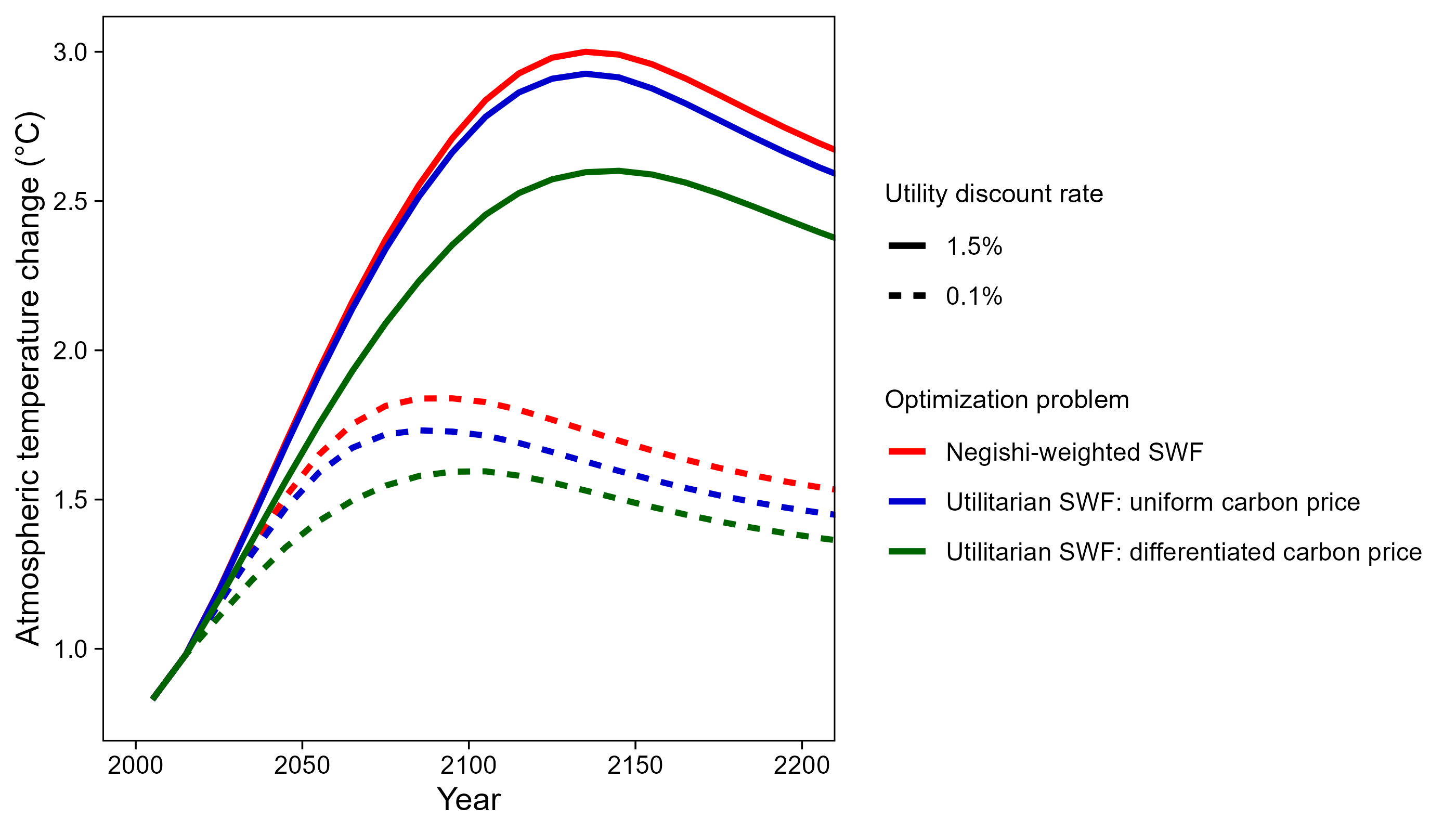
Figure 3: Optimal atmospheric temperature trajectories conditional on the optimization problem and the utility discount rate.

Notes: The Negishi-weighted solutions (red) are compared to the solutions under the utilitarian objective with (green) and without (blue) the additional constraint of equalized regional carbon prices for the Nordhaus (solid lines) and Stern (dashed lines) utility discount rates [undefaag, undefaaab]. Temperature changes are relative to 1900.

The first main result is that accounting for global inequality increases the optimal climate policy stringency in the RICE model; the utilitarian solutions with uniform and differentiated carbon prices yield lower optimal temperature trajectories than the Negishi solution. Allowing for differentiated carbon prices in the utilitarian optimization results in the lowest warming by accounting for inequality in determining both the carbon price level and differentiation. Figure 3 also shows the well-known large sensitivity of optimal climate policy to the utility discount rate. Specifically, peak warming is 3.00°C (1.84°C) in the Negishi solution, 2.93°C (1.73°C) in the utilitarian solution with uniform carbon prices, and 2.60°C (1.59°C) in the utilitarian solution with differentiated carbon prices for the 1.5% (0.1%) utility discount rate.

The corresponding cumulative global industrial carbon dioxide emissions for the entire model horizon from 2005-2595 are shown in Table A1 in the appendix. The effect of increased optimal abatement in the utilitarian solutions relative to the Negishi solution is larger for the lower utility discount rate, when the welfare impacts of future damages are given comparatively greater weight. Specifically, relative to the Negishi solution, cumulative global industrial CO₂ emissions are around 5% (13%) lower for the utilitarian solution with the additional constraint of uniform carbon prices, and 21% (27%) lower for the utilitarian differentiated carbon price solution, using the 1.5% (0.1%) utility discount rate.

The optimal carbon prices in 2025 are shown in Table 3 (the full carbon price trajectories are shown in Figure A2 in the appendix, along with the corresponding emissions). Welfare-maximizing uniform carbon prices exceed the Negishi-weighted carbon prices for both utility discount rates; specifically, by 15% (21%) under the 1.5% (0.1%) utility discount rate.

Table 3: Optimal carbon price in 2025 (in 2022 $/tCO₂) depending on the optimization problem and the utility discount rate ($\rho$).

Optimization problem	Utility discount rate
	$\rho=1.5\%$	$\rho=0.1\%$
A) Negishi-weighted SWF	25	100*
B) Utilitarian SWF: uniform carbon price	29	121
C) Utilitarian SWF: differentiated carbon price
US	338	$>410$
Other High Income	233	$>501$
Japan	232	$>638$
EU	199	$>638$
Russia	78	$>273$
Latin America	48	202
Middle East	44	182
China	32	134
Eurasia	24	103
Other Asia	10	44
India	10	41
Africa	5	23

Notes: Mimi-RICE-plus only yields an approximately equalized carbon price for the Negishi solution. In this case (*), it varied between 98 and 102 $/tCO₂ across regions. The “$>$” sign indicates that the regional backstop price has been reached. Thus, any price above the backstop price is optimal as complete abatement is required.

Furthermore, to reduce the welfare cost of abatement, there are large differences in welfare-maximizing carbon prices between regions when the constraint of equalized carbon prices is not imposed. Consistent with the theoretical results in Section 3.2, this yields high carbon prices in rich regions – exceeding $\sim$$200/tCO₂, even for the high utility discount rate – and much lower carbon prices in poor regions. For the lower Stern utility discount rate, the richest five regions already reach their backstop price in 2025, resulting in zero carbon emissions. Notably, the utilitarian differentiated carbon prices exceed the Negishi-weighted carbon prices for all regions but the poorest three (or four) regions. This also results in large regional changes in cumulative emissions compared to the Negishi solution, featuring substantial emission reductions in rich regions, smaller reductions in middle-income regions, and emission increases in the poorest three regions (see Figure A3 in the appendix). Importantly, the emission reductions in rich and middle-income regions outweigh the emission increases in the poorest regions, resulting in lower global emissions compared to the Negishi solution. The differentiated carbon price optimum is discussed in more detail in Appendix C.4.

4.2.2 Regional heterogeneities and distributional effects

Why do the utilitarian maximizations lead to greater climate policy ambition compared to the Negishi solution? This section addresses this question by analyzing the distributional impacts of the different climate policy pathways and the regional heterogeneities that drive these outcomes.

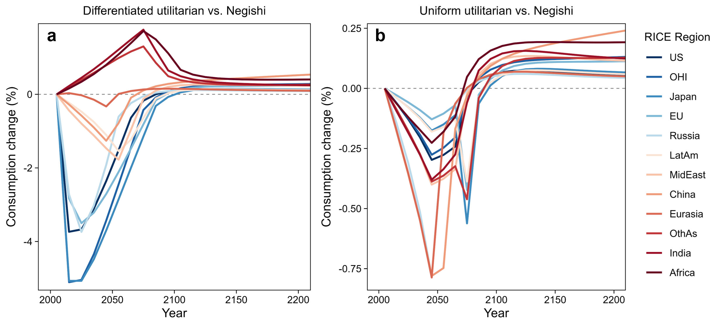
Figure A6: Relative regional consumption changes between the Negishi solution and the utilitarian solutions.

I begin by examining which regions are better off and which are worse off under the utilitarian solutions compared to the Negishi solution. To provide a simple summary statistic that shows which regions gain or lose overall over the entire model horizon, I focus on regions’ aggregate intertemporal welfare changes, expressed as the net present value (NPV) of consumption changes over time. These regional NPV consumption changes are shown in Figure 4 along with the global welfare gains of the utilitarian solutions (the temporal trajectories in consumption changes are shown in Figure A6 in the appendix). More specifically, I compute the consumption changes in the initial period (2005) that would yield a welfare change (in utility terms) that is equivalent to the welfare difference between each of the utilitarian solutions and the Negishi solution. Global utilitarian welfare changes are expressed in the welfare-equivalent consumption change in 2005 if consumption were distributed equally. Details of this calculation are provided in Appendix A.10. For the remainder of the numerical results, I focus on the 1.5% utility discount rate to streamline the discussion. Additional results for the 0.1% utility discount rate are shown in the appendix.

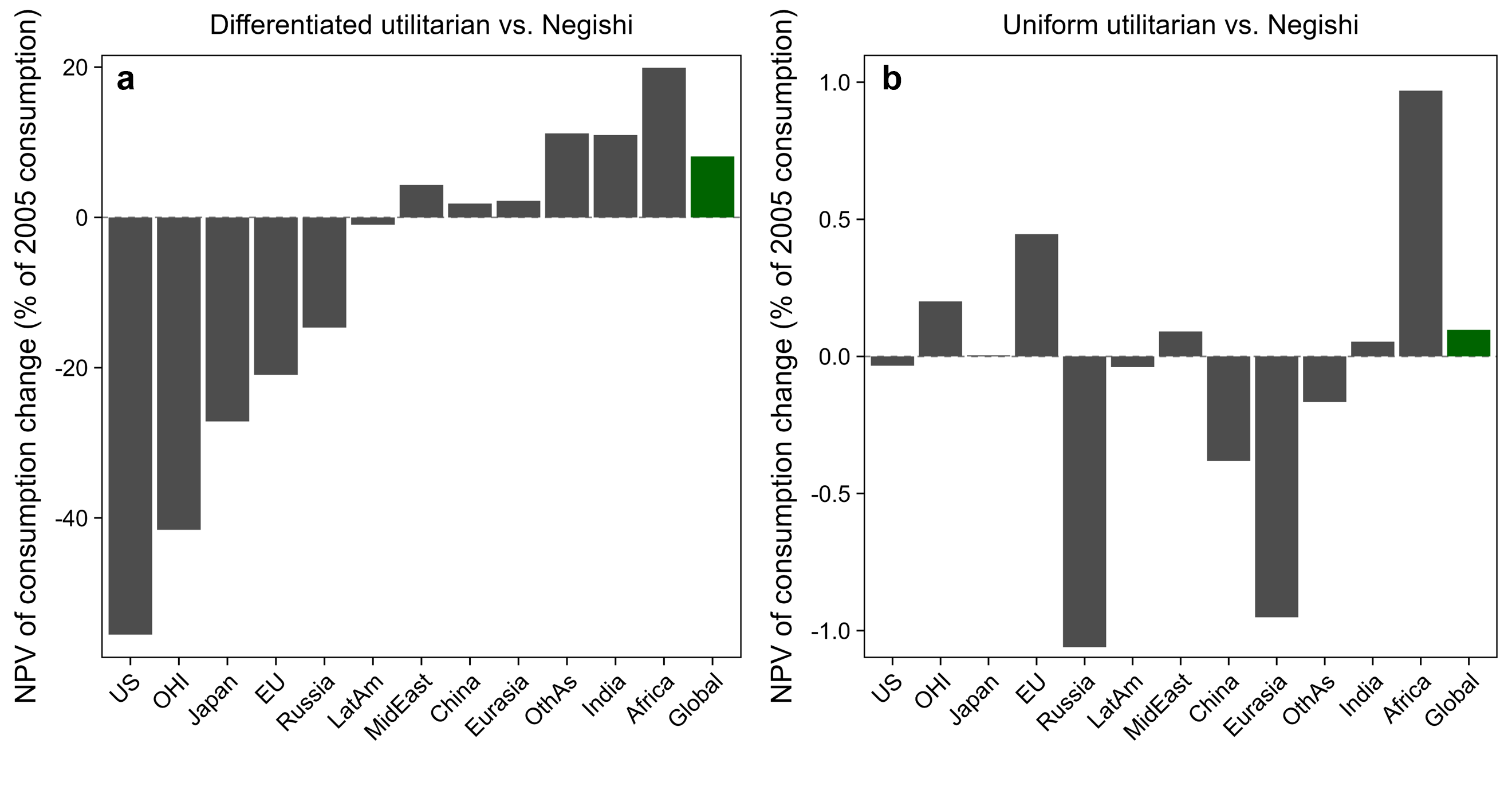
Figure 4: Net present value of consumption changes.

Notes: The values show the welfare-equivalent consumption change in 2005, as a percentage of the consumption in 2005. The “Global” value expresses the global utilitarian welfare change in the welfare-equivalent consumption change in 2005 if consumption were distributed equally (for details, see Appendix A.10). The figure shows the results for the utility discount rate of 1.5%.

The comparison of the utilitarian differentiated carbon price solution and the Negishi solution is straightforward: rich regions are better off in the Negishi solution and poor regions are better off in the utilitarian solution (see Figure 4a). Most importantly, global (unweighted) welfare is higher in the utilitarian solution. This is of course unsurprising since the utilitarian SWF measures global (unweighted) welfare and Negishi weights upweight the welfare of rich regions and downweight the welfare of poor regions. The poorest four regions are better off in all periods in the utilitarian solution, due to both lower abatement costs in their regions and lower global emissions. In contrast, rich regions experience NPV consumption losses as a result of higher abatement costs associated with increased carbon prices. Crucially, however, all regions enjoy consumption gains after 2150 because of reduced climate damages due to reduced global emissions (see Figure A6a). Thus, the increased abatement in rich regions does not lead to persistently lower consumption trajectories. In addition, it is worth noting that the consumption losses in rich regions do not imply negative consumption per capita growth rates. More generally, the consumption per capita trajectories of all regions are not affected substantially, especially compared to the magnitude of the inequality across regions. Thus, while the utilitarian solutions result in greater global welfare by accounting for global inequality in setting the carbon prices, they do not solve the inequality issue.

The distributional consequences are more complicated for the uniform carbon price solutions. The region that benefits the most from higher carbon prices in the utilitarian solution relative to the Negishi solution is the poorest region, Africa (see Figure 4b). Indeed, the intertemporal welfare gain in utility terms is by far the largest in Africa (see Figure A9b in the appendix). This indicates that the lower carbon prices in the Negishi solution are primarily driven by the down-weighting of Africa in the Negishi-weighted SWF. I have confirmed this through a model run in which Africa is removed from the utilitarian social welfare function. Further analysis reveals that the difference in optimal policy stringency between the utilitarian and Negishi solutions is driven by disproportionately large climate damages in Africa. While all regions benefit again in the long-term, Russia and Eurasia experience the greatest consumption losses in NPV terms due to increased abatement costs.

To understand the underlying drivers of the distributional effects for the uniform carbon price solutions we can leverage the results from the theory model. Proposition 4 and Equation (20) show that relatively higher marginal damages and a more convex abatement cost function in the South, compared to the North, contribute to a higher uniform carbon price in the utilitarian solution than in the Negishi solution. Figure 5 examines whether this is the case in the RICE model, showing the ratios of the regional marginal damages and convexities of the abatement cost functions (both as a percentage of GDP in 2025) relative to the US. Marginal damages are estimated as the present value (in 2025) of the stream of damages associated with a marginal pulse of emissions in 2025 (using region-specific discount rates).

Figure 5: Relative regional marginal damages and abatement cost convexities.

Notes: The ratio of the 2025 present values (PV) of the stream of regional marginal damages as a percentage of the regional GDP in 2025, $\mathbf{d}^{\prime}_{i}$, is given by $PV(\mathbf{d}^{\prime}_{i})/PV(\mathbf{d}^{\prime}_{US})$. The ratio of the convexities in the abatement cost functions is $c^{\prime\prime}_{i,t}/c^{\prime\prime}_{US,t}$ (evaluated at uniform carbon prices), where $t$ is the year 2025. Panel (b) shows regions’ Negishi and utilitarian welfare weights in 2025 relative to the weights in the US. The figure shows the results for the utility discount rate of 1.5%.

Consistent with the theoretical results, Figure 5 shows that the regions that enjoy NPV consumption gains from the higher utilitarian carbon prices tend to have relatively high marginal damages and/or more convex abatement cost functions. Most notably, Africa is the region with the largest marginal damages relative to the size of its economy. Additionally, Africa has a fairly convex abatement cost function, which reduces its abatement cost burden as carbon prices are increased. Together, these two attributes explain why Africa experiences the largest gains in NPV consumption. The strongly convex abatement cost function in the EU is also noteworthy, resulting in NPV gains in the EU from the higher utilitarian carbon prices. Conversely, Russia and Eurasia experience the largest NPV losses due to relatively low marginal damages and flatter marginal abatement cost curves.

As the poorest region, Africa receives the lowest Negishi weight, which is roughly 70 times smaller than that of the richest region, the US, in 2025 (see Figure 5b). Intuitively, the heavy down-weighting of welfare in the region most impacted by climate damages is a key factor behind the lower carbon prices in the Negishi solution.

Figure A12 in the appendix provides a more detailed breakdown of the regional heterogeneities that give rise to differential climate impacts. Rather than computing the present values of the stream of marginal damages, which are affected by population growth and economic growth, it shows the undiscounted marginal damages as a percentage of GDP in a given year alongside population and economic growth. Building on the theoretical insights from the dynamic model, this figure shows that Africa is particularly strongly affected by climate change, not only due to its high climate damages as a percentage of GDP but also because it has the fastest population growth, amplifying the aggregate damages by increasing the number of people affected. However, counterbalancing this to some degree is Africa’s fast economic growth, which causes Africa’s climate damages to be more heavily discounted under the utilitarian SWF.

4.2.3 Regions’ preferred uniform carbon prices

This section presents the preferred uniform carbon prices for different regions, offering a complementary perspective on why utilitarian welfare weights lead to higher uniform carbon prices than Negishi weights. Drawing on the theoretical two-region model from Section 3.4, we know that this occurs if and only if the poorer region prefers a higher uniform carbon price than the richer region. By examining these preferences within the RICE model, we can gain further intuition for this result. Additionally, understanding regions’ preferences regarding uniform carbon prices is valuable in its own right, as it helps to identify which regions might advocate for more or less stringent global climate policies in international negotiations.

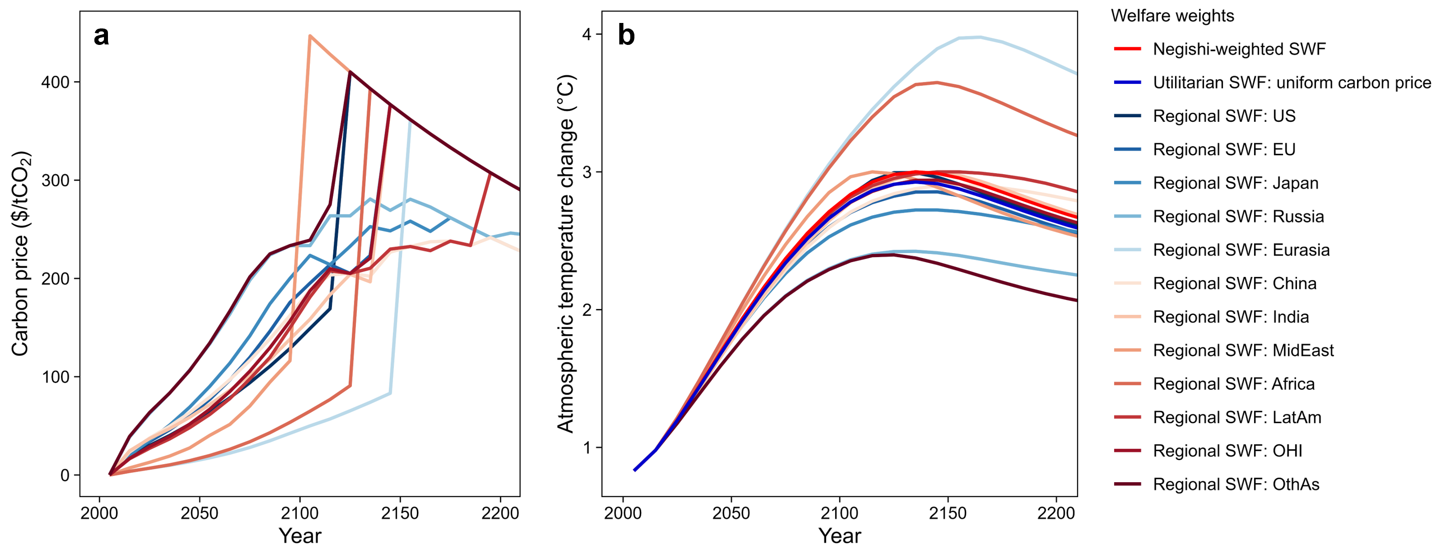
Figure A13: Regions’ preferred uniform carbon prices and corresponding temperature trajectories.

Table 4 shows each region’s preferred uniform carbon prices and the resulting peak temperature increase (the full carbon price and temperature trajectories are shown in Figure A13 in the appendix). The preferred uniform carbon prices vary widely across regions. In 2025, they differ by nearly an order of magnitude, from $7 per ton of CO₂ in Russia and Eurasia to over $60 per ton in Africa and the EU. This also leads to significant differences in peak temperatures, with Africa’s preferred policy limiting warming to 2.4°C, while Russia’s preferred policy allows for nearly 4°C.

Table 4: Regions preferred uniform carbon prices (in 2022 $/tCO₂) and resulting peak warming. For comparison, the uniform utilitarian and Negishi-weighted carbon prices are also shown.

	Carbon prices
Welfare weights	2025	2055	2085	Peak warming (°C)
Negishi	25	60*	116**	3.00
Utilitarian	29	68	128	2.93
US	30	64	111	2.99
OHI	34	77	146	2.86
Japan	35	90	174	2.72
EU	63	133	224	2.42
Russia	7	17	35	3.98
LatAm	38	79	138	2.91
MidEast	37	72	118	3.00
China	13	40	94	3.00
Eurasia	7	20	43	3.65
OthAs	27	62	120	3.00
India	29	67	129	2.94
Africa	64	134	225	2.40

Notes: The table shows the results for the utility discount rate of 1.5%. Temperature changes are relative to 1900. Mimi-RICE-plus only yields an approximately equalized carbon price for the Negishi solution. Specifically, it varied across regions between (*) 59 and 63 $/tCO₂ in 2055, and (**) 113 and 121 $/tCO₂ in 2085.

The large differences in regions’ preferred uniform carbon prices highlight the importance of how these preferences are weighted in the SWF. This perspective provides additional intuition for why optimal carbon prices are lower in the Negishi solution, which downweights the preferences of poorer regions. Notably, Africa, the poorest region that is most heavily downweighted in the Negishi-weighted SWF, has the highest preferred carbon prices, mainly due to its disproportionately large climate damages. In contrast, the US, the region with the largest Negishi weights, prefers comparatively low carbon prices, particularly after 2050. Specifically, Africa’s preferred uniform carbon prices are more than twice as high as those of the US. While the overall effect depends on all regions, the downweighting of Africa’s preferences is the primary reason for lower carbon prices in the Negishi solution compared to the utilitarian solution, which assigns equal weight to all regions’ welfare, as discussed above.

5 Conclusion

This paper investigates how accounting for inequality affects optimal carbon prices. Specifically, it compares the optimal carbon prices under two optimization approaches: the conventional, positive approach which maximizes the Negishi-weighted social welfare function (SWF), and a normative approach which focuses on maximizing global welfare, employing constrained maximizations of the utilitarian SWF.

Using a theoretical model, I show that, in the absence of international transfers, accounting for inequality may result in higher or lower optimal carbon prices and that this depends on regional differences in marginal climate damages and the burden of abatement costs, and disparities in population and economic growth. Intuitively, global welfare maximization warrants more stringent climate policy if poor countries are more vulnerable to future climate change—due to higher marginal damages, faster population growth and slow economic catch-up—and if the cost burden of abatement predominately falls on rich countries. This highlights the importance of accurately accounting for regional heterogeneities in climate economic model. In numerical simulations with the integrated assessment model RICE, I find that accounting for inequality results in lower optimal global emissions, both if carbon prices are allowed to be regionally differentiated and if they are constrained to be globally uniform.

There are some limitations of this study which are left for future research. First, the RICE model masks inequality within its twelve regions. Thus, a valuable avenue for future research would be to account for inequality at a finer resolution and examine how the quantitative results change. Existing modifications of the RICE model may be used for this analysis, such as NICE and RICE50+ [undefad, undefan].

Second, the numerical simulations of this study are performed with a single integrated assessment model (IAM). As different IAMs are known to produce different results, it would be worthwhile to replicate the analysis with other IAMs to assess the robustness of the findings of this paper. Furthermore, it would be valuable to strengthen the empirical evidence on regional heterogeneities highlighted by this paper’s theoretical results, including differences in damage and abatement cost functions, as well as in economic and population growth.

Third, this study relies on deterministic models. Given the substantial uncertainties in both human and physical systems and the associated economic effects of climate change, extending the analysis to a probabilistic framework would be valuable. Building on the findings of this paper, it could be particularly insightful to explore potential disparities in the uncertainties that different regions face.

Appendix A: Proofs and Derivations

A.1 Derivation of optimal carbon prices

This section shows the derivation of the optimal uniform carbon price for arbitrary welfare weights (Equation A18). As discussed briefly below, the derivation of the optimal differentiated carbon prices is largely analogous (and, in fact, simpler) and therefore not explicitly shown.

The Lagrangian of the uniform carbon price optimization problem is

$$\begin{aligned} \mathcal{L}=L_{i}\alpha_{i}u\left(\frac{X_{i}}{L_{i}}\right)&-\sum_{i}\lambda_{i}\left(X_{i}-W_{i}+C_{i}(A_{i})+D_{i}(A)\right)\\ &-\mu\left(C^{\prime}_{N}(A_{N})-C^{\prime}_{S}(A_{S})\right),\end{aligned}$$

where $\lambda_{i}$ and $\mu$ are Lagrange multipliers.

The first-order conditions (FOCs) are:

$$\begin{aligned} &[X_{i}]:\alpha_{i}u^{\prime}(x_{i})=\lambda_{i},\quad\forall i\\ &[A_{N}]:\lambda_{N}C^{\prime}_{N}(A_{N})=-\sum_{i}\lambda_{i}D_{i}^{\prime}(A)-\mu C^{\prime\prime}_{N}\\ &[A_{S}]:\lambda_{S}C^{\prime}_{S}(A_{S})=-\sum_{i}\lambda_{i}D_{i}^{\prime}(A)+\mu C^{\prime\prime}_{S}\\ &[\lambda_{i}]:X_{i}=W_{i}-C_{i}(A_{i})-D_{i}(A),\quad\forall i\\ &[\mu]:C^{\prime}_{N}(A_{N})=C^{\prime}_{S}(A_{S}).\end{aligned}$$

Combining the FOCs, we get the following two optimality conditions:

$$\alpha_{N}u^{\prime}(x_{N})C^{\prime}_{N}(A_{N})=-\sum_{i}\alpha_{i}u^{\prime}(x_{i})D_{i}^{\prime}(A)-\mu C^{\prime\prime}_{N},$$ (A1)

$$\alpha_{S}u^{\prime}(x_{S})C^{\prime}_{S}(A_{S})=-\sum_{i}\alpha_{i}u^{\prime}(x_{i})D_{i}^{\prime}(A)+\mu C^{\prime\prime}_{S}.$$ (A2)

We can now solve these two equations for the optimal uniform carbon price, noting that $C^{\prime}_{N}(A_{N})=C^{\prime}_{S}(A_{S})$ by the uniform carbon price constraint. Eliminating $\mu$ by dividing Equation (A1) by Equation (A2), and simple manipulations yield the optimal uniform carbon price (Equation (A18) in the main text),

$$\tau^{uni}=C^{\prime}_{i}(A_{i}^{*})=-\sum_{i}\alpha_{i}u^{\prime}(x_{i}^{*})D^{\prime}_{i}(A^{*})\frac{C^{\prime\prime}_{S}+C^{\prime\prime}_{N}}{\alpha_{N}u^{\prime}(x_{N}^{*})C^{\prime\prime}_{S}+\alpha_{S}u^{\prime}(x_{S}^{*})C^{\prime\prime}_{N}}.$$

The derivation of the optimal differentiated carbon price is largely analogous. The main difference is that the uniform carbon price constraint is missing (i.e., $\mu(C^{\prime}_{N}(A_{N})-C^{\prime}_{S}(A_{S}))$ is missing in the Lagrangian). Hence, we (generally) get different optimal carbon prices in the two regions.

A.2 Derivation of optimality conditions

A.2.1 Negishi solution

We start with Equation (6),

$$\frac{d{C}_{i}(\tilde{A}_{i})}{d\tilde{A}_{i}}=-\sum_{i}\frac{d{D}_{i}(\tilde{A})}{d\tilde{A}}.$$

Multiplying both sides by $\frac{d\tilde{A}}{d\tilde{\tau}}$, and using $d\tilde{A}=d\tilde{A}_{S}+d\tilde{A}_{N}$, yields

$$\frac{d{C}_{i}(\tilde{A}_{i})}{d\tilde{A}_{i}}\frac{d\tilde{A}_{S}+d\tilde{A}_{N}}{d\tilde{\tau}}=-\sum_{i}\frac{d{D}_{i}(\tilde{A})}{d\tilde{\tau}}.$$

Using $\tilde{\tau}=\frac{d{C}_{N}(\tilde{A}_{N})}{d\tilde{A}_{N}}=\frac{d{C}_{S}(\tilde{A}_{S})}{d\tilde{A}_{S}}$, we obtain

$$\sum_{i}\frac{d{C}_{i}(\tilde{A}_{i})}{d\tilde{\tau}}=-\sum_{i}\frac{d{D}_{i}(\tilde{A})}{d\tilde{\tau}}.$$

A.2.2 Utilitarian uniform carbon price solution

We start with Equation (8),

$$\frac{d{C}_{i}(\check{A}_{i})}{d\check{A}_{i}}=-\sum_{i}{u}^{\prime}(\check{x}_{i})\frac{d{D}_{i}(\check{A})}{d\check{A}}\frac{{C}^{\prime\prime}_{S}+{C}^{\prime\prime}_{N}}{{u}^{\prime}(\check{x}_{N}){C}^{\prime\prime}_{S}+{u}^{\prime}(\check{x}_{S}){C}^{\prime\prime}_{N}}.$$

Using $C^{\prime\prime}_{i}=\frac{d\check{C}^{\prime}_{i}}{d\check{A}_{i}}=\frac{d\check{\tau}}{d\check{A}_{i}}$, multiplying both sides by $\frac{d\check{A}}{d\check{\tau}}$ and rearranging, we have

$$\frac{d{C}_{i}(\check{A}_{i})}{d\check{A}_{i}}\frac{{u}^{\prime}(\check{x}_{N})\frac{d\check{A}}{d\check{A}_{S}}+{u}^{\prime}(\check{x}_{S})\frac{d\check{A}}{d\check{A}_{N}}}{\frac{d\check{\tau}}{d\check{A}_{S}}+\frac{d\check{\tau}}{d\check{A}_{N}}}=-\sum_{i}{u}^{\prime}(\check{x}_{i})\frac{d{D}_{i}(\check{A})}{d\check{\tau}}.$$

Using $\frac{d{C}_{S}(\check{A}_{S})}{d\check{A}_{S}}=\frac{d{C}_{N}(\check{A}_{N})}{d\check{A}_{N}}$, equalizing the denominators of the ratios in the denominator and rearranging yields

$$\begin{gathered}{u}^{\prime}(\check{x}_{N})\frac{d\check{A}}{d\check{A}_{S}d\check{\tau}}\frac{dC_{S}(\check{A}_{S})dC_{N}(\check{A}_{N})}{dC_{S}(\check{A}_{S})+dC_{N}(\check{A}_{N})}+{u}^{\prime}(\check{x}_{S})\frac{d\check{A}}{d\check{A}_{N}d\check{\tau}}\frac{dC_{S}(\check{A}_{S})dC_{N}(\check{A}_{N})}{dC_{S}(\check{A}_{S})+dC_{N}(\check{A}_{N})}\\ =-\sum_{i}{u}^{\prime}(\check{x}_{i})\frac{d{D}_{i}(\check{A})}{d\check{\tau}}.\end{gathered}$$

Using $\check{\tau}=\frac{d\check{C}_{S}}{d\check{A}_{S}}=\frac{d\check{C}_{N}}{d\check{A}_{N}}$, and thus $\check{\tau}d\check{A}_{i}=d\check{C}_{i}$ for all $i$, we rewrite the previous equation as

$$\check{\tau}\frac{d\check{A}_{S}+d\check{A}_{N}}{\check{\tau}d\check{A}_{S}+\check{\tau}d\check{A}_{N}}\left({u}^{\prime}(\check{x}_{N})\frac{dC_{N}(\check{A}_{N})}{d\check{\tau}}+{u}^{\prime}(\check{x}_{S})\frac{dC_{S}(\check{A}_{S})}{d\check{\tau}}\right)=-\sum_{i}{u}^{\prime}(\check{x}_{i})\frac{d{D}_{i}(\check{A})}{d\check{\tau}},$$

which simplifies to

$$\sum_{i}{u}^{\prime}(\check{x}_{i})\frac{dC_{i}(\check{A}_{i})}{d\check{\tau}}=-\sum_{i}{u}^{\prime}(\check{x}_{i})\frac{d{D}_{i}(\check{A})}{d\check{\tau}}.$$

A.2.3 Regions’ preferred uniform carbon price

We start with Equation (13),

$$\frac{d{C}_{i}(\mathring{A}_{i}^{i})}{d\mathring{A}_{i}^{i}}=-\frac{d{D}_{i}(\mathring{A^{i}})}{d\mathring{A^{i}}}\frac{{C}^{\prime\prime}_{i}+{C}^{\prime\prime}_{-i}}{{C}^{\prime\prime}_{-i}},$$

Using ${C}^{\prime\prime}_{i}=\frac{d{C}^{\prime}_{i}(\mathring{A}_{i}^{i})}{d\mathring{A}_{i}^{i}}=\frac{d\mathring{\tau}^{i}}{d\mathring{A}_{i}^{i}}$ and ${C}^{\prime\prime}_{i}=\frac{d{C}^{\prime}_{-i}(\mathring{A}_{-i}^{i})}{d\mathring{A}_{-i}^{i}}=\frac{d\mathring{\tau}^{i}}{d\mathring{A}_{-i}^{i}}$, multiplying both sides by $\frac{d\check{A}}{d\check{\tau}}$ and rearranging, we have

$$\begin{aligned} \frac{d{C}_{i}(\mathring{A}_{i}^{i})}{d\mathring{A}_{i}^{i}}&=-\frac{d{D}_{i}(\mathring{A^{i}})}{d\mathring{A^{i}}}\frac{\frac{d\mathring{\tau}^{i}}{d\mathring{A}_{i}^{i}}+\frac{d\mathring{\tau}^{i}}{d\mathring{A}_{-i}^{i}}}{\frac{d\mathring{\tau}^{i}}{d\mathring{A}_{-i}^{i}}}\\ &=-\frac{d{D}_{i}(\mathring{A^{i}})}{d\mathring{A^{i}}}\left(\frac{d\mathring{A}_{-i}^{i}}{d\mathring{A}_{i}^{i}}+1\right)\\ &=-\frac{d{D}_{i}(\mathring{A^{i}})}{d\mathring{A^{i}}}\left(\frac{d\mathring{A}_{-i}^{i}+d\mathring{A}_{i}^{i}}{d\mathring{A}_{i}^{i}}\right)\\ &=-\frac{d{D}_{i}(\mathring{A^{i}})}{d\mathring{A^{i}_{i}}}.\end{aligned}$$

Multiplying both sides by $\frac{d\mathring{A}^{i}_{i}}{d\mathring{\tau}^{i}}$, we obtain

$$\frac{d{C}_{i}(\mathring{A}_{i}^{i})}{d\mathring{\tau}^{i}}=-\frac{d{D}_{i}(\mathring{A^{i}})}{d\mathring{\tau}^{i}}.$$

A.3 Proof of Proposition 1

Proof.

We split the proof into the forward and backward implications.

Proof of forward implicationProof of forward implicationProof of forward implicationProof of forward implicationProof of forward implicationProof of forward implicationProof of forward implicationProof of forward implicationProof of forward implicationProof of forward implicationProof of forward implicationProof of forward implicationProof of forward implicationProof of forward implicationProof of forward implicationProof of forward implicationProof of forward implicationProof of forward implication: $\tilde{\tau}<\check{\tau}$ $\implies$ $\frac{\check{D}^{\prime}_{S}}{\check{D}^{\prime}_{N}}>\frac{C^{\prime\prime}_{N}}{C^{\prime\prime}_{S}}$.

Let us ask under which conditions $\tilde{\tau}<\check{\tau}$, or equivalently, $\tilde{C}^{\prime}<\check{C}^{\prime}$. First note that, for strictly convex abatement cost functions, $\tilde{C}^{\prime}<\check{C}^{\prime}$ implies $\tilde{A}_{i}<\check{A}_{i}$ for all $i$, and thus $\tilde{A}<\check{A}$. For strictly convex damage functions, this implies $\tilde{D}^{\prime}_{i}<\check{D}^{\prime}_{i}$ for all $i$ (note that marginal damages of abatement are negative).

We have $\tilde{C}^{\prime}<\check{C}^{\prime}$ if and only if

$$-\tilde{D}^{\prime}_{N}-\tilde{D}^{\prime}_{S}<(-\check{u}^{\prime}_{N}\check{D}^{\prime}_{N}-\check{u}^{\prime}_{S}\check{D}^{\prime}_{S})\frac{C^{\prime\prime}_{S}+C^{\prime\prime}_{N}}{\check{u}^{\prime}_{N}C^{\prime\prime}_{S}+\check{u}^{\prime}_{S}C^{\prime\prime}_{N}}.$$

Multiplying both sides by the denominator on the right-hand side (which is positive), and rearranging, we get

$$(\check{u}^{\prime}_{N}\check{D}^{\prime}_{N}+\check{u}^{\prime}_{S}\check{D}^{\prime}_{S})(C^{\prime\prime}_{S}+C^{\prime\prime}_{N})<(\tilde{D}^{\prime}_{N}+\tilde{D}^{\prime}_{S})(\check{u}^{\prime}_{N}C^{\prime\prime}_{S}+\check{u}^{\prime}_{S}C^{\prime\prime}_{N}).$$

Multiplying out and collecting terms, we have

$$C^{\prime\prime}_{N}\Bigl(\check{u}^{\prime}_{N}\check{D}^{\prime}_{N}+\check{u}^{\prime}_{S}\check{D}^{\prime}_{S}-\check{u}^{\prime}_{S}\tilde{D}^{\prime}_{N}-\check{u}^{\prime}_{S}\tilde{D}^{\prime}_{S}\Bigr)<C^{\prime\prime}_{S}\Bigl(\check{u}^{\prime}_{N}\tilde{D}^{\prime}_{N}+\check{u}^{\prime}_{N}\tilde{D}^{\prime}_{S}-\check{u}^{\prime}_{N}\check{D}^{\prime}_{N}-\check{u}^{\prime}_{S}\check{D}^{\prime}_{S}\Bigr).$$ (A3)

We know that $\Bigl(\check{u}^{\prime}_{N}\check{D}^{\prime}_{N}+\check{u}^{\prime}_{S}\check{D}^{\prime}_{S}-\check{u}^{\prime}_{S}\tilde{D}^{\prime}_{N}-\check{u}^{\prime}_{S}\tilde{D}^{\prime}_{S}\Bigr)>0$ if $\check{u}^{\prime}_{S}>\check{u}^{\prime}_{N}$ and $\tilde{D}^{\prime}_{i}<\check{D}^{\prime}_{i}$ because $\check{u}^{\prime}_{S}\check{D}^{\prime}_{S}-\check{u}^{\prime}_{S}\tilde{D}^{\prime}_{S}>0$ since $\tilde{D}^{\prime}_{i}<\check{D}^{\prime}_{i}$ and $\check{u}^{\prime}_{N}\check{D}^{\prime}_{N}-\check{u}^{\prime}_{S}\tilde{D}^{\prime}_{N}>0$ since $\check{u}^{\prime}_{S}>\check{u}^{\prime}_{N}$ and $\tilde{D}^{\prime}_{i}<\check{D}^{\prime}_{i}$. Hence, we can divide by it and the sign of the inequality does not flip. Moreover, note that we must also have

$$\Bigl(\check{u}^{\prime}_{N}\tilde{D}^{\prime}_{N}+\check{u}^{\prime}_{N}\tilde{D}^{\prime}_{S}-\check{u}^{\prime}_{N}\check{D}^{\prime}_{N}-\check{u}^{\prime}_{S}\check{D}^{\prime}_{S}\Bigr)>0$$ (A4)

for the inequality in Equation (A3) to hold, since $C_{i}^{\prime\prime}>0$ for all $i$.

Cross-division, collecting common terms, and rearranging yields

$$\frac{C^{\prime\prime}_{N}}{C^{\prime\prime}_{S}}<\frac{\check{u}^{\prime}_{N}(\tilde{D}^{\prime}_{N}-\check{D}^{\prime}_{N}+\tilde{D}^{\prime}_{S})-\check{u}^{\prime}_{S}\check{D}^{\prime}_{S}}{\check{u}^{\prime}_{N}\check{D}^{\prime}_{N}-\check{u}^{\prime}_{S}(\tilde{D}^{\prime}_{S}-\check{D}^{\prime}_{S}+\tilde{D}^{\prime}_{N})}.$$

Note that

$$\underbrace{\tilde{D}^{\prime}_{N}-\check{D}^{\prime}_{N}}_{<0}+\tilde{D}^{\prime}_{S}<\tilde{D}^{\prime}_{S}$$

and

$$\underbrace{\tilde{D}^{\prime}_{S}-\check{D}^{\prime}_{S}}_{<0}+\tilde{D}^{\prime}_{N}<\tilde{D}^{\prime}_{N}$$

Thus, for the numerator we have

$$\begin{aligned} \overbrace{\check{u}^{\prime}_{N}\underbrace{(\tilde{D}^{\prime}_{N}-\check{D}^{\prime}_{N}+\tilde{D}^{\prime}_{S})}_{<\tilde{D}^{\prime}_{S}}-\check{u}^{\prime}_{S}\check{D}^{\prime}_{S}}^{>0\text{ by Equation~\eqref{E: UvN positivity condition} }}&<\check{u}^{\prime}_{N}\tilde{D}^{\prime}_{S}-\check{u}^{\prime}_{S}\check{D}^{\prime}_{S}\\ &<\check{u}^{\prime}_{N}\check{D}^{\prime}_{S}-\check{u}^{\prime}_{S}\check{D}^{\prime}_{S}\\ &>0,\end{aligned}$$

where the second inequality holds since $\tilde{D}^{\prime}_{S}<\check{D}^{\prime}_{S}$ and the last inequality holds since $\check{u}^{\prime}_{S}>\check{u}^{\prime}_{N}$.

Similarly, for the denominator, we have

$$\begin{aligned} \check{u}^{\prime}_{N}\check{D}^{\prime}_{N}-\check{u}^{\prime}_{S}\underbrace{(\tilde{D}^{\prime}_{S}-\check{D}^{\prime}_{S}+\tilde{D}^{\prime}_{N})}_{<\tilde{D}^{\prime}_{N}}&>\check{u}^{\prime}_{N}\check{D}^{\prime}_{N}-\check{u}^{\prime}_{S}\tilde{D}^{\prime}_{N}\\ &>\check{u}^{\prime}_{N}\check{D}^{\prime}_{N}-\check{u}^{\prime}_{S}\check{D}^{\prime}_{N}\\ &>0,\end{aligned}$$

where the second inequality holds since $\tilde{D}^{\prime}_{S}<\check{D}^{\prime}_{S}$ and the last inequality holds since $\check{u}^{\prime}_{S}>\check{u}^{\prime}_{N}$.

Compared to the case “Negishi = Utilitarian”, we have a greater (positive) denominator, and a smaller (positive, by Equation (A4)) numerator.

Putting this together we have

$$\begin{aligned} \frac{C^{\prime\prime}_{N}}{C^{\prime\prime}_{S}}&<\frac{\check{u}^{\prime}_{N}(\tilde{D}^{\prime}_{N}-\check{D}^{\prime}_{N}+\tilde{D}^{\prime}_{S})-\check{u}^{\prime}_{S}\check{D}^{\prime}_{S}}{\check{u}^{\prime}_{N}\check{D}^{\prime}_{N}-\check{u}^{\prime}_{S}(\tilde{D}^{\prime}_{S}-\check{D}^{\prime}_{S}+\tilde{D}^{\prime}_{N})}\\ &<\frac{\check{u}^{\prime}_{N}\check{D}^{\prime}_{S}-\check{u}^{\prime}_{S}\check{D}^{\prime}_{S}}{\check{u}^{\prime}_{N}\check{D}^{\prime}_{N}-\check{u}^{\prime}_{S}\check{D}^{\prime}_{N}}\\ &=\frac{\check{D}^{\prime}_{S}}{\check{D}^{\prime}_{N}}.\end{aligned}$$

We have thus shown that $\tilde{C}^{\prime}<\check{C}^{\prime}\implies\frac{\check{D}^{\prime}_{S}}{\check{D}^{\prime}_{N}}>\frac{C^{\prime\prime}_{N}}{C^{\prime\prime}_{S}}$.

Proof of backward implicationProof of backward implicationProof of backward implicationProof of backward implicationProof of backward implicationProof of backward implicationProof of backward implicationProof of backward implicationProof of backward implicationProof of backward implicationProof of backward implicationProof of backward implicationProof of backward implicationProof of backward implicationProof of backward implicationProof of backward implicationProof of backward implicationProof of backward implication: $\frac{\check{D}^{\prime}_{S}}{\check{D}^{\prime}_{N}}>\frac{C^{\prime\prime}_{N}}{C^{\prime\prime}_{S}}$ $\implies$ $\tilde{\tau}<\check{\tau}$.

In order to derive a contradiction, suppose that $\frac{\check{D}^{\prime}_{S}}{\check{D}^{\prime}_{N}}>\frac{C^{\prime\prime}_{N}}{C^{\prime\prime}_{S}}$ $\implies$ $\tilde{\tau}\geq\check{\tau}$.

We begin by establishing the implications of $\tilde{\tau}\geq\check{\tau}$, or equivalently, $\tilde{C}^{\prime}\geq\check{C}^{\prime}$. First note that, for strictly convex abatement cost functions, $\tilde{C}^{\prime}\geq\check{C}^{\prime}$ implies $\tilde{A}_{i}\geq\check{A}_{i}$ for all $i$, and thus $\tilde{A}\geq\check{A}$. For strictly convex damage functions, this implies $\tilde{D}^{\prime}_{i}\geq\check{D}^{\prime}_{i}$ for all $i$ (note that marginal damages of abatement are negative).

Next, note that $\tilde{C}^{\prime}\geq\check{C}^{\prime}$ if and only if

$$-\tilde{D}^{\prime}_{N}-\tilde{D}^{\prime}_{S}\geq(-\check{u}^{\prime}_{N}\check{D}^{\prime}_{N}-\check{u}^{\prime}_{S}\check{D}^{\prime}_{S})\frac{C^{\prime\prime}_{S}+C^{\prime\prime}_{N}}{\check{u}^{\prime}_{N}C^{\prime\prime}_{S}+\check{u}^{\prime}_{S}C^{\prime\prime}_{N}}.$$

Multiplying both sides by the denominator on the right-hand side (which is positive), and rearranging, we get

$$(\check{u}^{\prime}_{N}\check{D}^{\prime}_{N}+\check{u}^{\prime}_{S}\check{D}^{\prime}_{S})(C^{\prime\prime}_{S}+C^{\prime\prime}_{N})\geq(\tilde{D}^{\prime}_{N}+\tilde{D}^{\prime}_{S})(\check{u}^{\prime}_{N}C^{\prime\prime}_{S}+\check{u}^{\prime}_{S}C^{\prime\prime}_{N}).$$

Multiplying this out and collecting common terms gives

$$C^{\prime\prime}_{N}\Bigl(\check{u}^{\prime}_{N}\check{D}^{\prime}_{N}+\check{u}^{\prime}_{S}\check{D}^{\prime}_{S}-\check{u}^{\prime}_{S}\tilde{D}^{\prime}_{N}-\check{u}^{\prime}_{S}\tilde{D}^{\prime}_{S}\Bigr)\geq C^{\prime\prime}_{S}\Bigl(\check{u}^{\prime}_{N}\tilde{D}^{\prime}_{N}+\check{u}^{\prime}_{N}\tilde{D}^{\prime}_{S}-\check{u}^{\prime}_{N}\check{D}^{\prime}_{N}-\check{u}^{\prime}_{S}\check{D}^{\prime}_{S}\Bigr).$$ (A5)

We know that

$$\Bigl(\check{u}^{\prime}_{N}\tilde{D}^{\prime}_{N}+\check{u}^{\prime}_{N}\tilde{D}^{\prime}_{S}-\check{u}^{\prime}_{N}\check{D}^{\prime}_{N}-\check{u}^{\prime}_{S}\check{D}^{\prime}_{S}\Bigr)>0$$ (A6)

because $\check{u}^{\prime}_{N}\tilde{D}^{\prime}_{S}-\check{u}^{\prime}_{S}\check{D}^{\prime}_{S}>0$ since $\tilde{D}^{\prime}_{i}\geq\check{D}^{\prime}_{i}$ and $\check{u}^{\prime}_{S}>\check{u}^{\prime}_{N}$ and $\check{u}^{\prime}_{N}\tilde{D}^{\prime}_{N}-\check{u}^{\prime}_{N}\check{D}^{\prime}_{N}\geq 0$ since $\tilde{D}^{\prime}_{i}\geq\check{D}^{\prime}_{i}$.

Moreover, note that Equations (A5) and (A6) imply

$$\Bigl(\check{u}^{\prime}_{N}\check{D}^{\prime}_{N}+\check{u}^{\prime}_{S}\check{D}^{\prime}_{S}-\check{u}^{\prime}_{S}\tilde{D}^{\prime}_{N}-\check{u}^{\prime}_{S}\tilde{D}^{\prime}_{S}\Bigr)>0$$ (A7)

since $C_{i}^{\prime\prime}>0$ for all $i$. Hence, we can divide by it and the sign of the inequality does not flip.

Cross-division and collecting common terms yields

$$\frac{C^{\prime\prime}_{N}}{C^{\prime\prime}_{S}}\geq\frac{\check{u}^{\prime}_{N}(\tilde{D}^{\prime}_{N}-\check{D}^{\prime}_{N}+\tilde{D}^{\prime}_{S})-\check{u}^{\prime}_{S}\check{D}^{\prime}_{S}}{\check{u}^{\prime}_{N}\check{D}^{\prime}_{N}-\check{u}^{\prime}_{S}(\tilde{D}^{\prime}_{S}-\check{D}^{\prime}_{S}+\tilde{D}^{\prime}_{N})}.$$

It is worthwhile to take stock at this point. So far, we have established that

$$\tilde{C}^{\prime}\geq\check{C}^{\prime}\iff\frac{C^{\prime\prime}_{N}}{C^{\prime\prime}_{S}}\geq\frac{\check{u}^{\prime}_{N}(\tilde{D}^{\prime}_{N}-\check{D}^{\prime}_{N}+\tilde{D}^{\prime}_{S})-\check{u}^{\prime}_{S}\check{D}^{\prime}_{S}}{\check{u}^{\prime}_{N}\check{D}^{\prime}_{N}-\check{u}^{\prime}_{S}(\tilde{D}^{\prime}_{S}-\check{D}^{\prime}_{S}+\tilde{D}^{\prime}_{N})}.$$ (A8)

Next, we show that $\frac{\check{D}^{\prime}_{S}}{\check{D}^{\prime}_{N}}>\frac{C^{\prime\prime}_{N}}{C^{\prime\prime}_{S}}$ $\implies$ $\tilde{C}^{\prime}\geq\check{C}^{\prime}$ yields a contradiction:

$$\begin{aligned} \frac{C^{\prime\prime}_{N}}{C^{\prime\prime}_{S}}&<\frac{\check{D}^{\prime}_{S}}{\check{D}^{\prime}_{N}}\\ &=\frac{\check{u}^{\prime}_{N}\check{D}^{\prime}_{S}-\check{u}^{\prime}_{S}\check{D}^{\prime}_{S}}{\check{u}^{\prime}_{N}\check{D}^{\prime}_{N}-\check{u}^{\prime}_{S}\check{D}^{\prime}_{N}}\\ &\leq\frac{\check{u}^{\prime}_{N}\tilde{D}^{\prime}_{S}-\check{u}^{\prime}_{S}\check{D}^{\prime}_{S}}{\check{u}^{\prime}_{N}\check{D}^{\prime}_{N}-\check{u}^{\prime}_{S}\tilde{D}^{\prime}_{N}}\\ &\leq\frac{\check{u}^{\prime}_{N}(\tilde{D}^{\prime}_{N}-\check{D}^{\prime}_{N}+\tilde{D}^{\prime}_{S})-\check{u}^{\prime}_{S}\check{D}^{\prime}_{S}}{\check{u}^{\prime}_{N}\check{D}^{\prime}_{N}-\check{u}^{\prime}_{S}(\tilde{D}^{\prime}_{S}-\check{D}^{\prime}_{S}+\tilde{D}^{\prime}_{N})}\\ &\leq\frac{C^{\prime\prime}_{N}}{C^{\prime\prime}_{S}},\end{aligned}$$

where the second and third inequalities follow from $\tilde{D}^{\prime}_{i}\geq\check{D}^{\prime}_{i}$ for all $i$ and the fact that the denominator (and, trivially, the numerator) is positive by Equation (A7). The last inequality follows from the implication of $\tilde{C}^{\prime}\geq\check{C}^{\prime}$ documented in Equation (A8).

We have reached the contradiction $\frac{C^{\prime\prime}_{N}}{C^{\prime\prime}_{S}}<\frac{C^{\prime\prime}_{N}}{C^{\prime\prime}_{S}}$. Hence, $\frac{\check{D}^{\prime}_{S}}{\check{D}^{\prime}_{N}}>\frac{C^{\prime\prime}_{N}}{C^{\prime\prime}_{S}}$ $\implies$ $\tilde{C}^{\prime}\geq\check{C}^{\prime}$ is incorrect, and we have thus shown that we must have $\frac{\check{D}^{\prime}_{S}}{\check{D}^{\prime}_{N}}>\frac{C^{\prime\prime}_{N}}{C^{\prime\prime}_{S}}\implies\tilde{C}^{\prime}<\check{C}^{\prime}$.

Together, the proofs of the forward and backward implications yield the equivalence

$$\check{\tau}>\tilde{\tau}\iff\frac{\check{D}^{\prime}_{S}}{\check{D}^{\prime}_{N}}>\frac{C^{\prime\prime}_{N}}{C^{\prime\prime}_{S}}.$$

∎

A.4 Proof of Corollary 1

Proposition 1 establishes that $\check{\tau}>\tilde{\tau}$, if and only if $\frac{\check{D}^{\prime}_{S}}{\check{D}^{\prime}_{N}}>\frac{C^{\prime\prime}_{N}}{C^{\prime\prime}_{S}}$. We can rewrite this condition as

$$\frac{\frac{d\check{D}_{S}}{d\check{\tau}}}{\frac{d\check{D}_{S}}{d\check{\tau}}}=\frac{\frac{d\check{D}_{S}}{d\check{A}}}{\frac{d\check{D}_{S}}{d\check{A}}}>\frac{\frac{d\check{C}_{N}^{\prime}}{d\check{A}_{N}}}{\frac{d\check{C}_{S}^{\prime}}{d\check{A}_{S}}}=\frac{\frac{d\check{A}_{S}}{d\check{\tau}}}{\frac{d\check{A}_{N}}{d\check{\tau}}}=\frac{\frac{d\check{A}_{S}}{d\check{A}}}{\frac{d\check{A}_{N}}{d\check{A}}}=\frac{\frac{d\check{C}_{S}}{d\check{A}}}{\frac{d\check{C}_{N}}{d\check{A}}}=\frac{\frac{d\check{C}_{S}}{d\check{\tau}}}{\frac{d\check{C}_{N}}{d\check{\tau}}},$$

where $\frac{dA_{i}}{d\tau_{i}}=\frac{1}{C_{i}^{\prime\prime}}$, and the third equality on the right-hand side follows from $\frac{d\check{C}_{S}}{d\check{A}_{S}}=\frac{d\check{C}_{N}}{d\check{A}_{N}}$ .

This establishes that

$$\frac{-\frac{d\check{D}_{S}}{d\check{\tau}}}{\frac{d\check{C}_{S}}{d\check{\tau}}}>\frac{-\frac{d\check{D}_{N}}{d\check{\tau}}}{\frac{d\check{C}_{N}}{d\check{\tau}}}.$$

It remains to be shown that the left-hand side is greater than one, while the right-hand side is less than one. I utilize Proposition 3 and Lemma 23 to show this.

From Lemma 23 we know that the utilitarian uniform carbon price ($\check{\tau}$) and the Negishi-weighted carbon price ($\tilde{\tau}$) are in between the preferred uniform carbon prices of the Global North ($\mathring{\tau}^{N}$) and the Global South ($\mathring{\tau}^{S}$), unless they all coincide. Moreover, from Proposition 3 we know that the utilitarian uniform carbon price ($\check{\tau}$) is greater than the Negishi-weighted carbon price ($\tilde{\tau}$) if and only if the preferred uniform carbon price of the Global South ($\mathring{\tau}^{S}$) is greater than the preferred uniform carbon price of the Global North ($\mathring{\tau}^{N}$). Therefore, $\check{\tau}>\tilde{\tau}$ implies $\mathring{\tau}^{S}>\check{\tau}>\tilde{\tau}>\mathring{\tau}^{N}$.

From Equation (14) we know that the marginal benefit-cost ratio with respect to the uniform carbon price equals one at the preferred uniform carbon price. That is,

$$\frac{-\frac{d{D}_{i}(\mathring{A}(\mathring{\tau}^{i}))}{d\mathring{\tau}^{i}}}{\frac{dC_{i}(\mathring{A}_{i}(\mathring{\tau}^{i}))}{d\mathring{\tau}^{i}}}=1.$$

We can relate this to the marginal benefit-cost ratios at the utilitarian uniform carbon price.

For the North, we have $-\frac{d{D}_{N}(\mathring{A}(\mathring{\tau}^{N}))}{d\mathring{\tau}^{N}}>-\frac{d{D}_{N}(\check{A}(\check{\tau}))}{d\check{\tau}}$. To see this, note that we have $\frac{d\mathring{\tau}^{N}}{d\mathring{A}(\mathring{\tau}^{N})}=\frac{d\check{\tau}}{d\check{A}(\check{\tau})}$ since $\frac{d^{3}C(A_{i})}{dA_{i}^{3}}=0$ for all $A_{i}$. Therefore, $-\frac{d{D}_{N}(\mathring{A}(\mathring{\tau}^{N}))}{d\mathring{\tau}^{N}}>-\frac{d{D}_{N}(\check{A}(\check{\tau}))}{d\check{\tau}}$ if and only if $-\frac{d{D}_{N}(\mathring{A}(\mathring{\tau}^{N}))}{d\mathring{\tau}^{N}}\frac{d\mathring{\tau}^{N}}{d\mathring{A}(\mathring{\tau}^{N})}>-\frac{d{D}_{N}(\check{A}(\check{\tau}))}{d\check{\tau}}\frac{d\check{\tau}}{d\check{A}(\check{\tau})}$, which simplifies to $-\frac{d{D}_{N}(\mathring{A}(\mathring{\tau}^{N}))}{d\mathring{A}(\mathring{\tau}^{N})}>-\frac{d{D}_{N}(\check{A}(\check{\tau}))}{d\check{A}(\check{\tau})}$. We know that this inequality holds from the strict convexity of the damage function and since $\check{\tau}>\mathring{\tau}^{N}$ implies $\check{A}_{i}(\check{\tau})>\mathring{A}_{i}(\mathring{\tau}^{N})$ for all $i$ for strictly convex abatement cost functions.

Moreover, we have $\frac{d{C}_{N}(\mathring{A}(\mathring{\tau}^{N}))}{d\mathring{\tau}^{N}}<\frac{d{C}_{N}(\check{A}(\check{\tau}))}{d\check{\tau}}$ for the North. To see this, note that we can write this as $\frac{d{C}_{N}(\mathring{A}(\mathring{\tau}^{N}))}{d\mathring{A}(\mathring{\tau}^{N})}\frac{d\mathring{A}(\mathring{\tau}^{N})}{d\mathring{\tau}^{N}}<\frac{d{C}_{N}(\check{A}(\check{\tau}))}{d\check{A}(\check{\tau})}\frac{d\check{A}(\check{\tau})}{d\check{\tau}}$, which in turn can be rewritten as $\mathring{\tau}^{N}\frac{1}{C^{\prime\prime}_{N}(\mathring{A}(\mathring{\tau}^{N}))}<\check{\tau}\frac{1}{C^{\prime\prime}_{N}(\check{A}(\check{\tau}))}$. This inequality holds since $\check{\tau}>\mathring{\tau}^{N}$ and $\frac{d^{3}C(A_{i})}{dA_{i}^{3}}=0$ for all $A_{i}$.

Together, this establishes the following inequalities for the North:

$$1=\frac{-\frac{d{D}_{N}(\mathring{A}(\mathring{\tau}^{N}))}{d\mathring{\tau}^{N}}}{\frac{dC_{N}(\mathring{A}_{N}(\mathring{\tau}^{N}))}{d\mathring{\tau}^{N}}}>\frac{-\frac{d{D}_{N}(\check{A}(\check{\tau}))}{d\check{\tau}}}{\frac{dC_{N}(\mathring{A}_{N}(\mathring{\tau}^{N}))}{d\mathring{\tau}^{N}}}>\frac{-\frac{d{D}_{N}(\check{A}(\check{\tau}))}{d\check{\tau}}}{\frac{dC_{N}(\check{A}_{N}(\check{\tau}))}{d\check{\tau}}}.$$

Conversely, for the South, we have $-\frac{d{D}_{S}(\mathring{A}(\mathring{\tau}^{S}))}{d\mathring{\tau}^{S}}<-\frac{d{D}_{S}(\check{A}(\check{\tau}))}{d\check{\tau}}$. To see this, note that we have $\frac{d\mathring{\tau}^{S}}{d\mathring{A}(\mathring{\tau}^{S})}=\frac{d\check{\tau}}{d\check{A}(\check{\tau})}$ since $\frac{d^{3}C(A_{i})}{dA_{i}^{3}}=0$ for all $A_{i}$. Therefore, $-\frac{d{D}_{S}(\mathring{A}(\mathring{\tau}^{S}))}{d\mathring{\tau}^{S}}<-\frac{d{D}_{S}(\check{A}(\check{\tau}))}{d\check{\tau}}$ if and only if $-\frac{d{D}_{N}(\mathring{A}(\mathring{\tau}^{S}))}{d\mathring{\tau}^{S}}\frac{d\mathring{\tau}^{S}}{d\mathring{A}(\mathring{\tau}^{S})}<-\frac{d{D}_{S}(\check{A}(\check{\tau}))}{d\check{\tau}}\frac{d\check{\tau}}{d\check{A}(\check{\tau})}$, which simplifies to $-\frac{d{D}_{S}(\mathring{A}(\mathring{\tau}^{S}))}{d\mathring{A}(\mathring{\tau}^{S})}<-\frac{d{D}_{S}(\check{A}(\check{\tau}))}{d\check{A}(\check{\tau})}$. We know that this inequality holds from the strict convexity of the damage function and since $\check{\tau}<\mathring{\tau}^{S}$ implies $\check{A}_{i}(\check{\tau})<\mathring{A}_{i}(\mathring{\tau}^{S})$ for all $i$ for strictly convex abatement cost functions.

Moreover, we have $\frac{d{C}_{S}(\mathring{A}(\mathring{\tau}^{S}))}{d\mathring{\tau}^{S}}>\frac{d{C}_{S}(\check{A}(\check{\tau}))}{d\check{\tau}}$ for the South. To see this, note that we can write this as $\frac{d{C}_{S}(\mathring{A}(\mathring{\tau}^{S}))}{d\mathring{A}(\mathring{\tau}^{S})}\frac{d\mathring{A}(\mathring{\tau}^{S})}{d\mathring{\tau}^{S}}>\frac{d{C}_{S}(\check{A}(\check{\tau}))}{d\check{A}(\check{\tau})}\frac{d\check{A}(\check{\tau})}{d\check{\tau}}$, which in turn can be rewritten as $\mathring{\tau}^{S}\frac{1}{C^{\prime\prime}_{S}(\mathring{A}(\mathring{\tau}^{S}))}>\check{\tau}\frac{1}{C^{\prime\prime}_{S}(\check{A}(\check{\tau}))}$. This inequality holds since $\check{\tau}<\mathring{\tau}^{S}$ and $\frac{d^{3}C(A_{i})}{dA_{i}^{3}}=0$ for all $A_{i}$.

Together, this establishes the following inequalities for the South:

$$1=\frac{-\frac{d{D}_{S}(\mathring{A}(\mathring{\tau}^{S}))}{d\mathring{\tau}^{S}}}{\frac{dC_{S}(\mathring{A}_{S}(\mathring{\tau}^{S}))}{d\mathring{\tau}^{S}}}>\frac{-\frac{d{D}_{S}(\check{A}(\check{\tau}))}{d\check{\tau}}}{\frac{dC_{S}(\mathring{A}_{S}(\mathring{\tau}^{S}))}{d\mathring{\tau}^{S}}}>\frac{-\frac{d{D}_{S}(\check{A}(\check{\tau}))}{d\check{\tau}}}{\frac{dC_{S}(\check{A}_{S}(\check{\tau}))}{d\check{\tau}}}.$$

We have thus shown that

$$\frac{-\frac{d\check{D}_{S}}{d\check{\tau}}}{\frac{d\check{C}_{S}}{d\check{\tau}}}>1>\frac{-\frac{d\check{D}_{N}}{d\check{\tau}}}{\frac{d\check{C}_{N}}{d\check{\tau}}}.$$

A.5 Proof of Lemma 1

Proof.

We start by showing that $\hat{\tau}_{S}<\tilde{\tau}$. Suppose, towards a contradiction, that $\hat{\tau}_{S}\geq\tilde{\tau}$, which is the case if and only if

$$-\tilde{D}^{\prime}_{N}-\tilde{D}^{\prime}_{S}\leq-\hat{D}^{\prime}_{S}-\frac{\hat{u}_{N}^{\prime}}{\hat{u}_{S}^{\prime}}\hat{D}^{\prime}_{N}.$$

Since $\frac{\hat{u}_{N}^{\prime}}{\hat{u}_{S}^{\prime}}<1$ this inequality is satisfied if and only if $\hat{A}<\tilde{A}$, and thus $\hat{D}^{\prime}_{i}<\tilde{D}^{\prime}_{i}$ for all $i$. From the definition of the utilitarian differentiated carbon price, we know that $\hat{\tau}_{S}<\hat{\tau}_{N}$. However, $\tilde{\tau}\leq\hat{\tau}_{S}<\hat{\tau}_{N}$ implies $\hat{A}>\tilde{A}$, and we have thus arrived at a contradiction. Therefore, we must have $\hat{\tau}_{S}<\tilde{\tau}$. $\hat{A}_{S}<\tilde{A}_{S}$ follows from the strict convexity of the abatement cost function (and the definitions of the optimal carbon prices).

Next, we show that $\tilde{\tau}<\hat{\tau}_{N}$. Suppose, towards a contradiction, that $\tilde{\tau}\geq\hat{\tau}_{N}$, which is the case if and only if

$$-\tilde{D}^{\prime}_{N}-\tilde{D}^{\prime}_{S}\geq-\frac{\hat{u}_{S}^{\prime}}{\hat{u}_{N}^{\prime}}\hat{D}^{\prime}_{S}-\hat{D}^{\prime}_{N}.$$

Since $\frac{\hat{u}_{S}^{\prime}}{\hat{u}_{N}^{\prime}}>1$ this inequality is satisfied if and only if $\hat{A}>\tilde{A}$, and thus $\hat{D}^{\prime}_{i}>\tilde{D}^{\prime}_{i}$ for all $i$. From the definition of the utilitarian differentiated carbon price, we know that $\hat{\tau}_{S}<\hat{\tau}_{N}$. However, $\tilde{\tau}\geq\hat{\tau}_{N}>\hat{\tau}_{S}$ implies $\hat{A}<\tilde{A}$, and we have thus arrived at a contradiction. Therefore, we must have $\tilde{\tau}<\hat{\tau}_{N}$. $\hat{A}_{N}>\tilde{A}_{N}$ follows from the strict convexity of the abatement cost function (and the definitions of the optimal carbon prices). ∎

A.6 Proof of Proposition 2

Proof.

We first need to obtain expressions for the abatement as a function of the marginal abatement cost. Since I assume that the abatement cost functions are smooth, strictly increasing, strictly convex, and the third derivative is equal to zero for all $A_{i}>0$, they have the following form: $C_{i}(A_{i})=k_{i}A_{i}^{2}+m_{i}A_{i}+n_{i}$, with $k_{i}>0$. The marginal abatement cost is thus $C_{i}^{\prime}(A_{i})=2k_{i}A_{i}+m_{i}$ and the second derivative is $C_{i}^{\prime\prime}=2k_{i}$. Therefore, $k_{i}=\frac{C^{\prime\prime}_{i}}{2}$. We invert the marginal abatement cost function to obtain an expression for the abatement:

$$A_{i}=\frac{1}{2}(C^{\prime}_{i}-m_{i})k_{i}^{-1}.$$

We split the proof into the forward and backward implications.

Proof of forward directionProof of forward directionProof of forward directionProof of forward directionProof of forward directionProof of forward directionProof of forward directionProof of forward directionProof of forward directionProof of forward directionProof of forward directionProof of forward directionProof of forward directionProof of forward directionProof of forward directionProof of forward directionProof of forward directionProof of forward direction: $\hat{A}>\tilde{A}$ $\implies$ $\frac{\hat{u}_{S}^{\prime}}{\hat{u}_{N}^{\prime}}\frac{\hat{D}^{\prime}_{S}}{\hat{D}^{\prime}_{N}}>\frac{C^{\prime\prime}_{N}}{C^{\prime\prime}_{S}}$.

We begin by establishing the implications of $\hat{A}>\tilde{A}$. First, $\hat{A}>\tilde{A}$ implies $\hat{A}_{N}+\hat{A}_{S}>\tilde{A}_{N}+\tilde{A}_{S}$. Therefore, $\hat{A}>\tilde{A}$ if and only if

$$\begin{aligned} \tilde{C}^{\prime}_{N}k_{N}^{-1}+\tilde{C}^{\prime}_{S}k_{S}^{-1}&<\hat{C}^{\prime}_{N}k_{N}^{-1}+\hat{C}^{\prime}_{S}k_{S}^{-1}.\end{aligned}$$

Plugging in the expressions for the marginal abatement costs detailed in Definitions 6 and 10, and rewriting, we get

$$\begin{aligned} \left(\hat{D}^{\prime}_{N}-\tilde{D}^{\prime}_{N}+\frac{\hat{u}_{S}^{\prime}}{\hat{u}_{N}^{\prime}}\hat{D}^{\prime}_{S}-\tilde{D}^{\prime}_{S}\right)k_{N}^{-1}<\left(\tilde{D}^{\prime}_{S}-\hat{D}^{\prime}_{S}+\tilde{D}^{\prime}_{N}-\frac{\hat{u}_{N}^{\prime}}{\hat{u}_{S}^{\prime}}\hat{D}^{\prime}_{N}\right)k_{S}^{-1}.\end{aligned}$$

Next, note that $\tilde{A}<\hat{A}$ implies $\tilde{D^{\prime}_{i}}<\hat{D^{\prime}_{i}}$, for all $i$. Therefore, the previous inequality implies

$$\begin{aligned} \left(\frac{\hat{u}_{S}^{\prime}}{\hat{u}_{N}^{\prime}}\hat{D}^{\prime}_{S}-\hat{D}^{\prime}_{S}\right)k_{N}^{-1}<\left(\hat{D}^{\prime}_{N}-\frac{\hat{u}_{N}^{\prime}}{\hat{u}_{S}^{\prime}}\hat{D}^{\prime}_{N}\right)k_{S}^{-1},\end{aligned}$$

which we can rewrite as (recall that $\hat{D}^{\prime}_{i}<0$ so the inequality flips)

$$\begin{aligned} \frac{\hat{u}_{S}^{\prime}}{\hat{u}_{N}^{\prime}}\frac{\hat{D}^{\prime}_{S}}{\hat{D}^{\prime}_{N}}>\frac{k_{N}}{k_{S}}.\end{aligned}$$

Using $k_{i}=\frac{C^{\prime\prime}_{i}}{2}$, we get

$$\begin{aligned} \frac{\hat{u}^{\prime}_{N}}{\hat{u}^{\prime}_{S}}\frac{\hat{D}^{\prime}_{S}}{\hat{D}^{\prime}_{N}}>\frac{C^{\prime\prime}_{N}}{C^{\prime\prime}_{S}}.\end{aligned}$$

Proof of backward directionProof of backward directionProof of backward directionProof of backward directionProof of backward directionProof of backward directionProof of backward directionProof of backward directionProof of backward directionProof of backward directionProof of backward directionProof of backward directionProof of backward directionProof of backward directionProof of backward directionProof of backward directionProof of backward directionProof of backward direction: $\frac{\hat{D}^{\prime}_{S}}{\hat{D}^{\prime}_{N}}>\frac{\hat{u}_{N}^{\prime}}{\hat{u}_{S}^{\prime}}\frac{C^{\prime\prime}_{N}}{C^{\prime\prime}_{S}}$ $\implies$ $\hat{A}>\tilde{A}$.

In order to derive a contradiction, suppose that $\frac{\hat{D}^{\prime}_{S}}{\hat{D}^{\prime}_{N}}>\frac{\hat{u}_{N}^{\prime}}{\hat{u}_{S}^{\prime}}\frac{C^{\prime\prime}_{N}}{C^{\prime\prime}_{S}}$ $\implies$ $\hat{A}\leq\tilde{A}$. We start by establishing the implications of $\hat{A}\leq\tilde{A}$. $\hat{A}\leq\tilde{A}$ implies $\hat{A}_{N}+\hat{A}_{S}\leq\tilde{A}_{N}+\tilde{A}_{S}$. Therefore, $\hat{A}\leq\tilde{A}$ if and only if

$$\begin{aligned} \tilde{C}^{\prime}_{N}k_{N}^{-1}+\tilde{C}^{\prime}_{S}k_{S}^{-1}&\geq\hat{C}^{\prime}_{N}k_{N}^{-1}+\hat{C}^{\prime}_{S}k_{S}^{-1}.\end{aligned}$$

Plugging in the expressions for the marginal abatement costs detailed in Definitions 6 and 10, and rewriting, we get

$$\begin{aligned} \left(\hat{D}^{\prime}_{N}-\tilde{D}^{\prime}_{N}+\frac{\hat{u}_{S}^{\prime}}{\hat{u}_{N}^{\prime}}\hat{D}^{\prime}_{S}-\tilde{D}^{\prime}_{S}\right)k_{N}^{-1}\geq\left(\tilde{D}^{\prime}_{S}-\hat{D}^{\prime}_{S}+\tilde{D}^{\prime}_{N}-\frac{\hat{u}_{N}^{\prime}}{\hat{u}_{S}^{\prime}}\hat{D}^{\prime}_{N}\right)k_{S}^{-1}.\end{aligned}$$

Using $k_{i}=\frac{C_{i}^{\prime\prime}}{2}$, we get

$$\begin{aligned} \left(\hat{D}^{\prime}_{N}-\tilde{D}^{\prime}_{N}+\frac{\hat{u}_{S}^{\prime}}{\hat{u}_{N}^{\prime}}\hat{D}^{\prime}_{S}-\tilde{D}^{\prime}_{S}\right)\frac{1}{C_{N}^{\prime\prime}}\geq\left(\tilde{D}^{\prime}_{S}-\hat{D}^{\prime}_{S}+\tilde{D}^{\prime}_{N}-\frac{\hat{u}_{N}^{\prime}}{\hat{u}_{S}^{\prime}}\hat{D}^{\prime}_{N}\right)\frac{1}{C_{S}^{\prime\prime}}.\end{aligned}$$ (A9)

Next, note that $\tilde{A}\geq\hat{A}$ implies $\tilde{D^{\prime}_{i}}\geq\hat{D^{\prime}_{i}}$, for all $i$. $\tilde{D^{\prime}_{i}}\geq\hat{D^{\prime}_{i}}$ for all $i$ and $\hat{u}_{S}^{\prime}>\hat{u}_{N}^{\prime}$ imply

$$\hat{D}^{\prime}_{N}-\tilde{D}^{\prime}_{N}+\frac{\hat{u}_{S}^{\prime}}{\hat{u}_{N}^{\prime}}\hat{D}^{\prime}_{S}-\tilde{D}^{\prime}_{S}<0.$$ (A10)

Moreover, Equations (A9) and (A10) imply

$$\tilde{D}^{\prime}_{S}-\hat{D}^{\prime}_{S}+\tilde{D}^{\prime}_{N}-\frac{\hat{u}_{N}^{\prime}}{\hat{u}_{S}^{\prime}}\hat{D}^{\prime}_{N}<0,$$

since $C_{i}^{\prime\prime}>0$ for all $i$.

We therefore know that the inequality flips upon cross-division, yielding

$$\begin{aligned} \frac{C_{N}^{\prime\prime}}{C_{S}^{\prime\prime}}\geq\frac{\hat{D}^{\prime}_{N}-\tilde{D}^{\prime}_{N}+\frac{\hat{u}_{S}^{\prime}}{\hat{u}_{N}^{\prime}}\hat{D}^{\prime}_{S}-\tilde{D}^{\prime}_{S}}{\tilde{D}^{\prime}_{S}-\hat{D}^{\prime}_{S}+\tilde{D}^{\prime}_{N}-\frac{\hat{u}_{N}^{\prime}}{\hat{u}_{S}^{\prime}}\hat{D}^{\prime}_{N}}.\end{aligned}$$

Multiplying both sides by $\frac{\hat{u}_{N}^{\prime}}{\hat{u}_{S}^{\prime}}$ and collecting common terms, we have

$$\begin{aligned} \frac{\hat{u}_{N}^{\prime}}{\hat{u}_{S}^{\prime}}\frac{C_{N}^{\prime\prime}}{C_{S}^{\prime\prime}}\geq\frac{\hat{u}_{N}^{\prime}\left(\hat{D}^{\prime}_{N}-\tilde{D}^{\prime}_{N}-\tilde{D}^{\prime}_{S}\right)+\hat{u}_{S}^{\prime}\hat{D}^{\prime}_{S}}{\hat{u}_{S}^{\prime}\left(\tilde{D}^{\prime}_{S}-\hat{D}^{\prime}_{S}+\tilde{D}^{\prime}_{N}\right)-\hat{u}_{N}^{\prime}\hat{D}^{\prime}_{N}}.\end{aligned}$$

So far, we have established that

$$\begin{aligned} \tilde{A}\geq\hat{A}\iff\frac{\hat{u}_{N}^{\prime}}{\hat{u}_{S}^{\prime}}\frac{C_{N}^{\prime\prime}}{C_{S}^{\prime\prime}}\geq\frac{\hat{u}_{N}^{\prime}\left(\hat{D}^{\prime}_{N}-\tilde{D}^{\prime}_{N}-\tilde{D}^{\prime}_{S}\right)+\hat{u}_{S}^{\prime}\hat{D}^{\prime}_{S}}{\hat{u}_{S}^{\prime}\left(\tilde{D}^{\prime}_{S}-\hat{D}^{\prime}_{S}+\tilde{D}^{\prime}_{N}\right)-\hat{u}_{N}^{\prime}\hat{D}^{\prime}_{N}}.\end{aligned}$$ (A11)

Next, we show that $\frac{\hat{u}_{S}^{\prime}}{\hat{u}_{N}^{\prime}}\frac{\hat{D}^{\prime}_{S}}{\hat{D}^{\prime}_{N}}>\frac{C^{\prime\prime}_{N}}{C^{\prime\prime}_{S}}$ $\implies$ $\hat{A}\leq\tilde{A}$ yields a contradiction. We start by rearranging $\frac{\hat{u}_{S}^{\prime}}{\hat{u}_{N}^{\prime}}\frac{\hat{D}^{\prime}_{S}}{\hat{D}^{\prime}_{N}}>\frac{C^{\prime\prime}_{N}}{C^{\prime\prime}_{S}}$ to $\frac{\hat{D}^{\prime}_{S}}{\hat{D}^{\prime}_{N}}>\frac{\hat{u}_{N}^{\prime}}{\hat{u}_{S}^{\prime}}\frac{C^{\prime\prime}_{N}}{C^{\prime\prime}_{S}}$. We then obtain the following contradiction:

$$\begin{aligned} \frac{\hat{u}_{N}^{\prime}}{\hat{u}_{S}^{\prime}}\frac{C^{\prime\prime}_{N}}{C^{\prime\prime}_{S}}&<\frac{\hat{D}^{\prime}_{S}}{\hat{D}^{\prime}_{N}}\\ &=\frac{\hat{u}_{S}^{\prime}\hat{D}^{\prime}_{S}-\hat{u}_{N}^{\prime}\hat{D}^{\prime}_{S}}{\hat{u}_{S}^{\prime}\hat{D}^{\prime}_{N}-\hat{u}_{N}^{\prime}\hat{D}^{\prime}_{N}}\\ &\leq\frac{\hat{u}_{S}^{\prime}\hat{D}^{\prime}_{S}-\hat{u}_{N}^{\prime}\tilde{D}^{\prime}_{S}}{\hat{u}_{S}^{\prime}\tilde{D}^{\prime}_{N}-\hat{u}_{N}^{\prime}\hat{D}^{\prime}_{N}}\\ &\leq\frac{\hat{u}_{N}^{\prime}\left(\hat{D}^{\prime}_{N}-\tilde{D}^{\prime}_{N}-\tilde{D}^{\prime}_{S}\right)+\hat{u}_{S}^{\prime}\hat{D}^{\prime}_{S}}{\hat{u}_{S}^{\prime}\left(\tilde{D}^{\prime}_{S}-\hat{D}^{\prime}_{S}+\tilde{D}^{\prime}_{N}\right)-\hat{u}_{N}^{\prime}\hat{D}^{\prime}_{N}}\\ &\leq\frac{\hat{u}_{N}^{\prime}}{\hat{u}_{S}^{\prime}}\frac{C^{\prime\prime}_{N}}{C^{\prime\prime}_{S}}.\end{aligned}$$

where the second and third inequalities follow from $\tilde{D}^{\prime}_{i}\geq\check{D}^{\prime}_{i}$ for all $i$ and the fact that the denominator and the numerator are negative by Equations (A10) and (A.6) . The last inequality follows from the implication of $\tilde{A}\geq\hat{A}$ documented in Equation (A11).

We have reached the contradiction $\frac{\hat{u}_{N}^{\prime}}{\hat{u}_{S}^{\prime}}\frac{C^{\prime\prime}_{N}}{C^{\prime\prime}_{S}}<\frac{\hat{u}_{N}^{\prime}}{\hat{u}_{S}^{\prime}}\frac{C^{\prime\prime}_{N}}{C^{\prime\prime}_{S}}$. Hence, $\frac{\hat{u}_{S}^{\prime}}{\hat{u}_{N}^{\prime}}\frac{\hat{D}^{\prime}_{S}}{\hat{D}^{\prime}_{N}}>\frac{C^{\prime\prime}_{N}}{C^{\prime\prime}_{S}}$ $\implies$ $\hat{A}\leq\tilde{A}$ is incorrect, and we have thus shown that we must have $\frac{\hat{u}_{S}^{\prime}}{\hat{u}_{N}^{\prime}}\frac{\hat{D}^{\prime}_{S}}{\hat{D}^{\prime}_{N}}>\frac{C^{\prime\prime}_{N}}{C^{\prime\prime}_{S}}$ $\implies$ $\hat{A}>\tilde{A}$.

Together, the proofs of the forward and backward implications yield the equivalence

$$\hat{A}>\tilde{A}\iff\frac{\hat{u}_{S}^{\prime}}{\hat{u}_{N}^{\prime}}\frac{\hat{D}^{\prime}_{S}}{\hat{D}^{\prime}_{N}}>\frac{C^{\prime\prime}_{N}}{C^{\prime\prime}_{S}}.$$

∎

A.7 Proof of Lemma 2

I first prove foundational lemmas which act as building blocks to prove Lemma 23.

Lemma 3.

North’s preferred uniform carbon price is less than the utilitarian uniform carbon price, that is $\mathring{\tau}^{N}<\check{\tau}$, if and only if $\frac{\check{D}^{\prime}_{S}}{\check{D}^{\prime}_{N}}>\frac{C^{\prime\prime}_{N}}{C^{\prime\prime}_{S}}$.

Proof.

We split the proof into the forward and backward implications.

Proof of forward directionProof of forward directionProof of forward directionProof of forward directionProof of forward directionProof of forward directionProof of forward directionProof of forward directionProof of forward directionProof of forward directionProof of forward directionProof of forward directionProof of forward directionProof of forward directionProof of forward directionProof of forward directionProof of forward directionProof of forward direction: $\check{\tau}>\mathring{\tau}^{N}$ $\implies$ $\frac{\check{D}^{\prime}_{S}}{\check{D}^{\prime}_{N}}>\frac{C^{\prime\prime}_{N}}{C^{\prime\prime}_{S}}$.

I begin by establishing the conditions under which $\check{\tau}>\mathring{\tau}^{N}$, or equivalently, $\check{C}^{\prime}>\mathring{C}^{N}\hskip-0.85358pt{}^{\prime}$. First note that, for strictly convex abatement cost functions, $\check{C}^{\prime}>\mathring{C}^{N}\hskip-0.85358pt{}^{\prime}$ implies $\check{A}_{i}>\mathring{A}_{i}^{N}$ for all $i$, and thus $\check{A}>\mathring{A}^{N}$. For strictly convex damage functions, this implies $\check{D}^{\prime}_{i}>\mathring{D}_{i}^{N}\hskip-0.85358pt{}^{\prime}$ for all $i$ (note that marginal damages of abatement are negative).

We have $\check{C}^{\prime}>\mathring{C}^{N}\hskip-0.85358pt{}^{\prime}$ if and only if

$$(-\check{u}^{\prime}_{N}\check{D}^{\prime}_{N}-\check{u}^{\prime}_{S}\check{D}^{\prime}_{S})\frac{C^{\prime\prime}_{S}+C^{\prime\prime}_{N}}{\check{u}^{\prime}_{N}C^{\prime\prime}_{S}+\check{u}^{\prime}_{S}C^{\prime\prime}_{N}}>-\mathring{D}^{N}_{N}\hskip-0.85358pt{}^{\prime}\frac{C^{\prime\prime}_{S}+C^{\prime\prime}_{N}}{C^{\prime\prime}_{S}},$$

which can be rewritten as

$$-\frac{\check{u}^{\prime}_{S}}{\check{u}^{\prime}_{N}}\check{D}^{\prime}_{S}>-\mathring{D}^{N}_{N}\hskip-0.85358pt{}^{\prime}\left(1+\frac{\check{u}^{\prime}_{S}C^{\prime\prime}_{N}}{\check{u}^{\prime}_{N}C^{\prime\prime}_{S}}\right)+\check{D}^{\prime}_{N}.$$

Using $\check{D}^{\prime}_{i}>\mathring{D}_{i}^{N}\hskip-0.85358pt{}^{\prime}$, we have

$$\begin{aligned} -\frac{\check{u}^{\prime}_{S}}{\check{u}^{\prime}_{N}}\check{D}^{\prime}_{S}&>-\mathring{D}^{N}_{N}\hskip-0.85358pt{}^{\prime}\left(1+\frac{\check{u}^{\prime}_{S}C^{\prime\prime}_{N}}{\check{u}^{\prime}_{N}C^{\prime\prime}_{S}}\right)+\check{D}^{\prime}_{N}\\ &>-\check{D}^{\prime}_{N}\left(1+\frac{\check{u}^{\prime}_{S}C^{\prime\prime}_{N}}{\check{u}^{\prime}_{N}C^{\prime\prime}_{S}}\right)+\check{D}^{\prime}_{N}\\ &=-\check{D}^{\prime}_{N}\left(\frac{\check{u}^{\prime}_{S}C^{\prime\prime}_{N}}{\check{u}^{\prime}_{N}C^{\prime\prime}_{S}}\right).\end{aligned}$$

Rewriting yields

$$\frac{\check{D}^{\prime}_{S}}{\check{D}^{\prime}_{N}}>\frac{C^{\prime\prime}_{N}}{C^{\prime\prime}_{S}}.$$

We have thus shown that $\check{C}^{\prime}>\mathring{C}^{N}\hskip-0.85358pt{}^{\prime}\implies\frac{\check{D}^{\prime}_{S}}{\check{D}^{\prime}_{N}}>\frac{C^{\prime\prime}_{N}}{C^{\prime\prime}_{S}}$.

Proof of backward directionProof of backward directionProof of backward directionProof of backward directionProof of backward directionProof of backward directionProof of backward directionProof of backward directionProof of backward directionProof of backward directionProof of backward directionProof of backward directionProof of backward directionProof of backward directionProof of backward directionProof of backward directionProof of backward directionProof of backward direction: $\frac{\check{D}^{\prime}_{S}}{\check{D}^{\prime}_{N}}>\frac{C^{\prime\prime}_{N}}{C^{\prime\prime}_{S}}$ $\implies$ $\check{\tau}>\mathring{\tau}^{N}$.

In order to derive a contradiction, suppose that $\frac{\check{D}^{\prime}_{S}}{\check{D}^{\prime}_{N}}>\frac{C^{\prime\prime}_{N}}{C^{\prime\prime}_{S}}$ $\implies$ $\check{\tau}\leq\mathring{\tau}^{N}$.

We begin by establishing the implications of $\check{\tau}\leq\mathring{\tau}^{N}$, or equivalently, $\check{C}^{\prime}\leq\mathring{C}^{N}\hskip-0.85358pt{}^{\prime}$. First note that, for strictly convex abatement cost functions, $\check{C}^{\prime}\leq\mathring{C}^{N}\hskip-0.85358pt{}^{\prime}$ implies $\check{A}_{i}\leq\mathring{A}_{i}^{N}$ for all $i$, and thus $\check{A}\leq\mathring{A}^{N}$. For strictly convex damage functions, this implies $\check{D}^{\prime}_{i}\leq\mathring{D}_{i}^{N}\hskip-0.85358pt{}^{\prime}$ for all $i$ (note that marginal damages of abatement are negative).

Next, note that $\check{C}^{\prime}\leq\mathring{C}^{N}\hskip-0.85358pt{}^{\prime}$ if and only if

$$(-\check{u}^{\prime}_{N}\check{D}^{\prime}_{N}-\check{u}^{\prime}_{S}\check{D}^{\prime}_{S})\frac{C^{\prime\prime}_{S}+C^{\prime\prime}_{N}}{\check{u}^{\prime}_{N}C^{\prime\prime}_{S}+\check{u}^{\prime}_{S}C^{\prime\prime}_{N}}\leq-\mathring{D}^{N}_{N}\hskip-0.85358pt{}^{\prime}\frac{C^{\prime\prime}_{S}+C^{\prime\prime}_{N}}{C^{\prime\prime}_{S}},$$

which can be rewritten as

$$-\frac{\check{u}^{\prime}_{S}}{\check{u}^{\prime}_{N}}\check{D}^{\prime}_{S}\leq-\mathring{D}^{N}_{N}\hskip-0.85358pt{}^{\prime}\left(1+\frac{\check{u}^{\prime}_{S}C^{\prime\prime}_{N}}{\check{u}^{\prime}_{N}C^{\prime\prime}_{S}}\right)+\check{D}^{\prime}_{N}.$$

Let us temporarily define $\delta_{N}\equiv\mathring{D}_{N}^{N}\hskip-0.85358pt{}^{\prime}-\check{D}^{\prime}_{N}$. We know that $\delta_{N}\geq 0$ since $\check{D}^{\prime}_{N}\leq\mathring{D}_{N}^{N}\hskip-0.85358pt{}^{\prime}$. Substitute $\check{D}^{\prime}_{N}=\mathring{D}_{N}^{N}\hskip-0.85358pt{}^{\prime}-\delta_{N}$ into the previous expression to obtain

$$-\frac{\check{u}^{\prime}_{S}}{\check{u}^{\prime}_{N}}\check{D}^{\prime}_{S}\leq-\mathring{D}^{N}_{N}\hskip-0.85358pt{}^{\prime}\left(1+\frac{\check{u}^{\prime}_{S}C^{\prime\prime}_{N}}{\check{u}^{\prime}_{N}C^{\prime\prime}_{S}}\right)+\mathring{D}^{N}_{N}\hskip-0.85358pt{}^{\prime}-\delta_{N}.$$

Rewriting yields

$$\frac{\check{D}^{\prime}_{S}}{\mathring{D}^{N}_{N}\hskip-0.85358pt{}^{\prime}}\leq\frac{C^{\prime\prime}_{N}}{C^{\prime\prime}_{S}}-\underbrace{\frac{\delta_{N}}{-\mathring{D}^{N}_{N}\hskip-0.85358pt{}^{\prime}}\frac{\check{u}^{\prime}_{N}}{\check{u}^{\prime}_{S}}}_{\geq 0}.$$

So far, we have established that

$$\check{C}^{\prime}\leq\mathring{C}^{N}\hskip-0.85358pt{}^{\prime}\iff\frac{\check{D}^{\prime}_{S}}{\mathring{D}^{N}_{N}\hskip-0.85358pt{}^{\prime}}\leq\frac{C^{\prime\prime}_{N}}{C^{\prime\prime}_{S}}-\underbrace{\frac{\delta_{N}}{-\mathring{D}^{N}_{N}\hskip-0.85358pt{}^{\prime}}\frac{\check{u}^{\prime}_{N}}{\check{u}^{\prime}_{S}}}_{\geq 0}.$$ (A12)

Next, we show that $\frac{\check{D}^{\prime}_{S}}{\check{D}^{\prime}_{N}}>\frac{C^{\prime\prime}_{N}}{C^{\prime\prime}_{S}}$ $\implies$ $\check{C}^{\prime}\leq\mathring{C}^{N}\hskip-0.85358pt{}^{\prime}$ yields a contradiction:

$$\begin{aligned} \frac{C^{\prime\prime}_{N}}{C^{\prime\prime}_{S}}<\frac{\check{D}^{\prime}_{S}}{\check{D}^{\prime}_{N}}\leq\frac{\check{D}^{\prime}_{S}}{\mathring{D}^{N}_{N}\hskip-0.85358pt{}^{\prime}}\leq\frac{C^{\prime\prime}_{N}}{C^{\prime\prime}_{S}}-\underbrace{\frac{\delta_{N}}{-\mathring{D}^{N}_{N}\hskip-0.85358pt{}^{\prime}}\frac{\check{u}^{\prime}_{N}}{\check{u}^{\prime}_{S}}}_{\geq 0}\leq\frac{C^{\prime\prime}_{N}}{C^{\prime\prime}_{S}},\end{aligned}$$

where the second inequality follows from $\check{D}^{\prime}_{i}\leq\mathring{D}_{i}^{N}\hskip-0.85358pt{}^{\prime}$, and the third inequality follows from the implication of $\check{C}^{\prime}\leq\mathring{C}^{N}\hskip-0.85358pt{}^{\prime}$ documented in Equation (A12).

We have reached the contradiction $\frac{C^{\prime\prime}_{N}}{C^{\prime\prime}_{S}}<\frac{C^{\prime\prime}_{N}}{C^{\prime\prime}_{S}}$. Hence, $\frac{\check{D}^{\prime}_{S}}{\check{D}^{\prime}_{N}}>\frac{C^{\prime\prime}_{N}}{C^{\prime\prime}_{S}}$ $\implies$ $\check{C}^{\prime}\leq\mathring{C}^{N}\hskip-0.85358pt{}^{\prime}$ is incorrect, and we have thus shown that we must have $\frac{\check{D}^{\prime}_{S}}{\check{D}^{\prime}_{N}}>\frac{C^{\prime\prime}_{N}}{C^{\prime\prime}_{S}}\implies\check{C}^{\prime}>\mathring{C}^{N}\hskip-0.85358pt{}^{\prime}$.

Together, the proofs of the forward and backward directions yield the equivalence

$$\check{\tau}>\mathring{\tau}^{N}\iff\frac{\check{D}^{\prime}_{S}}{\check{D}^{\prime}_{N}}>\frac{C^{\prime\prime}_{N}}{C^{\prime\prime}_{S}}.$$

∎

Lemma 4.

South’s preferred uniform carbon price is greater than the utilitarian uniform carbon price, that is $\mathring{\tau}^{S}>\check{\tau}$, if and only if $\frac{\check{D}^{\prime}_{S}}{\check{D}^{\prime}_{N}}>\frac{C^{\prime\prime}_{N}}{C^{\prime\prime}_{S}}$.

Proof.

We split the proof into the forward and backward implications.

Proof of forward directionProof of forward directionProof of forward directionProof of forward directionProof of forward directionProof of forward directionProof of forward directionProof of forward directionProof of forward directionProof of forward directionProof of forward directionProof of forward directionProof of forward directionProof of forward directionProof of forward directionProof of forward directionProof of forward directionProof of forward direction: $\mathring{\tau}^{S}>\check{\tau}$ $\implies$ $\frac{\check{D}^{\prime}_{S}}{\check{D}^{\prime}_{N}}>\frac{C^{\prime\prime}_{N}}{C^{\prime\prime}_{S}}$.

I begin by establishing the conditions under which $\mathring{\tau}^{S}>\check{\tau}$, or equivalently, $\check{C}^{\prime}<\mathring{C}^{S}\hskip-0.85358pt{}^{\prime}$. First note that, for strictly convex abatement cost functions, $\check{C}^{\prime}<\mathring{C}^{S}\hskip-0.85358pt{}^{\prime}$ implies $\check{A}_{i}<\mathring{A}_{i}^{S}$ for all $i$, and thus $\check{A}<\mathring{A}^{S}$. For strictly convex damage functions, this implies $\check{D}^{\prime}_{i}<\mathring{D}_{i}^{S}\hskip-0.85358pt{}^{\prime}$ for all $i$ (note that marginal damages of abatement are negative).

We have $\check{C}^{\prime}<\mathring{C}^{S}\hskip-0.85358pt{}^{\prime}$ if and only if

$$(-\check{u}^{\prime}_{N}\check{D}^{\prime}_{N}-\check{u}^{\prime}_{S}\check{D}^{\prime}_{S})\frac{C^{\prime\prime}_{S}+C^{\prime\prime}_{N}}{\check{u}^{\prime}_{N}C^{\prime\prime}_{S}+\check{u}^{\prime}_{S}C^{\prime\prime}_{N}}<-\mathring{D}^{S}_{S}\hskip-0.85358pt{}^{\prime}\frac{C^{\prime\prime}_{S}+C^{\prime\prime}_{N}}{C^{\prime\prime}_{N}},$$

which can be rewritten as

$$-\frac{\check{u}^{\prime}_{N}}{\check{u}^{\prime}_{S}}\check{D}^{\prime}_{N}<-\mathring{D}^{S}_{S}\hskip-0.85358pt{}^{\prime}\left(1+\frac{\check{u}^{\prime}_{N}C^{\prime\prime}_{S}}{\check{u}^{\prime}_{S}C^{\prime\prime}_{N}}\right)+\check{D}^{\prime}_{S}.$$

Using $\check{D}^{\prime}_{i}<\mathring{D}_{i}^{S}\hskip-0.85358pt{}^{\prime}$, we have

$$\begin{aligned} -\frac{\check{u}^{\prime}_{N}}{\check{u}^{\prime}_{S}}\check{D}^{\prime}_{N}&<-\mathring{D}^{S}_{S}\hskip-0.85358pt{}^{\prime}\left(1+\frac{\check{u}^{\prime}_{N}C^{\prime\prime}_{S}}{\check{u}^{\prime}_{S}C^{\prime\prime}_{N}}\right)+\check{D}^{\prime}_{S}\\ &<-\check{D}^{\prime}_{S}\left(1+\frac{\check{u}^{\prime}_{N}C^{\prime\prime}_{S}}{\check{u}^{\prime}_{S}C^{\prime\prime}_{N}}\right)+\check{D}^{\prime}_{S}\\ &=-\check{D}^{\prime}_{S}\left(\frac{\check{u}^{\prime}_{N}C^{\prime\prime}_{S}}{\check{u}^{\prime}_{S}C^{\prime\prime}_{N}}\right).\end{aligned}$$

Rewriting yields

$$\frac{\check{D}^{\prime}_{S}}{\check{D}^{\prime}_{N}}>\frac{C^{\prime\prime}_{N}}{C^{\prime\prime}_{S}}.$$

We have thus shown that $\check{C}^{\prime}<\mathring{C}^{S}\hskip-0.85358pt{}^{\prime}\implies\frac{\check{D}^{\prime}_{S}}{\check{D}^{\prime}_{N}}>\frac{C^{\prime\prime}_{N}}{C^{\prime\prime}_{S}}$.

Proof of backward directionProof of backward directionProof of backward directionProof of backward directionProof of backward directionProof of backward directionProof of backward directionProof of backward directionProof of backward directionProof of backward directionProof of backward directionProof of backward directionProof of backward directionProof of backward directionProof of backward directionProof of backward directionProof of backward directionProof of backward direction: $\frac{\check{D}^{\prime}_{S}}{\check{D}^{\prime}_{N}}>\frac{C^{\prime\prime}_{N}}{C^{\prime\prime}_{S}}$ $\implies$ $\check{\tau}<\mathring{\tau}^{S}$.

In order to derive a contradiction, suppose that $\frac{\check{D}^{\prime}_{S}}{\check{D}^{\prime}_{N}}>\frac{C^{\prime\prime}_{N}}{C^{\prime\prime}_{S}}$ $\implies$ $\check{\tau}\geq\mathring{\tau}^{S}$.

We begin by establishing the implications of $\check{\tau}\geq\mathring{\tau}^{S}$, or equivalently $\check{C}^{\prime}\geq\mathring{C}^{S}\hskip-0.85358pt{}^{\prime}$. First note that, for strictly convex abatement cost functions, $\check{C}^{\prime}\geq\mathring{C}^{S}\hskip-0.85358pt{}^{\prime}$ implies $\check{A}_{i}\geq\mathring{A}_{i}^{S}$ for all $i$, and thus $\check{A}\geq\mathring{A}^{S}$. For strictly convex damage functions, this implies $\check{D}^{\prime}_{i}\geq\mathring{D}_{i}^{S}\hskip-0.85358pt{}^{\prime}$ for all $i$ (note that marginal damages of abatement are negative).

Next, note that $\check{C}^{\prime}\geq\mathring{C}^{S}\hskip-0.85358pt{}^{\prime}$ if and only if

$$(-\check{u}^{\prime}_{N}\check{D}^{\prime}_{N}-\check{u}^{\prime}_{S}\check{D}^{\prime}_{S})\frac{C^{\prime\prime}_{S}+C^{\prime\prime}_{N}}{\check{u}^{\prime}_{N}C^{\prime\prime}_{S}+\check{u}^{\prime}_{S}C^{\prime\prime}_{N}}\geq-\mathring{D}^{S}_{S}\hskip-0.85358pt{}^{\prime}\frac{C^{\prime\prime}_{S}+C^{\prime\prime}_{N}}{C^{\prime\prime}_{N}},$$

which can be rewritten as

$$-\frac{\check{u}^{\prime}_{N}}{\check{u}^{\prime}_{S}}\check{D}^{\prime}_{N}\geq-\mathring{D}^{S}_{S}\hskip-0.85358pt{}^{\prime}\left(1+\frac{\check{u}^{\prime}_{N}C^{\prime\prime}_{S}}{\check{u}^{\prime}_{S}C^{\prime\prime}_{N}}\right)+\check{D}^{\prime}_{S}.$$

Let us temporarily define $\delta_{S}\equiv\check{D}^{\prime}_{S}-\mathring{D}_{S}^{S}\hskip-0.85358pt{}^{\prime}$. We know that $\delta_{S}\geq 0$ since $\check{D}^{\prime}_{S}\geq\mathring{D}_{S}^{S}\hskip-0.85358pt{}^{\prime}$. Substitute $\check{D}^{\prime}_{S}=\mathring{D}_{S}^{S}\hskip-0.85358pt{}^{\prime}+\delta_{S}$ into the previous expression to obtain

$$-\frac{\check{u}^{\prime}_{N}}{\check{u}^{\prime}_{S}}\check{D}^{\prime}_{N}\geq-\mathring{D}^{S}_{S}\hskip-0.85358pt{}^{\prime}\left(1+\frac{\check{u}^{\prime}_{N}C^{\prime\prime}_{S}}{\check{u}^{\prime}_{S}C^{\prime\prime}_{N}}\right)+\mathring{D}_{i}^{S}\hskip-0.85358pt{}^{\prime}+\delta_{i}.$$

Simplifying and rearranging yields

$$\frac{\check{D}^{\prime}_{N}}{\mathring{D}^{S}_{S}\hskip-0.85358pt{}^{\prime}}\geq\frac{C^{\prime\prime}_{S}}{C^{\prime\prime}_{N}}+\underbrace{\frac{\delta_{S}}{-\mathring{D}^{S}_{S}\hskip-0.85358pt{}^{\prime}}\frac{\check{u}^{\prime}_{S}}{\check{u}^{\prime}_{N}}}_{\geq 0}.$$

So far, we have established that

$$\check{C}^{\prime}\geq\mathring{C}^{S}\hskip-0.85358pt{}^{\prime}\iff\frac{\check{D}^{\prime}_{N}}{\mathring{D}^{S}_{S}\hskip-0.85358pt{}^{\prime}}\geq\frac{C^{\prime\prime}_{S}}{C^{\prime\prime}_{N}}+\underbrace{\frac{\delta_{S}}{-\mathring{D}^{S}_{S}\hskip-0.85358pt{}^{\prime}}\frac{\check{u}^{\prime}_{S}}{\check{u}^{\prime}_{N}}}_{\geq 0}.$$ (A13)

Next, we show that $\frac{\check{D}^{\prime}_{S}}{\check{D}^{\prime}_{N}}>\frac{C^{\prime\prime}_{N}}{C^{\prime\prime}_{S}}$ $\implies$ $\check{C}^{\prime}\geq\mathring{C}^{S}\hskip-0.85358pt{}^{\prime}$ yields a contradiction. We start by rearranging $\frac{\check{D}^{\prime}_{S}}{\check{D}^{\prime}_{N}}>\frac{C^{\prime\prime}_{N}}{C^{\prime\prime}_{S}}$ to $\frac{\check{D}^{\prime}_{N}}{\check{D}^{\prime}_{S}}<\frac{C^{\prime\prime}_{S}}{C^{\prime\prime}_{N}}$. We then obtain the following contradiction:

$$\begin{aligned} \frac{C^{\prime\prime}_{S}}{C^{\prime\prime}_{N}}>\frac{\check{D}^{\prime}_{N}}{\check{D}^{\prime}_{S}}\geq\frac{\check{D}^{\prime}_{N}}{\mathring{D}^{S}_{S}\hskip-0.85358pt{}^{\prime}}\geq\frac{C^{\prime\prime}_{S}}{C^{\prime\prime}_{N}}+\underbrace{\frac{\delta_{S}}{-\mathring{D}^{S}_{S}\hskip-0.85358pt{}^{\prime}}\frac{\check{u}^{\prime}_{S}}{\check{u}^{\prime}_{N}}}_{\geq 0}\geq\frac{C^{\prime\prime}_{S}}{C^{\prime\prime}_{N}}.\end{aligned}$$

where the second inequality follows from $\check{D}^{\prime}_{i}\geq\mathring{D}_{i}^{S}\hskip-0.85358pt{}^{\prime}$, and the third inequality follows from the implication of $\check{C}^{\prime}\geq\mathring{C}^{S}\hskip-0.85358pt{}^{\prime}$ documented in Equation (A13).

We have reached the contradiction $\frac{C^{\prime\prime}_{S}}{C^{\prime\prime}_{N}}>\frac{C^{\prime\prime}_{S}}{C^{\prime\prime}_{N}}$. Hence, $\frac{\check{D}^{\prime}_{S}}{\check{D}^{\prime}_{N}}>\frac{C^{\prime\prime}_{N}}{C^{\prime\prime}_{S}}$ $\implies$ $\check{C}^{\prime}\geq\mathring{C}^{S}\hskip-0.85358pt{}^{\prime}$ is incorrect, and we have thus shown that we must have $\frac{\check{D}^{\prime}_{S}}{\check{D}^{\prime}_{N}}>\frac{C^{\prime\prime}_{N}}{C^{\prime\prime}_{S}}\implies\check{C}^{\prime}<\mathring{C}^{S}\hskip-0.85358pt{}^{\prime}$.

Together, the proofs of the forward and backward directions yield the equivalence

$$\check{\tau}<\mathring{\tau}^{S}\iff\frac{\check{D}^{\prime}_{S}}{\check{D}^{\prime}_{N}}>\frac{C^{\prime\prime}_{N}}{C^{\prime\prime}_{S}}.$$

∎

Lemma 5.

North’s preferred uniform carbon price is less than the Negishi-weighted carbon price, that is $\mathring{\tau}^{N}<\tilde{\tau}$, if and only if $\frac{\tilde{D}^{\prime}_{S}}{\tilde{D}^{\prime}_{N}}>\frac{C^{\prime\prime}_{N}}{C^{\prime\prime}_{S}}$.

Proof.

We split the proof into the forward and backward implications.

Proof of forward directionProof of forward directionProof of forward directionProof of forward directionProof of forward directionProof of forward directionProof of forward directionProof of forward directionProof of forward directionProof of forward directionProof of forward directionProof of forward directionProof of forward directionProof of forward directionProof of forward directionProof of forward directionProof of forward directionProof of forward direction: $\tilde{\tau}>\mathring{\tau}^{N}$ $\implies$ $\frac{\tilde{D}^{\prime}_{S}}{\tilde{D}^{\prime}_{N}}>\frac{C^{\prime\prime}_{N}}{C^{\prime\prime}_{S}}$.

I begin by establishing the conditions under which $\tilde{\tau}>\mathring{\tau}^{N}$, or equivalently, $\tilde{C}^{\prime}>\mathring{C}^{N}\hskip-0.85358pt{}^{\prime}$. First note that, for strictly convex abatement cost functions, $\tilde{C}^{\prime}>\mathring{C}^{N}\hskip-0.85358pt{}^{\prime}$ implies $\tilde{A}_{i}>\mathring{A}_{i}^{N}$ for all $i$, and thus $\tilde{A}>\mathring{A}^{N}$. For strictly convex damage functions, this implies $\tilde{D}^{\prime}_{i}>\mathring{D}_{i}^{N}\hskip-0.85358pt{}^{\prime}$ for all $i$ (note that marginal damages of abatement are negative).

We have $\tilde{C}^{\prime}>\mathring{C}^{N}\hskip-0.85358pt{}^{\prime}$ if and only if

$$-\tilde{D}^{\prime}_{N}-\tilde{D}^{\prime}_{S}>-\mathring{D}^{N}_{N}\hskip-0.85358pt{}^{\prime}\frac{C^{\prime\prime}_{S}+C^{\prime\prime}_{N}}{C^{\prime\prime}_{S}},$$

which we can rewrite as (note that $\mathring{D}^{N}_{N}\hskip-0.85358pt{}^{\prime}$ is negative so the sign of the inequality flips)

$$\frac{C^{\prime\prime}_{S}+C^{\prime\prime}_{N}}{C^{\prime\prime}_{S}}<\frac{\tilde{D}^{\prime}_{N}}{\mathring{D}^{N}_{N}\hskip-0.85358pt{}^{\prime}}+\frac{\tilde{D}^{\prime}_{S}}{\mathring{D}^{N}_{N}\hskip-0.85358pt{}^{\prime}}.$$

Let us temporarily define $\delta_{N}\equiv\mathring{D}_{N}^{N}\hskip-0.85358pt{}^{\prime}-\tilde{D}^{\prime}_{N}$. We know that $\delta_{N}<0$ since $\tilde{D}^{\prime}_{N}>\mathring{D}_{N}^{N}\hskip-0.85358pt{}^{\prime}$. Substitute $\tilde{D}^{\prime}_{N}=\mathring{D}_{N}^{N}\hskip-0.85358pt{}^{\prime}-\delta_{N}$ into the previous expression to obtain

$$\frac{C^{\prime\prime}_{S}+C^{\prime\prime}_{N}}{C^{\prime\prime}_{S}}<\frac{\mathring{D}^{N}_{N}\hskip-0.85358pt{}^{\prime}-\delta_{N}}{\mathring{D}^{N}_{N}\hskip-0.85358pt{}^{\prime}}+\frac{\tilde{D}^{\prime}_{S}}{\mathring{D}^{N}_{N}\hskip-0.85358pt{}^{\prime}},$$

which simplifies to

$$\frac{C^{\prime\prime}_{N}}{C^{\prime\prime}_{S}}<\frac{\tilde{D}^{\prime}_{S}}{\mathring{D}^{N}_{N}\hskip-0.85358pt{}^{\prime}}+\frac{-\delta_{N}}{\mathring{D}^{N}_{N}\hskip-0.85358pt{}^{\prime}}.$$

We can now establish the following inequalities:

$$\begin{aligned} \frac{C^{\prime\prime}_{N}}{C^{\prime\prime}_{S}}<\frac{\tilde{D}^{\prime}_{S}}{\mathring{D}^{N}_{N}\hskip-0.85358pt{}^{\prime}}+\underbrace{\frac{-\delta_{N}}{\mathring{D}^{N}_{N}\hskip-0.85358pt{}^{\prime}}}_{<0}<\frac{\tilde{D}^{\prime}_{S}}{\mathring{D}^{N}_{N}\hskip-0.85358pt{}^{\prime}}<\frac{\tilde{D}^{\prime}_{S}}{\tilde{D}^{\prime}_{N}}.\end{aligned}$$

where the last inequality follows from $\tilde{D}^{\prime}_{N}>\mathring{D}_{N}^{N}\hskip-0.85358pt{}^{\prime}$.

We have thus shown that $\tilde{C}^{\prime}>\mathring{C}^{N}\hskip-0.85358pt{}^{\prime}\implies\frac{\tilde{D}^{\prime}_{S}}{\tilde{D}^{\prime}_{N}}>\frac{C^{\prime\prime}_{N}}{C^{\prime\prime}_{S}}$.

Proof of backward directionProof of backward directionProof of backward directionProof of backward directionProof of backward directionProof of backward directionProof of backward directionProof of backward directionProof of backward directionProof of backward directionProof of backward directionProof of backward directionProof of backward directionProof of backward directionProof of backward directionProof of backward directionProof of backward directionProof of backward direction: $\frac{\tilde{D}^{\prime}_{S}}{\tilde{D}^{\prime}_{N}}>\frac{C^{\prime\prime}_{N}}{C^{\prime\prime}_{S}}$ $\implies$ $\tilde{\tau}>\mathring{\tau}^{N}$.

In order to derive a contradiction, suppose that $\frac{\tilde{D}^{\prime}_{S}}{\tilde{D}^{\prime}_{N}}>\frac{C^{\prime\prime}_{N}}{C^{\prime\prime}_{S}}$ $\implies$ $\tilde{\tau}\leq\mathring{\tau}^{N}$.

We begin by establishing the implications of $\tilde{\tau}\leq\mathring{\tau}^{N}$, or equivalently, $\tilde{C}^{\prime}\leq\mathring{C}^{N}\hskip-0.85358pt{}^{\prime}$. First note that, for strictly convex abatement cost functions, $\tilde{C}^{\prime}\leq\mathring{C}^{N}\hskip-0.85358pt{}^{\prime}$ implies $\tilde{A}_{i}\leq\mathring{A}_{i}^{N}$ for all $i$, and thus $\tilde{A}\leq\mathring{A}^{N}$. For strictly convex damage functions, this implies $\tilde{D}^{\prime}_{i}\leq\mathring{D}_{i}^{N}\hskip-0.85358pt{}^{\prime}$ for all $i$ (note that marginal damages of abatement are negative).

Next, note that $\tilde{C}^{\prime}\leq\mathring{C}^{N}\hskip-0.85358pt{}^{\prime}$ if and only if

$$-\tilde{D}^{\prime}_{N}-\tilde{D}^{\prime}_{S}\leq-\mathring{D}^{N}_{N}\hskip-0.85358pt{}^{\prime}\frac{C^{\prime\prime}_{S}+C^{\prime\prime}_{N}}{C^{\prime\prime}_{S}},$$

which we can rewrite as (note that $\mathring{D}^{N}_{N}\hskip-0.85358pt{}^{\prime}$ is negative so the sign of the inequality flips)

$$\frac{C^{\prime\prime}_{S}+C^{\prime\prime}_{N}}{C^{\prime\prime}_{S}}\geq\frac{\tilde{D}^{\prime}_{N}}{\mathring{D}^{N}_{N}\hskip-0.85358pt{}^{\prime}}+\frac{\tilde{D}^{\prime}_{S}}{\mathring{D}^{N}_{N}\hskip-0.85358pt{}^{\prime}}.$$

Let us temporarily define $\delta_{N}\equiv\mathring{D}_{N}^{N}\hskip-0.85358pt{}^{\prime}-\tilde{D}^{\prime}_{N}$. We know that $\delta_{N}\geq 0$ since $\tilde{D}^{\prime}_{N}\leq\mathring{D}_{N}^{N}\hskip-0.85358pt{}^{\prime}$. Substitute $\tilde{D}^{\prime}_{N}=\mathring{D}_{N}^{N}\hskip-0.85358pt{}^{\prime}-\delta_{N}$ into the previous expression to obtain

$$\frac{C^{\prime\prime}_{S}+C^{\prime\prime}_{N}}{C^{\prime\prime}_{S}}\geq\frac{\mathring{D}^{N}_{N}\hskip-0.85358pt{}^{\prime}-\delta_{N}}{\mathring{D}^{N}_{N}\hskip-0.85358pt{}^{\prime}}+\frac{\tilde{D}^{\prime}_{S}}{\mathring{D}^{N}_{N}\hskip-0.85358pt{}^{\prime}},$$

which simplifies to

$$\begin{aligned} \frac{C^{\prime\prime}_{N}}{C^{\prime\prime}_{S}}&\geq\frac{\tilde{D}^{\prime}_{S}}{\mathring{D}^{N}_{N}\hskip-0.85358pt{}^{\prime}}+\underbrace{\frac{-\delta_{N}}{\mathring{D}^{N}_{N}\hskip-0.85358pt{}^{\prime}}}_{\geq 0}.\\ \end{aligned}$$

So far, we have established that

$$\tilde{C}^{\prime}\leq\mathring{C}^{N}\hskip-0.85358pt{}^{\prime}\iff\frac{C^{\prime\prime}_{N}}{C^{\prime\prime}_{S}}\geq\frac{\tilde{D}^{\prime}_{S}}{\mathring{D}^{N}_{N}\hskip-0.85358pt{}^{\prime}}+\underbrace{\frac{-\delta_{N}}{\mathring{D}^{N}_{N}\hskip-0.85358pt{}^{\prime}}}_{\geq 0}.$$ (A14)

Next, we show that $\frac{\tilde{D}^{\prime}_{S}}{\tilde{D}^{\prime}_{N}}>\frac{C^{\prime\prime}_{N}}{C^{\prime\prime}_{S}}$ $\implies$ $\tilde{C}^{\prime}\leq\mathring{C}^{N}\hskip-0.85358pt{}^{\prime}$ yields a contradiction.

$$\begin{aligned} \frac{C^{\prime\prime}_{N}}{C^{\prime\prime}_{S}}<\frac{\tilde{D}^{\prime}_{S}}{\tilde{D}^{\prime}_{N}}\leq\frac{\tilde{D}^{\prime}_{S}}{\mathring{D}^{N}_{N}\hskip-0.85358pt{}^{\prime}}\leq\frac{\tilde{D}^{\prime}_{S}}{\mathring{D}^{N}_{N}\hskip-0.85358pt{}^{\prime}}+\underbrace{\frac{-\delta_{N}}{\mathring{D}^{N}_{N}\hskip-0.85358pt{}^{\prime}}}_{\geq 0}\leq\frac{C^{\prime\prime}_{N}}{C^{\prime\prime}_{S}}.\end{aligned}$$

where the second and third inequalities follow from $\tilde{D}^{\prime}_{i}\leq\mathring{D}_{i}^{N}\hskip-0.85358pt{}^{\prime}$ for all $i$, and the last inequality follows from the implication of $\tilde{C}^{\prime}\leq\mathring{C}^{N}\hskip-0.85358pt{}^{\prime}$ documented in Equation (A14).

We have reached the contradiction $\frac{C^{\prime\prime}_{N}}{C^{\prime\prime}_{S}}<\frac{C^{\prime\prime}_{N}}{C^{\prime\prime}_{S}}$. Hence, $\frac{\tilde{D}^{\prime}_{S}}{\tilde{D}^{\prime}_{N}}>\frac{C^{\prime\prime}_{N}}{C^{\prime\prime}_{S}}$ $\implies$ $\tilde{C}^{\prime}\leq\mathring{C}^{N}\hskip-0.85358pt{}^{\prime}$ is incorrect, and we have thus shown that we must have $\frac{\tilde{D}^{\prime}_{S}}{\tilde{D}^{\prime}_{N}}>\frac{C^{\prime\prime}_{N}}{C^{\prime\prime}_{S}}\implies\tilde{C}^{\prime}>\mathring{C}^{N}\hskip-0.85358pt{}^{\prime}$.

Together, the proofs of the forward and backward directions yield the equivalence

$$\tilde{\tau}>\mathring{\tau}^{N}\iff\frac{\tilde{D}^{\prime}_{S}}{\tilde{D}^{\prime}_{N}}>\frac{C^{\prime\prime}_{N}}{C^{\prime\prime}_{S}}.$$

∎

Lemma 6.

South’s preferred uniform carbon price is greater than the Negishi-weighted carbon price, that is $\mathring{\tau}^{S}>\tilde{\tau}$, if and only if $\frac{\tilde{D}^{\prime}_{S}}{\tilde{D}^{\prime}_{N}}>\frac{C^{\prime\prime}_{N}}{C^{\prime\prime}_{S}}$.

Proof.

We split the proof into the forward and backward implications.

Proof of forward directionProof of forward directionProof of forward directionProof of forward directionProof of forward directionProof of forward directionProof of forward directionProof of forward directionProof of forward directionProof of forward directionProof of forward directionProof of forward directionProof of forward directionProof of forward directionProof of forward directionProof of forward directionProof of forward directionProof of forward direction: $\tilde{\tau}<\mathring{\tau}^{S}$ $\implies$ $\frac{\tilde{D}^{\prime}_{S}}{\tilde{D}^{\prime}_{N}}>\frac{C^{\prime\prime}_{N}}{C^{\prime\prime}_{S}}$.

I begin by establishing the conditions under which $\tilde{\tau}<\mathring{\tau}^{S}$, or equivalently, $\tilde{C}^{\prime}<\mathring{C}^{S}\hskip-0.85358pt{}^{\prime}$. First note that, for strictly convex abatement cost functions, $\tilde{C}^{\prime}<\mathring{C}^{S}\hskip-0.85358pt{}^{\prime}$ implies $\tilde{A}_{i}<\mathring{A}_{i}^{S}$ for all $i$, and thus $\tilde{A}<\mathring{A}^{S}$. For strictly convex damage functions, this implies $\tilde{D}^{\prime}_{i}<\mathring{D}_{i}^{S}\hskip-0.85358pt{}^{\prime}$ for all $i$ (note that marginal damages of abatement are negative).

We have $\tilde{C}^{\prime}<\mathring{C}^{S}\hskip-0.85358pt{}^{\prime}$ if and only if

$$-\tilde{D}^{\prime}_{N}-\tilde{D}^{\prime}_{S}<-\mathring{D}^{S}_{S}\hskip-0.85358pt{}^{\prime}\frac{C^{\prime\prime}_{S}+C^{\prime\prime}_{N}}{C^{\prime\prime}_{N}},$$

which we can rewrite as (note that $\mathring{D}^{S}_{S}\hskip-0.85358pt{}^{\prime}$ is negative so the sign of the inequality flips)

$$\frac{C^{\prime\prime}_{S}+C^{\prime\prime}_{N}}{C^{\prime\prime}_{N}}>\frac{\tilde{D}^{\prime}_{N}}{\mathring{D}^{S}_{S}\hskip-0.85358pt{}^{\prime}}+\frac{\tilde{D}^{\prime}_{S}}{\mathring{D}^{S}_{S}\hskip-0.85358pt{}^{\prime}}.$$

Let us temporarily define $\delta_{S}\equiv\mathring{D}_{S}^{S}\hskip-0.85358pt{}^{\prime}-\tilde{D}^{\prime}_{S}$. We know that $\delta_{S}>0$ since $\tilde{D}^{\prime}_{S}<\mathring{D}_{S}^{S}\hskip-0.85358pt{}^{\prime}$. Substitute $\tilde{D}^{\prime}_{S}=\mathring{D}_{S}^{S}\hskip-0.85358pt{}^{\prime}-\delta_{S}$ into the previous expression to obtain

$$\frac{C^{\prime\prime}_{S}+C^{\prime\prime}_{N}}{C^{\prime\prime}_{N}}>\frac{\tilde{D}^{\prime}_{N}}{\mathring{D}^{S}_{S}\hskip-0.85358pt{}^{\prime}}+\frac{\mathring{D}^{S}_{S}\hskip-0.85358pt{}^{\prime}-\delta_{S}}{\mathring{D}^{S}_{S}\hskip-0.85358pt{}^{\prime}},$$

which simplifies to

$$\frac{C^{\prime\prime}_{S}}{C^{\prime\prime}_{N}}>\frac{\tilde{D}^{\prime}_{N}}{\mathring{D}^{S}_{S}\hskip-0.85358pt{}^{\prime}}+\frac{-\delta_{S}}{\mathring{D}^{S}_{S}\hskip-0.85358pt{}^{\prime}}.$$

We can now establish the following inequalities:

$$\begin{aligned} \frac{C^{\prime\prime}_{S}}{C^{\prime\prime}_{N}}>\frac{\tilde{D}^{\prime}_{N}}{\mathring{D}^{S}_{S}\hskip-0.85358pt{}^{\prime}}+\underbrace{\frac{-\delta_{S}}{\mathring{D}^{S}_{S}\hskip-0.85358pt{}^{\prime}}}_{>0}>\frac{\tilde{D}^{\prime}_{N}}{\mathring{D}^{S}_{S}\hskip-0.85358pt{}^{\prime}}>\frac{\tilde{D}^{\prime}_{N}}{\tilde{D}^{\prime}_{S}}.\end{aligned}$$

where the last inequality follows from $\tilde{D}^{\prime}_{S}<\mathring{D}_{S}^{S}\hskip-0.85358pt{}^{\prime}$.

We have thus shown that $\tilde{C}^{\prime}<\mathring{C}^{S}\hskip-0.85358pt{}^{\prime}\implies\frac{\tilde{D}^{\prime}_{S}}{\tilde{D}^{\prime}_{N}}>\frac{C^{\prime\prime}_{N}}{C^{\prime\prime}_{S}}$.

Proof of backward directionProof of backward directionProof of backward directionProof of backward directionProof of backward directionProof of backward directionProof of backward directionProof of backward directionProof of backward directionProof of backward directionProof of backward directionProof of backward directionProof of backward directionProof of backward directionProof of backward directionProof of backward directionProof of backward directionProof of backward direction: $\frac{\tilde{D}^{\prime}_{S}}{\tilde{D}^{\prime}_{N}}>\frac{C^{\prime\prime}_{N}}{C^{\prime\prime}_{S}}$ $\implies$ $\tilde{\tau}<\mathring{\tau}^{S}$.

In order to derive a contradiction, suppose that $\frac{\tilde{D}^{\prime}_{S}}{\tilde{D}^{\prime}_{N}}>\frac{C^{\prime\prime}_{N}}{C^{\prime\prime}_{S}}$ $\implies$ $\tilde{\tau}\geq\mathring{\tau}^{S}$.

We start by establishing the implications of $\tilde{\tau}\geq\mathring{\tau}^{S}$, or equivalently, $\tilde{C}^{\prime}\geq\mathring{C}^{S}\hskip-0.85358pt{}^{\prime}$. First note that, for strictly convex abatement cost functions, $\tilde{C}^{\prime}\geq\mathring{C}^{S}\hskip-0.85358pt{}^{\prime}$ implies $\tilde{A}_{i}\geq\mathring{A}_{i}^{S}$ for all $i$, and thus $\tilde{A}\geq\mathring{A}^{S}$. For strictly convex damage functions, this implies $\tilde{D}^{\prime}_{i}\geq\mathring{D}_{i}^{S}\hskip-0.85358pt{}^{\prime}$ for all $i$ (note that marginal damages of abatement are negative).

Next, note that $\tilde{C}^{\prime}\geq\mathring{C}^{S}\hskip-0.85358pt{}^{\prime}$ if and only if

$$-\tilde{D}^{\prime}_{N}-\tilde{D}^{\prime}_{S}\geq-\mathring{D}^{S}_{S}\hskip-0.85358pt{}^{\prime}\frac{C^{\prime\prime}_{S}+C^{\prime\prime}_{N}}{C^{\prime\prime}_{N}},$$

which we can rewrite as (note that $\mathring{D}^{S}_{S}\hskip-0.85358pt{}^{\prime}$ is negative so the sign of the inequality flips)

$$\frac{C^{\prime\prime}_{S}+C^{\prime\prime}_{N}}{C^{\prime\prime}_{N}}\leq\frac{\tilde{D}^{\prime}_{N}}{\mathring{D}^{S}_{S}\hskip-0.85358pt{}^{\prime}}+\frac{\tilde{D}^{\prime}_{S}}{\mathring{D}^{S}_{S}\hskip-0.85358pt{}^{\prime}}.$$

Let us temporarily define $\delta_{S}\equiv\mathring{D}_{S}^{S}\hskip-0.85358pt{}^{\prime}-\tilde{D}^{\prime}_{S}$. We know that $\delta_{S}\leq 0$ since $\tilde{D}^{\prime}_{S}\geq\mathring{D}_{S}^{S}\hskip-0.85358pt{}^{\prime}$. Substitute $\tilde{D}^{\prime}_{S}=\mathring{D}_{S}^{S}\hskip-0.85358pt{}^{\prime}-\delta_{S}$ into the previous expression to obtain

$$\frac{C^{\prime\prime}_{S}+C^{\prime\prime}_{N}}{C^{\prime\prime}_{N}}\leq\frac{\tilde{D}^{\prime}_{N}}{\mathring{D}^{S}_{S}\hskip-0.85358pt{}^{\prime}}+\frac{\mathring{D}^{S}_{S}\hskip-0.85358pt{}^{\prime}-\delta_{S}}{\mathring{D}^{S}_{S}\hskip-0.85358pt{}^{\prime}},$$

which simplifies to

$$\begin{aligned} \frac{C^{\prime\prime}_{S}}{C^{\prime\prime}_{N}}&\leq\frac{\tilde{D}^{\prime}_{N}}{\mathring{D}^{S}_{S}\hskip-0.85358pt{}^{\prime}}+\underbrace{\frac{-\delta_{S}}{\mathring{D}^{S}_{S}\hskip-0.85358pt{}^{\prime}}}_{\leq 0}.\\ \end{aligned}$$

So far, we have established that

$$\tilde{C}^{\prime}\geq\mathring{C}^{S}\hskip-0.85358pt{}^{\prime}\iff\frac{C^{\prime\prime}_{S}}{C^{\prime\prime}_{N}}\leq\frac{\tilde{D}^{\prime}_{N}}{\mathring{D}^{S}_{S}\hskip-0.85358pt{}^{\prime}}+\underbrace{\frac{-\delta_{S}}{\mathring{D}^{S}_{S}\hskip-0.85358pt{}^{\prime}}}_{\leq 0}.$$ (A15)

Next, we show that $\frac{\tilde{D}^{\prime}_{S}}{\tilde{D}^{\prime}_{N}}>\frac{C^{\prime\prime}_{N}}{C^{\prime\prime}_{S}}$ $\implies$ $\tilde{C}^{\prime}\geq\mathring{C}^{S}\hskip-0.85358pt{}^{\prime}$ yields a contradiction. We start by rearranging $\frac{\tilde{D}^{\prime}_{S}}{\tilde{D}^{\prime}_{N}}>\frac{C^{\prime\prime}_{N}}{C^{\prime\prime}_{S}}$ to $\frac{\tilde{D}^{\prime}_{N}}{\tilde{D}^{\prime}_{S}}<\frac{C^{\prime\prime}_{S}}{C^{\prime\prime}_{N}}$. We then obtain the following contradiction:

$$\begin{aligned} \frac{C^{\prime\prime}_{S}}{C^{\prime\prime}_{N}}>\frac{\tilde{D}^{\prime}_{N}}{\tilde{D}^{\prime}_{S}}\geq\frac{\tilde{D}^{\prime}_{N}}{\mathring{D}^{S}_{S}\hskip-0.85358pt{}^{\prime}}\geq\frac{\tilde{D}^{\prime}_{N}}{\mathring{D}^{S}_{S}\hskip-0.85358pt{}^{\prime}}+\underbrace{\frac{-\delta_{S}}{\mathring{D}^{S}_{S}\hskip-0.85358pt{}^{\prime}}}_{\leq 0}\geq\frac{C^{\prime\prime}_{S}}{C^{\prime\prime}_{N}},\end{aligned}$$

where the second and third inequalities follow from $\tilde{D}^{\prime}_{i}\geq\mathring{D}_{i}^{S}\hskip-0.85358pt{}^{\prime}$ for all $i$, and the last inequality follows from the implication of $\tilde{C}^{\prime}\geq\mathring{C}^{S}\hskip-0.85358pt{}^{\prime}$ documented in Equation (A15).

We have reached the contradiction $\frac{C^{\prime\prime}_{S}}{C^{\prime\prime}_{N}}>\frac{C^{\prime\prime}_{S}}{C^{\prime\prime}_{N}}$. Hence, $\frac{\tilde{D}^{\prime}_{S}}{\tilde{D}^{\prime}_{N}}>\frac{C^{\prime\prime}_{N}}{C^{\prime\prime}_{S}}$ $\implies$ $\tilde{C}^{\prime}\geq\mathring{C}^{S}\hskip-0.85358pt{}^{\prime}$ is incorrect, and we have thus shown that we must have $\frac{\tilde{D}^{\prime}_{S}}{\tilde{D}^{\prime}_{N}}>\frac{C^{\prime\prime}_{N}}{C^{\prime\prime}_{S}}\implies\tilde{C}^{\prime}<\mathring{C}^{S}\hskip-0.85358pt{}^{\prime}$.

Together, the proofs of the forward and backward directions yield the equivalence

$$\tilde{\tau}<\mathring{\tau}^{S}\iff\frac{\tilde{D}^{\prime}_{S}}{\tilde{D}^{\prime}_{N}}>\frac{C^{\prime\prime}_{N}}{C^{\prime\prime}_{S}}.$$

∎

Using Lemmas 3-6, we can now prove Lemma 23, which is restated below.

Lemma 2.

The utilitarian uniform carbon price ($\check{\tau}$) and the Negishi-weighted carbon price ($\tilde{\tau}$) are in between the preferred uniform carbon prices of the Global North ($\mathring{\tau}^{N}$) and the Global South ($\mathring{\tau}^{S}$), unless they all coincide.

Proof.

Let us begin by showing that the utilitarian uniform carbon price lies between North’s and South’s preferred uniform carbon prices, unless they coincide. Lemma 3 and 4 imply that $\mathring{\tau}^{S}>\check{\tau}>\mathring{\tau}^{N}$ if and only if $\frac{\check{D}^{\prime}_{S}}{\check{D}^{\prime}_{N}}>\frac{C^{\prime\prime}_{N}}{C^{\prime\prime}_{S}}$. Similarly, it can be shown that $\mathring{\tau}^{S}<\check{\tau}<\mathring{\tau}^{N}$ if and only if $\frac{\check{D}^{\prime}_{S}}{\check{D}^{\prime}_{N}}<\frac{C^{\prime\prime}_{N}}{C^{\prime\prime}_{S}}$. Hence, we have $\mathring{\tau}^{S}=\check{\tau}=\mathring{\tau}^{N}$ if and only if $\frac{\check{D}^{\prime}_{S}}{\check{D}^{\prime}_{N}}=\frac{C^{\prime\prime}_{N}}{C^{\prime\prime}_{S}}$, as this is the only remaining possibility for each inequality.

Analogously, we can show that the Negishi-weighted uniform carbon price lies between North’s and South’s preferred uniform carbon prices, unless they coincide. Lemma 5 and 6 imply that $\mathring{\tau}^{S}>\tilde{\tau}>\mathring{\tau}^{N}$ if and only if $\frac{\tilde{D}^{\prime}_{S}}{\tilde{D}^{\prime}_{N}}>\frac{C^{\prime\prime}_{N}}{C^{\prime\prime}_{S}}$. Similarly, it can be shown that $\mathring{\tau}^{S}<\tilde{\tau}<\mathring{\tau}^{N}$ if and only if $\frac{\tilde{D}^{\prime}_{S}}{\tilde{D}^{\prime}_{N}}<\frac{C^{\prime\prime}_{N}}{C^{\prime\prime}_{S}}$. Hence, we have $\mathring{\tau}^{S}=\tilde{\tau}=\mathring{\tau}^{N}$ if and only if $\frac{\tilde{D}^{\prime}_{S}}{\tilde{D}^{\prime}_{N}}=\frac{C^{\prime\prime}_{N}}{C^{\prime\prime}_{S}}$, as this is the only remaining possibility for each inequality.

It follows that $\mathring{\tau}^{S}=\check{\tau}=\tilde{\tau}=\mathring{\tau}^{N}$ if and only if $\frac{{D}^{\prime}_{S}}{{D}^{\prime}_{N}}=\frac{C^{\prime\prime}_{N}}{C^{\prime\prime}_{S}}$, where $D^{\prime}_{i}=\check{D}^{\prime}_{i}=\tilde{D}^{\prime}_{i}$.

∎

A.8 Proof of Proposition 3

Proof.

We split the proof into the forward and backward implications.

Proof of forward directionProof of forward directionProof of forward directionProof of forward directionProof of forward directionProof of forward directionProof of forward directionProof of forward directionProof of forward directionProof of forward directionProof of forward directionProof of forward directionProof of forward directionProof of forward directionProof of forward directionProof of forward directionProof of forward directionProof of forward direction: $\mathring{\tau}^{S}>\mathring{\tau}^{N}\implies\check{\tau}>\tilde{\tau}$.

South’s preferred uniform carbon price is greater than North’s preferred uniform carbon price if and only if

$$-\mathring{D}_{S}^{S}\hskip-0.85358pt{}^{\prime}\frac{{C}^{\prime\prime}_{S}+{C}^{\prime\prime}_{N}}{{C}^{\prime\prime}_{N}}>-\mathring{D}_{N}^{N}\hskip-0.85358pt{}^{\prime}\frac{{C}^{\prime\prime}_{S}+{C}^{\prime\prime}_{N}}{{C}^{\prime\prime}_{S}}.$$

Simplifying and rearranging yields

$$\frac{\mathring{D}_{S}^{S}\hskip-0.85358pt{}^{\prime}}{\mathring{D}_{N}^{N}\hskip-0.85358pt{}^{\prime}}>\frac{{C}^{\prime\prime}_{N}}{{C}^{\prime\prime}_{S}}.$$

From Lemma 23, we know that the utilitarian uniform carbon price lies between the two preferred uniform carbon prices. For strictly convex abatement cost functions, we know that if South’s preferred uniform carbon price is greater than North’s preferred uniform carbon price, then $\mathring{A}_{i}^{S}>\mathring{A}_{i}^{N}$ for all $i$, and thus $\mathring{A}^{S}>\mathring{A}^{N}$. For strictly convex damage functions, and recalling that marginal damages of abatement are negative, this implies

$$\mathring{D}_{i}^{S}\hskip-0.85358pt{}^{\prime}>\tilde{D}^{\prime}_{i}>\mathring{D}_{i}^{N}\hskip-0.85358pt{}^{\prime},\quad\forall i.$$

We thus have

$$\frac{\tilde{D}^{\prime}_{S}}{\tilde{D}^{\prime}_{N}}>\frac{\mathring{D}_{S}^{S}\hskip-0.85358pt{}^{\prime}}{\mathring{D}_{N}^{N}\hskip-0.85358pt{}^{\prime}}>\frac{{C}^{\prime\prime}_{N}}{{C}^{\prime\prime}_{S}}.$$

We have thus shown that

$$\mathring{\tau}^{S}>\mathring{\tau}^{N}\implies\check{\tau}>\tilde{\tau}.$$

Proof of backward directionProof of backward directionProof of backward directionProof of backward directionProof of backward directionProof of backward directionProof of backward directionProof of backward directionProof of backward directionProof of backward directionProof of backward directionProof of backward directionProof of backward directionProof of backward directionProof of backward directionProof of backward directionProof of backward directionProof of backward direction: $\check{\tau}>\tilde{\tau}\implies\mathring{\tau}^{S}>\mathring{\tau}^{N}$.

Proposition 1 establishes that $\check{\tau}>\tilde{\tau}$ if and only if $\frac{\tilde{D}^{\prime}_{S}}{\tilde{D}^{\prime}_{N}}>\frac{C^{\prime\prime}_{N}}{C^{\prime\prime}_{S}}$. From Lemma 23, we know that $\frac{\tilde{D}^{\prime}_{S}}{\tilde{D}^{\prime}_{N}}>\frac{C^{\prime\prime}_{N}}{C^{\prime\prime}_{S}}$ implies $\mathring{\tau}^{S}>\check{\tau}>\mathring{\tau}^{N}$. Therefore,

$$\check{\tau}>\tilde{\tau}\implies\mathring{\tau}^{S}>\mathring{\tau}^{N}.$$

Together, the proofs of the forward and backward directions yield the equivalence

$$\check{\tau}>\tilde{\tau}\iff\mathring{\tau}^{S}>\mathring{\tau}^{N}.$$

∎

A.9 Proof of Proposition 4

Proof.

Proof of forward implicationProof of forward implicationProof of forward implicationProof of forward implicationProof of forward implicationProof of forward implicationProof of forward implicationProof of forward implicationProof of forward implicationProof of forward implicationProof of forward implicationProof of forward implicationProof of forward implicationProof of forward implicationProof of forward implicationProof of forward implicationProof of forward implicationProof of forward implication: $\tilde{\tau}<\check{\tau}$ $\implies$ $\frac{\check{u}^{\prime}_{N2}\check{D}^{\prime}_{N2}+\check{u}^{\prime}_{S2}\check{D}^{\prime}_{S2}}{\check{D}^{\prime}_{N2}+\check{D}^{\prime}_{S2}}>\nu\frac{{\check{u}^{\prime}_{N1}C^{\prime\prime}_{S1}+\check{u}^{\prime}_{S1}C^{\prime\prime}_{N1}}}{C^{\prime\prime}_{S1}+C^{\prime\prime}_{N1}}$.

We ask under which conditions $\tilde{\tau}<\check{\tau}$, or equivalently, $\tilde{C}^{\prime}_{1}<\check{C}^{\prime}_{1}$. For strictly convex abatement cost functions, $\tilde{C}^{\prime}_{1}<\check{C}^{\prime}_{1}$ implies $\tilde{C}_{i1}<\check{C}_{i1}$ and $\tilde{A}_{i1}<\check{A}_{i1}$ for all $i$, and thus $\tilde{A}_{1}<\check{A}_{1}$. This implies $\tilde{D}_{i2}>\check{D}_{i2}$ and $\tilde{D}^{\prime}_{i2}<\check{D}^{\prime}_{i2}$ for all $i$ (note that marginal damages of abatement are negative). Using the budget constraints, this implies $\check{X}_{i1}<\tilde{X}_{i1}$ and $\check{X}_{i2}>\tilde{X}_{i2}$ for all $i$. For an exogenous population, we thus have $\check{x}_{i1}<\tilde{x}_{i1}$ and $\check{x}_{i2}>\tilde{x}_{i2}$ for all $i$. Therefore, $\check{u}^{\prime}_{i1}>\tilde{u}^{\prime}_{i1}$ and $\check{u}^{\prime}_{i2}<\tilde{x}^{\prime}_{i2}$ for all $i$.

We have $\tilde{C}^{\prime}_{1}<\check{C}^{\prime}_{1}$ if and only if

$$-\beta\nu\left(\tilde{D}^{\prime}_{N2}+\tilde{D}^{\prime}_{S2}\right)<-\beta\left(\check{u}^{\prime}_{N2}\check{D}^{\prime}_{N2}+\check{u}^{\prime}_{S2}\check{D}^{\prime}_{S2}\right)\frac{C^{\prime\prime}_{S1}+C^{\prime\prime}_{N1}}{\check{u}^{\prime}_{N1}C^{\prime\prime}_{S1}+\check{u}^{\prime}_{S1}C^{\prime\prime}_{N1}}.$$

Cancelling $\beta$, multiplying both sides by the denominator on the RHS (which is positive), and rearranging, we get

$$\left(\check{u}^{\prime}_{N2}\check{D}^{\prime}_{N2}+\check{u}^{\prime}_{S2}\check{D}^{\prime}_{S2}\right)\left(C^{\prime\prime}_{S1}+C^{\prime\prime}_{N1}\right)<\nu\left(\tilde{D}^{\prime}_{N2}+\tilde{D}^{\prime}_{S2}\right)\left({\check{u}^{\prime}_{N1}C^{\prime\prime}_{S1}+\check{u}^{\prime}_{S1}C^{\prime\prime}_{N1}}\right).$$

Since $\tilde{D}^{\prime}_{i2}<\check{D}^{\prime}_{i2}$ for all $i$, the previous inequality implies

$$\left(\check{u}^{\prime}_{N2}\check{D}^{\prime}_{N2}+\check{u}^{\prime}_{S2}\check{D}^{\prime}_{S2}\right)\left(C^{\prime\prime}_{S1}+C^{\prime\prime}_{N1}\right)<\nu\left(\check{D}^{\prime}_{N2}+\check{D}^{\prime}_{S2}\right)\left({\check{u}^{\prime}_{N1}C^{\prime\prime}_{S1}+\check{u}^{\prime}_{S1}C^{\prime\prime}_{N1}}\right).$$

Noting that $(\check{D}^{\prime}_{N2}+\check{D}^{\prime}_{S2})$ is negative so the sign flips upon division, rearranging yields

$$\frac{\check{u}^{\prime}_{N2}\check{D}^{\prime}_{N2}+\check{u}^{\prime}_{S2}\check{D}^{\prime}_{S2}}{\check{D}^{\prime}_{N2}+\check{D}^{\prime}_{S2}}>\nu\frac{{\check{u}^{\prime}_{N1}C^{\prime\prime}_{S1}+\check{u}^{\prime}_{S1}C^{\prime\prime}_{N1}}}{C^{\prime\prime}_{S1}+C^{\prime\prime}_{N1}}.$$

Proof of backward implicationProof of backward implicationProof of backward implicationProof of backward implicationProof of backward implicationProof of backward implicationProof of backward implicationProof of backward implicationProof of backward implicationProof of backward implicationProof of backward implicationProof of backward implicationProof of backward implicationProof of backward implicationProof of backward implicationProof of backward implicationProof of backward implicationProof of backward implication: $\frac{\check{u}^{\prime}_{N2}\check{D}^{\prime}_{N2}+\check{u}^{\prime}_{S2}\check{D}^{\prime}_{S2}}{\check{D}^{\prime}_{N2}+\check{D}^{\prime}_{S2}}>\nu\frac{{\check{u}^{\prime}_{N1}C^{\prime\prime}_{S1}+\check{u}^{\prime}_{S1}C^{\prime\prime}_{N1}}}{C^{\prime\prime}_{S1}+C^{\prime\prime}_{N1}}\implies\tilde{\tau}<\check{\tau}$.

We will prove the contrapositive of the stated result. That is, we will prove

$$\tilde{\tau}\geq\check{\tau}\implies\frac{\check{u}^{\prime}_{N2}\check{D}^{\prime}_{N2}+\check{u}^{\prime}_{S2}\check{D}^{\prime}_{S2}}{\check{D}^{\prime}_{N2}+\check{D}^{\prime}_{S2}}\leq\nu\frac{{\check{u}^{\prime}_{N1}C^{\prime\prime}_{S1}+\check{u}^{\prime}_{S1}C^{\prime\prime}_{N1}}}{C^{\prime\prime}_{S1}+C^{\prime\prime}_{N1}}.$$

We start by establishing the implications of $\tilde{\tau}\geq\check{\tau}$, or equivalently, $\tilde{C}^{\prime}_{1}\geq\check{C}^{\prime}_{1}$.

For strictly convex abatement cost functions, $\tilde{C}^{\prime}_{1}\geq\check{C}^{\prime}_{1}$ implies $\tilde{C}_{i1}\geq\check{C}_{i1}$ and $\tilde{A}_{i1}\geq\check{A}_{i1}$ for all $i$, and thus $\tilde{A}_{1}\geq\check{A}_{1}$. This implies $\tilde{D}_{i2}\leq\check{D}_{i2}$ and $\tilde{D}^{\prime}_{i2}\geq\check{D}^{\prime}_{i2}$ for all $i$ (note that marginal damages of abatement are negative). Using the budget constraints, this implies $\check{X}_{i1}\geq\tilde{X}_{i1}$ and $\check{X}_{i2}\leq\tilde{X}_{i2}$ for all $i$. For an exogenous population, we thus have $\check{x}_{i1}\geq\tilde{x}_{i1}$ and $\check{x}_{i2}\leq\tilde{x}_{i2}$ for all $i$. Therefore, $\check{u}^{\prime}_{i1}\leq\tilde{u}^{\prime}_{i1}$ and $\check{u}^{\prime}_{i2}\geq\tilde{x}^{\prime}_{i2}$ for all $i$.

We have $\tilde{C}^{\prime}_{1}\geq\check{C}^{\prime}_{1}$ if and only if

$$-\beta\nu\left(\tilde{D}^{\prime}_{N2}+\tilde{D}^{\prime}_{S2}\right)\geq-\beta\left(\check{u}^{\prime}_{N2}\check{D}^{\prime}_{N2}+\check{u}^{\prime}_{S2}\check{D}^{\prime}_{S2}\right)\frac{C^{\prime\prime}_{S1}+C^{\prime\prime}_{N1}}{\check{u}^{\prime}_{N1}C^{\prime\prime}_{S1}+\check{u}^{\prime}_{S1}C^{\prime\prime}_{N1}}.$$

Cancelling $\beta$, multiplying both sides by the denominator on the RHS (which is positive), and rearranging, we get

$$\left(\check{u}^{\prime}_{N2}\check{D}^{\prime}_{N2}+\check{u}^{\prime}_{S2}\check{D}^{\prime}_{S2}\right)\left(C^{\prime\prime}_{S1}+C^{\prime\prime}_{N1}\right)\geq\nu\left(\tilde{D}^{\prime}_{N2}+\tilde{D}^{\prime}_{S2}\right)\left({\check{u}^{\prime}_{N1}C^{\prime\prime}_{S1}+\check{u}^{\prime}_{S1}C^{\prime\prime}_{N1}}\right).$$

Since $\tilde{D}^{\prime}_{i2}\geq\check{D}^{\prime}_{i2}$ for all $i$, the previous inequality implies

$$\left(\check{u}^{\prime}_{N2}\check{D}^{\prime}_{N2}+\check{u}^{\prime}_{S2}\check{D}^{\prime}_{S2}\right)\left(C^{\prime\prime}_{S1}+C^{\prime\prime}_{N1}\right)\geq\nu\left(\check{D}^{\prime}_{N2}+\check{D}^{\prime}_{S2}\right)\left({\check{u}^{\prime}_{N1}C^{\prime\prime}_{S1}+\check{u}^{\prime}_{S1}C^{\prime\prime}_{N1}}\right).$$

Noting that $(\check{D}^{\prime}_{N2}+\check{D}^{\prime}_{S2})$ is negative so the sign flips upon division, rearranging yields

$$\frac{\check{u}^{\prime}_{N2}\check{D}^{\prime}_{N2}+\check{u}^{\prime}_{S2}\check{D}^{\prime}_{S2}}{\check{D}^{\prime}_{N2}+\check{D}^{\prime}_{S2}}\leq\nu\frac{{\check{u}^{\prime}_{N1}C^{\prime\prime}_{S1}+\check{u}^{\prime}_{S1}C^{\prime\prime}_{N1}}}{C^{\prime\prime}_{S1}+C^{\prime\prime}_{N1}}.$$

We have thus shown that

$$\tilde{\tau}\geq\check{\tau}\implies\frac{\check{u}^{\prime}_{N2}\check{D}^{\prime}_{N2}+\check{u}^{\prime}_{S2}\check{D}^{\prime}_{S2}}{\check{D}^{\prime}_{N2}+\check{D}^{\prime}_{S2}}\leq\nu\frac{{\check{u}^{\prime}_{N1}C^{\prime\prime}_{S1}+\check{u}^{\prime}_{S1}C^{\prime\prime}_{N1}}}{C^{\prime\prime}_{S1}+C^{\prime\prime}_{N1}}.$$

By contraposition, we therefore have

$$\frac{\check{u}^{\prime}_{N2}\check{D}^{\prime}_{N2}+\check{u}^{\prime}_{S2}\check{D}^{\prime}_{S2}}{\check{D}^{\prime}_{N2}+\check{D}^{\prime}_{S2}}>\nu\frac{{\check{u}^{\prime}_{N1}C^{\prime\prime}_{S1}+\check{u}^{\prime}_{S1}C^{\prime\prime}_{N1}}}{C^{\prime\prime}_{S1}+C^{\prime\prime}_{N1}}\implies\tilde{\tau}<\check{\tau}.$$

Together, the proofs of the forward and backward implications yield the equivalence

$$\tilde{\tau}<\check{\tau}\iff\frac{\check{u}^{\prime}_{N2}\check{D}^{\prime}_{N2}+\check{u}^{\prime}_{S2}\check{D}^{\prime}_{S2}}{\check{D}^{\prime}_{N2}+\check{D}^{\prime}_{S2}}>\nu\frac{{\check{u}^{\prime}_{N1}C^{\prime\prime}_{S1}+\check{u}^{\prime}_{S1}C^{\prime\prime}_{N1}}}{C^{\prime\prime}_{S1}+C^{\prime\prime}_{N1}}.$$

∎

A.10 Calculation of welfare-equivalent consumption changes

The aim is to calculate the consumption changes in the initial period (2005), $\Delta X_{i0}$ (where $t=0$ corresponds to the year 2005), that would yield a welfare change (in utility terms) that is equivalent to the intertemporal welfare difference between each of the utilitarian solutions and the Negishi solution. I begin by computing the net present value (NPV) of the utilitarian welfare changes across two solutions for each region (the numerator in Equation (A16)) , and divide that by the population size in 2005 to obtain the required per capita welfare change in 2005. I then set the NPV of the per capita welfare change equal to a counterfactual per capita welfare change in the initial period:

$$\frac{\sum_{t}{L_{it}\beta^{t}u(x_{it}^{Util})}-\sum_{t}{L_{it}\beta^{t}u(x_{it}^{Neg})}}{L_{i0}}=u(x_{i0}^{cf})-u(x_{i0}^{Neg}),$$ (A16)

where $\beta^{t}$ is the utility discount factor ($\beta^{t}=(1+\rho)^{-t}$, where $\rho$ is the utility discount rate), and the superscripts on $x_{it}$ indicate whether this is the per capita consumption of one of the two utilitarian solutions ($Util$), the Negishi solution ($Neg$), or a counterfactual ($cf$) consumption which we compute. The remaining notation is the same as in the main text.

Using the isoelastic specification of the utility function in the RICE model, $u(x_{it})=\frac{x_{it}^{1-\eta}}{1-\eta}$ (for $\eta=1$, $u(x_{it})=\log(x_{it})$, where $\eta$ is the elasticity of the marginal utility of consumption), we can solve for the counterfactual per capita consumption in the initial period:

$$x_{i0}^{cf}=\left[(1-\eta)\frac{\sum_{t}{L_{it}\beta^{t}u(x_{it}^{Util})}-\sum_{t}{L_{it}\beta^{t}u(x_{it}^{Neg})}}{L_{i0}}+(x_{i0})^{1-\eta}\right]^{\frac{1}{1-\eta}}.$$

Finally, the aggregate welfare-equivalent consumption change is calculated as

$$\Delta X_{i0}=L_{i0}\left(x_{i0}^{cf}-x_{i0}^{Neg}\right).$$

In addition, I express the utilitarian welfare changes as the welfare-equivalent consumption change in 2005 if consumption were distributed equally (specifically, the “Global” values in Figures 4 and A10 and all values in Figures A9 and A11). Let $\bar{x}_{0}$ be the world average per capita consumption in 2005; that is $\bar{x}_{0}=\frac{\sum_{i}L_{i0}x_{i0}}{\sum_{i}L_{i0}}$.

I then proceed as above to calculate the counterfactual per capita consumption in the initial period for the world average consumer:

$$\bar{x}_{i0}^{cf}=\left[(1-\eta)\frac{\Delta PV(U)}{\sum_{i}L_{i0}}+(\bar{x}_{i0})^{1-\eta}\right]^{\frac{1}{1-\eta}},$$

where $\Delta PV(U)=\sum_{t}{L_{it}\beta^{t}u(x_{it}^{Util})}-\sum_{t}{L_{it}\beta^{t}u(x_{it}^{Neg})}$ for the regional values and $\Delta PV(U)=\sum_{t}\sum_{i}{L_{it}\beta^{t}u(x_{it}^{Util})}-\sum_{t}\sum_{i}{L_{it}\beta^{t}u(x_{it}^{Neg})}$ for the global values.

Finally, the aggregate welfare-equivalent consumption change in 2005, if consumption were distributed equally, is calculated as follows:

$$\Delta\bar{X}_{0}=\sum_{i}L_{i0}\left(\bar{x}_{0}^{cf}-\bar{x}_{0}^{Neg}\right).$$

Appendix B: Additional Tables and Figures

B.1 Additional tables

Table A1: Cumulative global industrial CO₂ emissions (GtCO₂) depending on the optimization problem and the utility discount rate ($\rho$).

	Optimization problem
Utility discount rate	Negishi SWF	Utilitarian SWF: Uniform carbon price	Utilitarian SWF: Differentiated carbon price
$\rho=1.5\%$	3,815	3,629	3,032
$\rho=0.1\%$	1,373	1,199	1,005

B.2 Additional figures

Figure A1: Regions of the RICE model.

Notes: Countries of the same color belong to the same region (OHI = Other High Income countries, OthAs = Other Asia). Regions are arranged on the color scale from rich (blue) to poor (red).

Figure A2: Optimal trajectories for carbon prices and industrial emissions conditional on the optimization problem.

Notes: Results are for the utility discount rate of 1.5%. Panels (a)-(c) show the optimal carbon price trajectories under the Negishi solution (a) and the utilitarian solution with (b) and without (c) the additional constraint of equalized carbon prices. Panels (d)-(f) show the corresponding industrial emission trajectories. Note that the carbon price decreases once it reaches the region-specific backstop price. Also note that Mimi-RICE-plus only yields an approximately equalized carbon price for the Negishi solution.

Figure A3: Optimal cumulative industrial emissions depending on the optimization problem.

Notes: The figure shows the results for the utility discount rate of 1.5%.

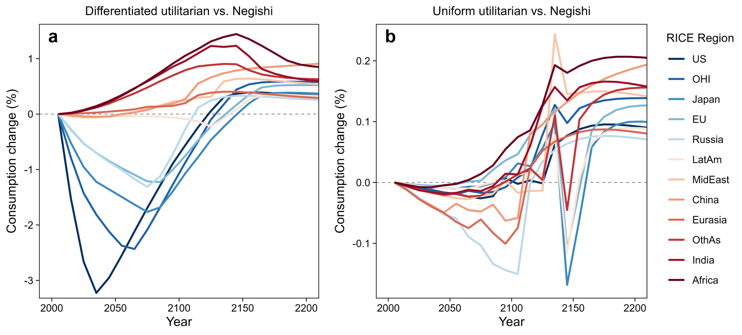
Figure A4: Relative regional consumption changes between the Negishi solution and the utilitarian solutions.

Notes: Consumption changes are percentage changes relative to the consumption level in the Negishi solution. Positive values indicate a higher consumption level in the utilitarian solutions. The figure shows the results for the utility discount rate of 1.5%.

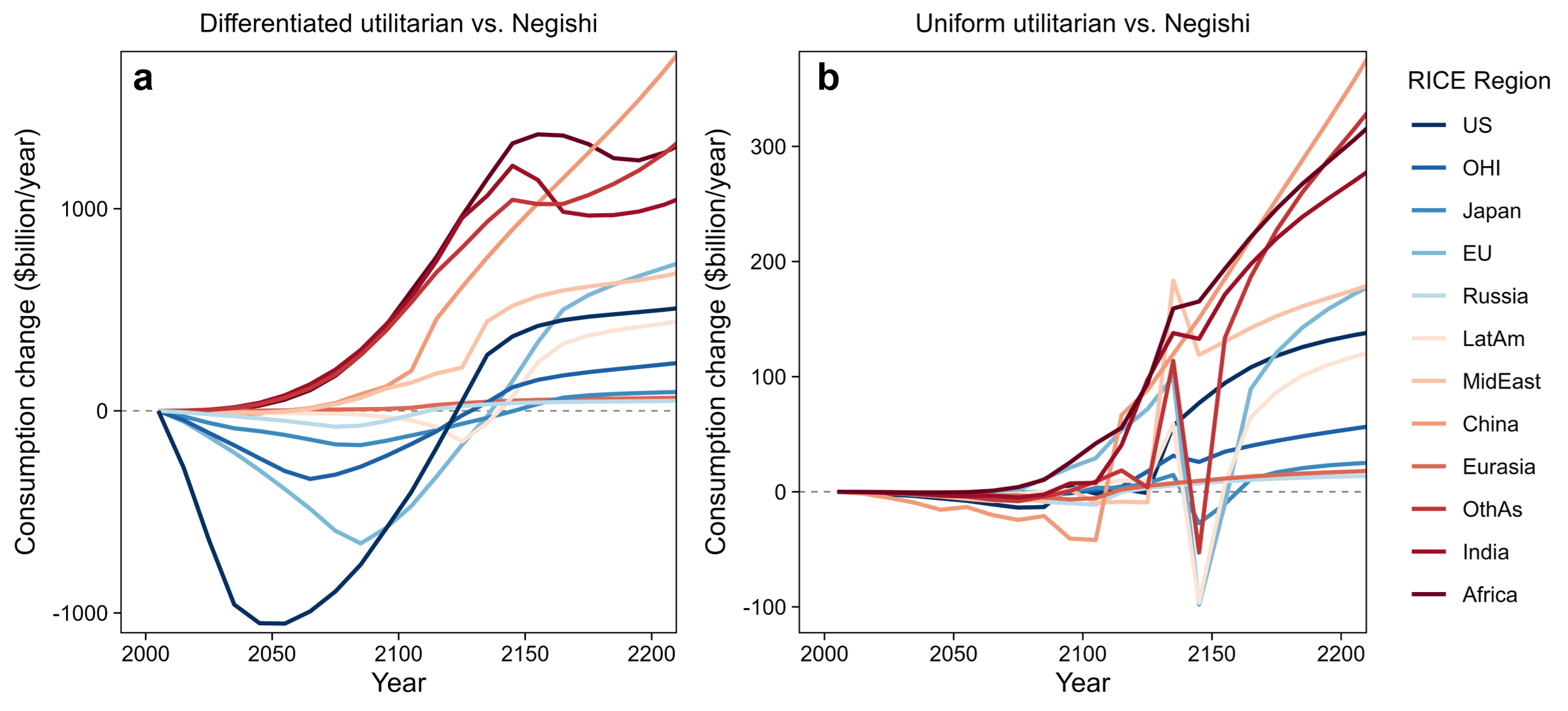
Figure A5: Regional consumption changes between the Negishi solution and the utilitarian solutions.

Notes: Positive values indicate a higher consumption level in the utilitarian solutions. The figure shows the results for the utility discount rate of 1.5%.

Notes: Consumption changes are percentage changes relative to the consumption level in the Negishi solution. Positive values indicate a higher consumption level in the utilitarian solutions. The figure shows the results for the utility discount rate of 0.1%.

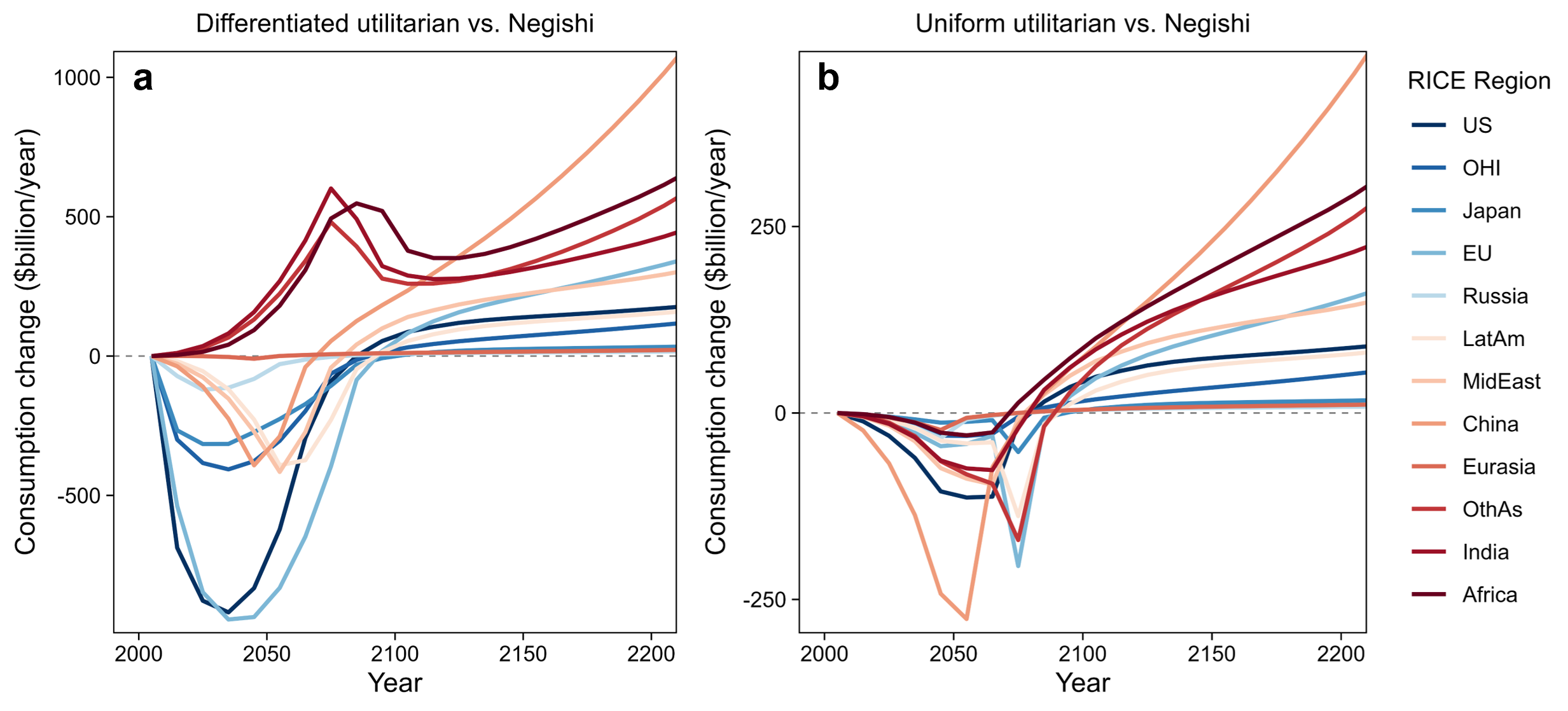
Figure A7: Regional consumption changes between the Negishi solution and the utilitarian solutions.

Notes: Positive values indicate a higher consumption level in the utilitarian solutions. The figure shows the results for the utility discount rate of 0.1%.

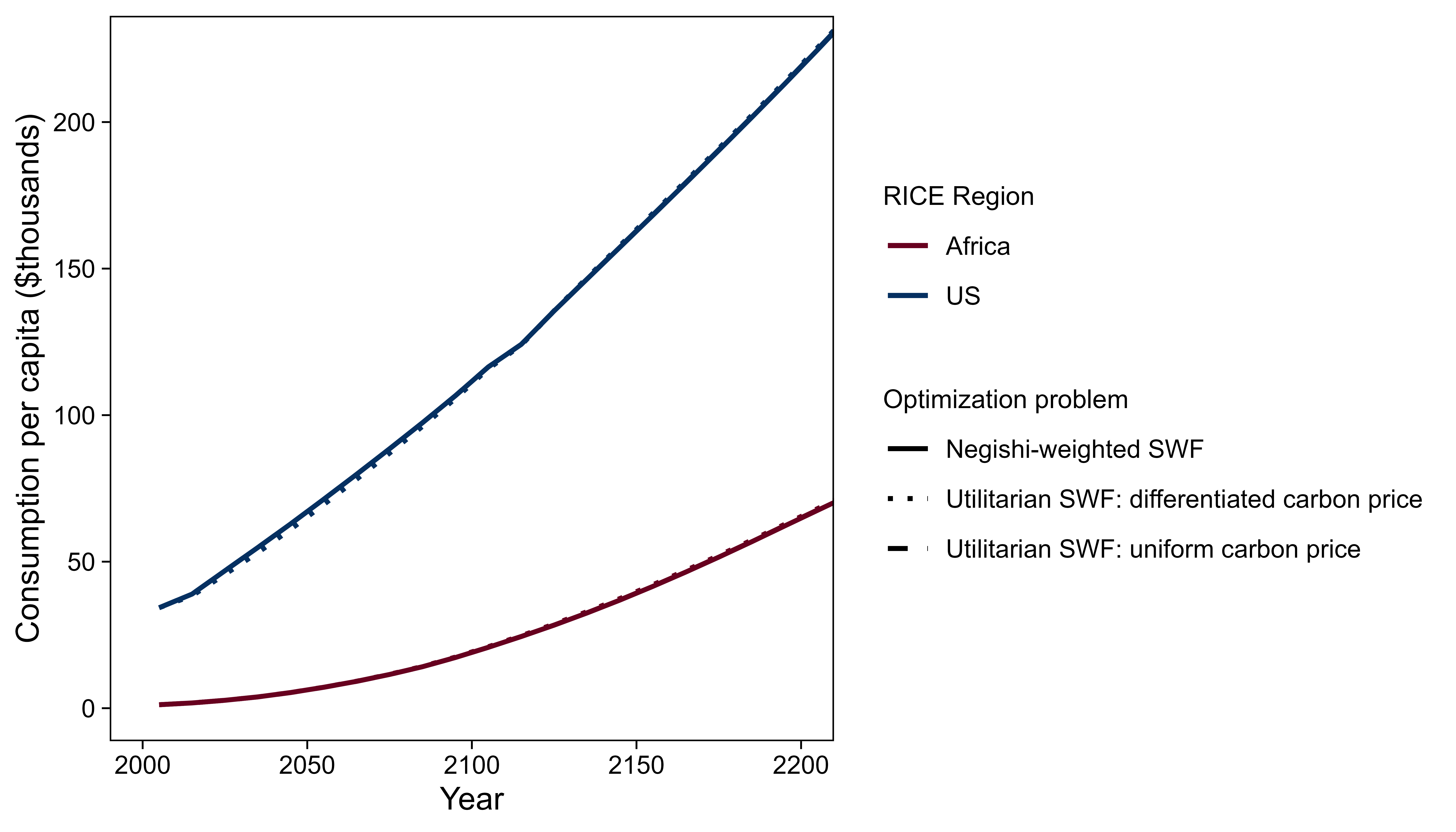
Figure A8: Consumption per capita trajectories for Africa and the US.

Notes: The figure shows the results for the utility discount rate of 1.5%.

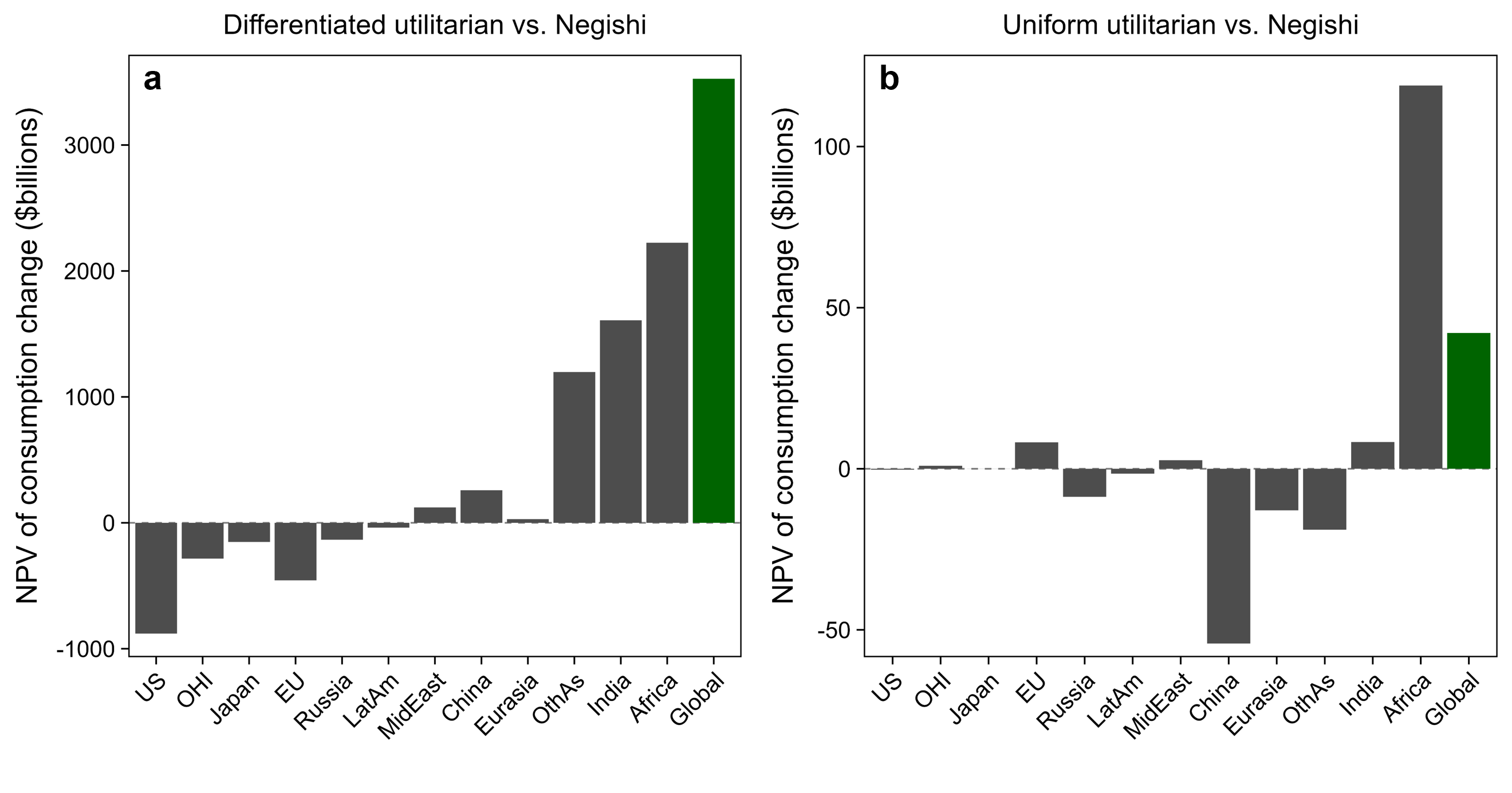
Figure A9: Utilitarian welfare changes.

Notes: The values express the regional and global utilitarian welfare change in the welfare-equivalent consumption change in 2005 if consumption were distributed equally (for details, see Appendix A.10). The figure shows the results for the utility discount rate of 1.5%.

Figure A10: Net present value of consumption changes.

Notes: The values show the welfare-equivalent consumption change in 2005, as a percentage of the consumption in 2005. The “Global” value expresses the global utilitarian welfare change in the welfare-equivalent consumption change in 2005 if consumption were distributed equally (for details, see Appendix A.10). The figure shows the results for the utility discount rate of 0.1%.

Figure A11: Utilitarian welfare changes.

Notes: The values express the regional and global utilitarian welfare change in the welfare-equivalent consumption change in 2005 if consumption were distributed equally (for details, see Appendix A.10). The figure shows the results for the utility discount rate of 0.1%.

Figure A12: Relative regional marginal damages, abatement cost convexities, population and economic growth.

Notes: The ratio of the convexities in the abatement cost functions is $c^{\prime\prime}_{i,2025}/c^{\prime\prime}_{US,2025}$ (evaluated at uniform carbon prices). The ratio of the marginal damages as a percentage of GDP is $d^{\prime}_{i,t}/d^{\prime}_{US,t}$. The ratios of population growth and economic growth are given by the relative growth factors $\frac{L_{i,t}/L_{i,2025}}{L_{US,t}/L_{US,2025}}$ and $\frac{y_{i,t}/y_{i,2025}}{y_{US,t}/y_{US,2025}}$. where $y$ is the GDP per capita. The year $t$ corresponds to either 2055, 2075, or 2095 in panels (a), (b), and (c), respectively. The figure shows the results for the utility discount rate of 1.5%.

Notes: The figure shows the results for the utility discount rate of 1.5%. Temperature changes are relative to 1900. Note that Russia, Eurasia and China have the lowest backstop technology prices, causing the large carbon price increases once it is beneficial for these regions to increase the globally uniform carbon price above the level of their respective backstop prices.

Appendix C: Supplementary Information

C.1 Optimal carbon prices for arbitrary welfare weights

Definition 7.

The optimal differentiated carbon price (for arbitrary welfare weights) for region $i$ is implicitly defined by

$$\tau_{i}^{diff}=C^{\prime}_{i}(A_{i}^{*})=-\frac{1}{\alpha_{i}u^{\prime}(x_{i}^{*})}\sum_{j\in\mathcal{I}}\alpha_{j}u^{\prime}(x_{j}^{*})D^{\prime}_{j}(A^{*}).$$ (A17)

In words, the optimal differentiated carbon price is equal to the sum of the avoided weighted marginal welfare damages divided by the weighted marginal utility. Thus, the optimal differentiated carbon price is inversely proportional to the weighted marginal utility, $\alpha_{i}u_{i}^{\prime}$. Consequently, the optimal differentiated carbon price is lower in the region with the higher weighted marginal utility. This result has first been established by [undefaj] and [undefw]. Note that, if the weighted marginal utilities are equal across regions (i.e., $\alpha_{S}u^{\prime}_{S}=\alpha_{N}u^{\prime}_{N}$), we obtain the knife-edge result that the optimal “differentiated” carbon price is in fact uniform. This is the case if the weights are the Negishi weights. I return to this below.

It is insightful to rearrange Equation (A17) to

$$\alpha_{i}u^{\prime}(x_{i}^{*})C^{\prime*}_{i}=-\sum_{j\in\mathcal{I}}\alpha_{j}u^{\prime}(x_{j}^{*})D^{\prime}_{j}(A^{*}).$$

Since the right-hand side is the same for all regions, we know that $\alpha_{N}u^{\prime}(x_{N}^{*})C^{\prime*}_{N}=\alpha_{S}u^{\prime}(x_{S}^{*})C^{\prime*}_{S}$. That is, the weighted marginal welfare cost of abatement (rather than the marginal abatement cost in monetary terms) is equalized across regions.

Definition 8.

The optimal uniform carbon price (for arbitrary welfare weights) is implicitly defined by

$$\tau^{uni}=C_{i}^{\prime}(A_{i}^{*})=-\sum_{i}\alpha_{i}u^{\prime}(x_{i}^{*})D^{\prime}_{i}(A^{*})\frac{C^{\prime\prime}_{S}+C^{\prime\prime}_{N}}{\alpha_{N}u^{\prime}(x_{N}^{*})C^{\prime\prime}_{S}+\alpha_{S}u^{\prime}(x_{S}^{*})C^{\prime\prime}_{N}}.$$ (A18)

The optimal uniform carbon price again depends on the sum of the avoided weighted marginal welfare damages. However, it also depends on a second factor which contains the second derivatives of the abatement cost functions. To gain some intuition, we can note that the expression collapses to the expression for the optimal differentiated carbon price if one of the regions has a linear abatement cost function; that is, $C^{\prime\prime}_{i}=0$ for one $i$. Specifically, if the Global North has a linear abatement cost function, then the expression collapses to the differentiated carbon price expression for the Global North; and vice-versa for the Global South. The intuition is that if one region has a linear abatement cost function, and thus constant marginal abatement costs, then the only way to equalize marginal abatement costs across regions is to adjust the marginal abatement cost of the other region. Unsurprisingly, this provides the intuition that the optimal uniform carbon price lies in between the two optimal differentiated prices. Moreover, whether the uniform carbon price is closer to one or the other differentiated carbon prices depends on the relative convexities of the abatement cost functions, the welfare weights, and the relative marginal utilities at the optimal solution.

C.2 Abatement cost and damage functions of the RICE model

In the RICE model, regional climate damages are given by

$$D_{it}=Y_{it}d_{it},$$

where $Y_{it}$ is the GDP gross of damages and abatement costs, and $d_{it}$ denotes the climate damage as a fraction of GDP, which is composed of damages from atmospheric temperature changes and sea level rise (which are ultimately functions of emissions/abatement).

Regional abatement costs are given by

$$C_{it}=Y_{it}\underbrace{\frac{b_{it}\sigma_{it}}{\theta}\left(\frac{A_{it}}{\sigma_{it}Y_{it}}\right)^{\theta}}_{c_{it}},$$

where $b_{it}$ is the price of a backstop technology (i.e., the marginal abatement cost at which emissions can be abated completely), $\sigma_{it}$ is the baseline emissions intensity (emissions per GDP) of the economy in the absence of abatement, $\theta>1$ is a parameter that governs the convexity of the abatement cost function (in RICE, $\theta=2.8$). Note that the abatement costs per GDP, $c_{it}$, are a function of $\frac{A_{it}}{Y_{it}}$.

The damage function from atmospheric temperature changes is shown in Figure A14. The trajectories of the regional baseline carbon intensities and backstop technology prices are shown in Figure A15.

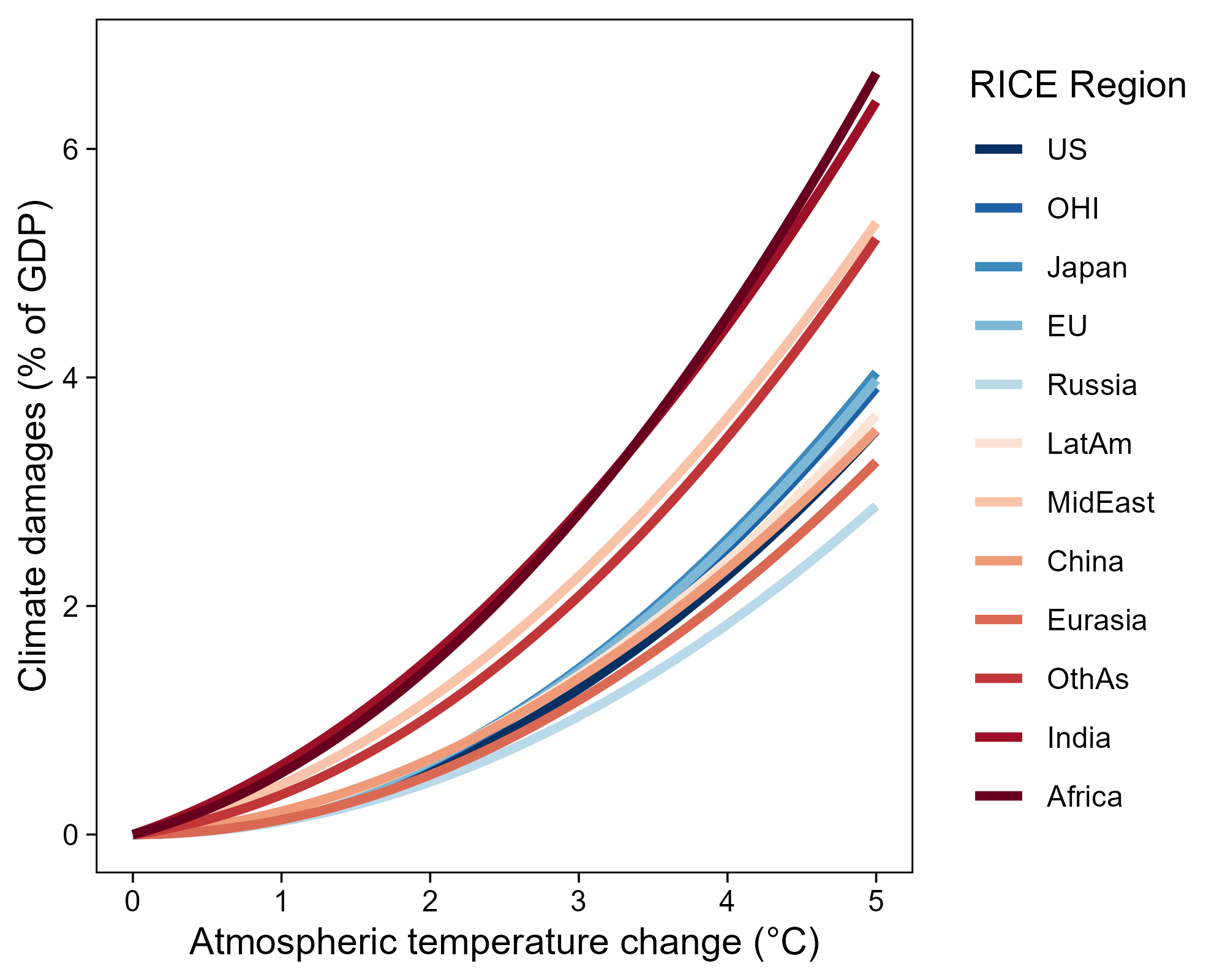
Figure A14: Regional damage functions for atmospheric temperature changes in the RICE model.

Notes: Temperature changes are relative to temperatures in 1900.

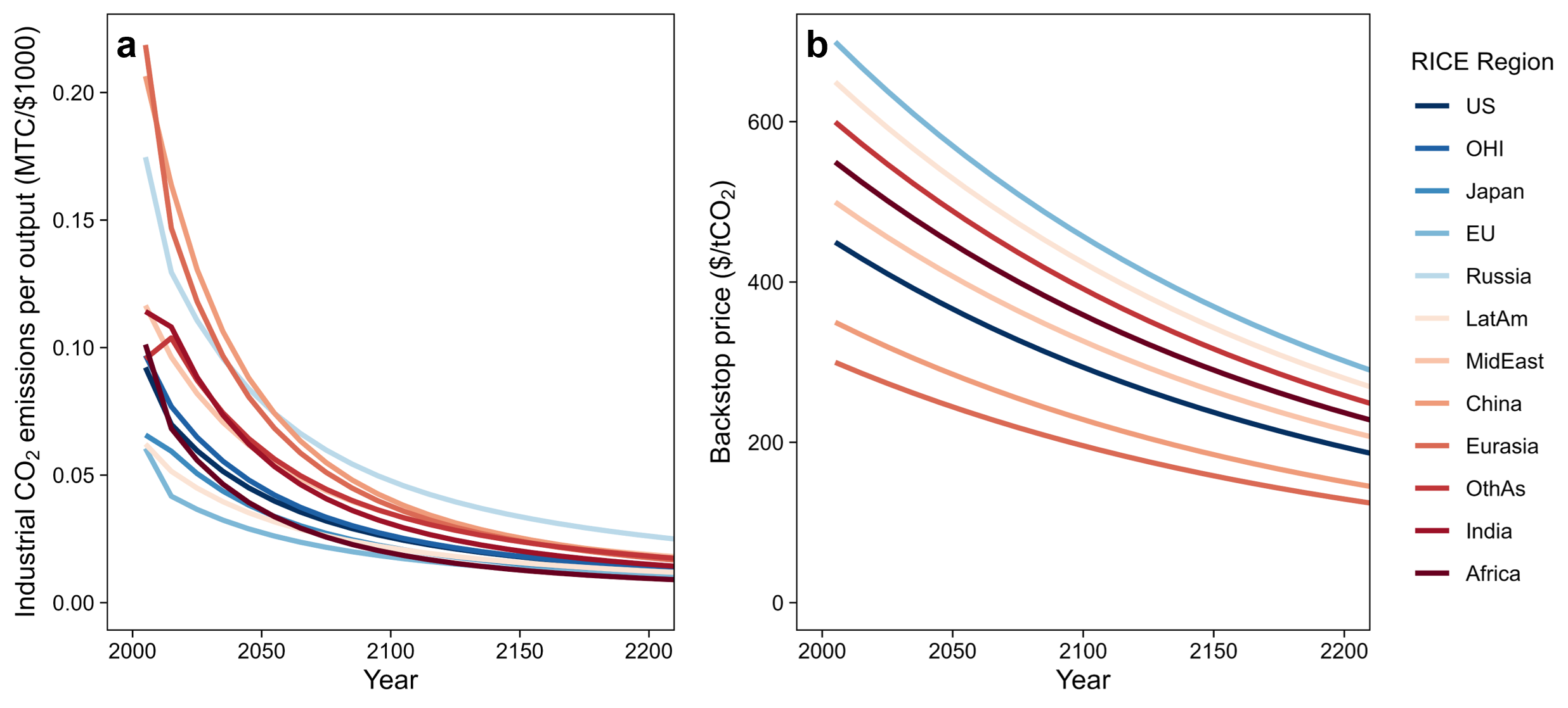
Figure A15: Regional baseline carbon intensities (a) and backstop technology prices (b) in the RICE model.

Notes: The carbon intensity is given by the industrial CO₂ emissions per economic output. The backstop technology price corresponds to the marginal abatement cost at which all emissions are abated. The following regions have identical backstop prices: (1) Russia and Eurasia, (2) Other High Income (OHI) countries, Africa, and India, (3) Japan and the EU.

C.3 Time-variant Negishi weights

The time-variant Negishi welfare weights are given by

$$\alpha_{it}=\frac{1}{u^{\prime}\left(x_{it}\right)}v_{t},$$

where $v_{t}$ is the wealth-based component of the social discount factor. In the RICE-2010 model [undefaaf], it is defined as the capital-weighted average of the regional wealth-based discount factors:

$$\begin{aligned} v_{t}&=\frac{u^{\prime}_{US,t}}{u^{\prime}_{US,0}}\sqrt{\frac{\sum_{i\in\mathscr{I}}\left(\frac{{\frac{u^{\prime}_{US,0}}{u^{\prime}_{i0}}}}{\frac{u^{\prime}_{US,t}}{u^{\prime}_{it}}}\frac{K_{it}}{\sum_{j\in\mathscr{I}}K_{jt}}\right)}{\sum_{i\in\mathscr{I}}\left(\frac{\frac{u^{\prime}_{US,t}}{u^{\prime}_{it}}}{\frac{u^{\prime}_{US,0}}{u^{\prime}_{i0}}}\frac{K_{it}}{\sum_{j\in\mathscr{I}}K_{jt}}\right)}},\end{aligned}$$

where $K_{it}$ is the capital stock.

Note that $\frac{1}{u^{\prime}(x_{it})}v_{t}$ equalizes the weighted marginal utility across regions. To obtain equalized weighted marginal utilities in each period, the discount factor needs to be equal across regions. Thus, $v_{t}$ is not region-specific and it pins down the wealth-based component of the world discount factor [undefaal].

C.4 Discussion of the differentiated carbon price optimum

The welfare maximizing policy that allows for differentiated carbon prices requires much higher carbon prices in rich regions than in poor regions (see Figure A2 and Table 3). This result warrants a discussion of several issues.

First, the differentiated carbon price optimum may be opposed by rich nations as it results in an implicit transfer from rich to poor regions. It should be noted, however, that the uniform carbon price optimum is welfare inferior to the differentiated carbon price optimum, as it imposes an additional constraint [undefp]. Importantly, the differentiated carbon price optimum is also in accordance with the principle of “common but differentiated responsibilities and respective capabilities” of the United Nations Framework Convention on Climate Change [undefaaae]. As such, [undefp] argue that the differentiated carbon price optimum is a natural focal point for international climate policy and for evaluating the adequacy of the nationally determined contributions (NDCs), which are at the heart of the Paris Agreement. A more recent study by [undefr] provides this comparison of the NDCs to implied carbon budgets under the differentiated carbon price optimum.

Second, since differentiated carbon prices are not cost-effective, it should be reemphasized that a further welfare improvement over the differentiated price optimum could be achieved by establishing an international emissions trading scheme. This would allow regions with higher carbon prices to buy emission permits from poorer regions where the carbon price is lower, implying a transfer from the rich to the poor. Due to the differential carbon prices, mutual gains can be achieved by such a trading scheme [undefp]. If the permit market is fully competitive, this would result in a globally harmonized carbon price. However, as [undefp] point out, this outcome would be different from the uniform carbon price optimum discussed above, where an a priori constraint of equalized carbon prices was imposed; total emissions will be reduced and the poorest countries will bear a lower burden under the harmonized carbon price attained by the emissions trading scheme. [undefw] thus propose that the efficient allocation of emission permits is established by the differentiated carbon price optimum, and once the optimal allocation of permits is found, these permits are then traded internationally to achieve further welfare gains. The emission budgets shown in Figure A2 can thus be understood as providing the first step of this process.

Third, a potential problem with differentiated carbon prices is carbon leakage – an increase in carbon emissions in a country with comparatively laxer climate policies as a result of stricter climate policies in another country (e.g., due to a relocation of carbon-intensive industries to countries with laxer climate policies). The problem of carbon leakage, if it is not addressed, may thus undermine the policy. [undefr] provide a brief discussion of the issue of carbon leakage and how it may be addressed. They note that there are two channels for carbon leakage: (1) competitiveness differences resulting from carbon price differences, and (2) lower fossil fuel prices due to decreased global demand. [undefr] argue that the competitiveness channel can be addressed with border tax adjustments, such as those proposed by [undefak]. The second channel is shut down if countries commit to a global emissions cap [undefr]. Of course, there is also no carbon leakage if each region commits to its own regional carbon budget.

References

- [undef] Joshua K Abbott and Eli P Fenichel “Following the golden rule: Negishi welfare weights without apology” ++ In Arizona State University & Yale University, 2014
- [undefa] Matthew Adler, David Anthoff, Valentina Bosetti, Greg Garner, Klaus Keller and Nicolas Treich “Priority for the worse-off and the social cost of carbon” ++ In Nature Climate Change 7.6, 2017, pp. 443
- [undefb] David Anthoff “Optimal Global Dynamic Carbon Abatement” Job Market Paper, 2011 URL: https://www.david-anthoff.com/AnthoffJobmarketPaper.pdf
- [undefc] David Anthoff, Francis Dennig and Johannes Emmerling “On Differentiated Carbon Prices and Discount Rates”, 2021 URL: https://papers.ssrn.com/abstract=3906413
- [undefd] David Anthoff and Johannes Emmerling “Inequality and the Social Cost of Carbon” ++ In Journal of the Association of Environmental and Resource Economists 6.2, 2018, pp. 29–59 DOI: 10.1086/701900
- [undefe] David Anthoff, Frank Errickson and Lisa Rennels “Mimi-RICE-2010.jl - a julia implementation of the RICE 2010 model” Berkeley, CA, United States: The Society, EnvironmentEconomics Lab, 2019 URL: https://github.com/anthofflab/mimi-rice-2010.jl
- [undeff] David Anthoff, Cameron Hepburn and Richard S.. Tol “Equity weighting and the marginal damage costs of climate change” In Ecological Economics 68.3, 2009, pp. 836–849 DOI: 10.1016/j.ecolecon.2008.06.017
- [undefg] Kenneth J. Arrow, Maureen Cropper, Christian Gollier, Ben Groom, Geoffrey M. Heal, Richard G. Newell, William D. Nordhaus, Robert S. Pindyck, William A. Pizer, Paul Portney, Thomas Sterner, Richard S.. Tol and Martin Weitzman “How Should Benefits and Costs Be Discounted in an Intergenerational Context? The Views of an Expert Panel”, 2013 URL: https://papers.ssrn.com/abstract=2199511
- [undefh] C. Azar and T. Sterner “Discounting and distributional considerations in the context of global warming” + In Ecological Economics 19.2, 1996, pp. 169–184 DOI: 10.1016/0921-8009(96)00065-1
- [undefi] Lint Barrage “Optimal Dynamic Carbon Taxes in a Climate–Economy Model with Distortionary Fiscal Policy” In The Review of Economic Studies 87.1, 2020, pp. 1–39 DOI: 10.1093/restud/rdz055
- [undefj] Wilfred Beckerman and Cameron Hepburn “Ethics of the Discount Rate in the Stern Review on the Economics of Climate Change” ++, 2007, pp. 26
- [undefk] Abram Bergson “A Reformulation of Certain Aspects of Welfare Economics” In The Quarterly Journal of Economics 52.2, 1938, pp. 310–334 DOI: 10.2307/1881737
- [undefl] E.. Birgin and J.. Martínez “Improving ultimate convergence of an augmented Lagrangian method” In Optimization Methods and Software 23, 2008
- [undefm] Kirill Borissov and Lucas Bretschger “Optimal carbon policies in a dynamic heterogeneous world” In European Economic Review 148, 2022, pp. 104253 DOI: 10.1016/j.euroecorev.2022.104253
- [undefn] Valentina Bosetti, Carlo Carraro, Enrica De Cian, Emanuele Massetti and Massimo Tavoni “Incentives and Stability of International Climate Coalitions: An Integrated Assessment”, 2012 DOI: 10.2139/ssrn.1991775
- [undefo] Lucas Bretschger “Climate policy and equity principles: fair burden sharing in a dynamic world” Publisher: Cambridge University Press In Environment and Development Economics 18.5, 2013, pp. 517–536 DOI: 10.1017/S1355770X13000284
- [undefp] Mark Budolfson and Francis Dennig “Optimal global climate policy and regional carbon prices” In Handbook on the Economics of Climate Change Edward Elgar Publishing, 2020, pp. 224–238
- [undefq] Mark Budolfson, Francis Dennig, Marc Fleurbaey, Noah Scovronick, Asher Siebert, Dean Spears and Fabian Wagner “Optimal Climate Policy and the Future of World Economic Development” ++ In The World Bank Economic Review, 2018 DOI: 10.1093/wber/lhx016
- [undefr] Mark B. Budolfson, David Anthoff, Francis Dennig, Frank Errickson, Kevin Kuruc, Dean Spears and Navroz K. Dubash “Utilitarian benchmarks for emissions and pledges promote equity, climate and development” +++ In Nature Climate Change, 2021, pp. 1–7 DOI: 10.1038/s41558-021-01130-6
- [undefs] Marshall Burke, Solomon M. Hsiang and Edward Miguel “Global non-linear effect of temperature on economic production” +++ In Nature 527.7577, 2015, pp. 235–239 DOI: 10.1038/nature15725
- [undeft] Tamma Carleton, Amir Jina, Michael Delgado, Michael Greenstone, Trevor Houser, Solomon Hsiang, Andrew Hultgren, Robert E Kopp, Kelly E McCusker, Ishan Nath, James Rising, Ashwin Rode, Hee Kwon Seo, Arvid Viaene, Jiacan Yuan and Alice Tianbo Zhang “Valuing the Global Mortality Consequences of Climate Change Accounting for Adaptation Costs and Benefits*” In The Quarterly Journal of Economics, 2022, pp. qjac020 DOI: 10.1093/qje/qjac020
- [undefu] Lucas Chancel, Philipp Bothe and Tancrède Voituriez “Climate Inequality Report: Fair Taxes for a Sustainable Future in the Global South” Publisher: WIL: World Inequality Lab, 2023 URL: https://policycommons.net/artifacts/3441273/cbv2023-climateinequalityreport1/4241244/
- [undefv] Kiran Chawla “Normative Challenges in Climate Change Economics” In Handbook of the Philosophy of Climate Change Cham: Springer International Publishing, 2023, pp. 249–266 DOI: 10.1007/978-3-031-07002-0˙17
- [undefw] Graciela Chichilnisky and Geoffrey Heal “Who should abate carbon emissions?: An international viewpoint” In Economics Letters 44.4, 1994, pp. 443–449 DOI: 10.1016/0165-1765(94)90119-8
- [undefx] “Environmental Markets: Equity and Efficiency” Columbia University Press, 2000 DOI: 10.7312/chic11588
- [undefy] Graciela Chichilnisky, Geoffrey Heal and David Starrett “Equity and efficiency in environmental markets: global trade in carbon dioxide emissions” ++ In Environmental markets: equity and efficiency 15, 2000
- [undefz] undef Climate Watch “Explore Nationally Determined Contributions (NDCs)” Washington, DC: World Resources Institute, 2022 URL: https://www.climatewatchdata.org
- [undefaa] Antoine d’Autume, Katheline Schubert and Cees Withagen “Should the Carbon Price Be the Same in All Countries?” _eprint: https://onlinelibrary.wiley.com/doi/pdf/10.1111/jpet.12162 In Journal of Public Economic Theory 18.5, 2016, pp. 709–725 DOI: 10.1111/jpet.12162
- [undefab] Partha Dasgupta “Discounting climate change” In Journal of Risk and Uncertainty 37.2, 2008, pp. 141–169 DOI: 10.1007/s11166-008-9049-6
- [undefac] Francis Dennig, David Anthoff, Frank Errickson and Lisa Rennels “RICEupdate” original-date: 2019-12-10T10:30:31Z, 2019 URL: https://github.com/fdennig/RICEupdate
- [undefad] Francis Dennig, Mark B. Budolfson, Marc Fleurbaey, Asher Siebert and Robert H. Socolow “Inequality, climate impacts on the future poor, and carbon prices” +++ In Proceedings of the National Academy of Sciences, 2015, pp. 201513967 DOI: 10.1073/pnas.1513967112
- [undefae] Francis Dennig and Johannes Emmerling “A Note on Optima with Negishi Weights” In Working Paper, 2017
- [undefaf] Francis Dennig and Johannes Emmerling “A note on optima with time-varying Negishi weights” ++ In Working Paper, 2019
- [undefag] Francis Dennig, Frank Errickson and David Anthoff “mimi_NICE” original-date: 2017-06-26T11:08:07Z, 2017 URL: https://github.com/fdennig/mimi_NICE
- [undefah] Simon Dietz and Nicholas Stern “Why Economic Analysis Supports Strong Action on Climate Change: A Response to the Stern Review’s Critics” + In Review of Environmental Economics and Policy 2.1, 2008, pp. 94–113 DOI: 10.1093/reep/ren001
- [undefai] Thomas Douenne, Albert Jan Hummel and Marcelo Pedroni “Optimal Fiscal Policy in a Climate-Economy Model with Heterogeneous Households” Rochester, NY: Social Science Research Network, 2023 DOI: 10.2139/ssrn.4018468
- [undefaj] Johan Eyckmans, Stef Proost and Erik Schokkaert “Efficiency and distribution in greenhouse negotiations” Publisher: Ashgate Pub Ltd In The Economics of International Environmental Agreements, 1993, pp. 157
- [undefak] Brian Flannery, Jennifer Hillman, Jan Mares and Matthew C. Porterfield “Framework Proposal for a US Upstream Greenhouse Gas Tax with WTO-Compliant Border Adjustments”, 2018 URL: https://papers.ssrn.com/abstract=3148213
- [undefal] Marc Fleurbaey and François Maniquet “Utilitarianism versus fairness in welfare economics” In Justice, Political Liberalism, and Utilitarianism: Themes from Harsanyi and Rawls, 2008, pp. 263–280 DOI: 10.1017/CBO9780511619595.012
- [undefam] Marc Fleurbaey and François Maniquet “Optimal Income Taxation Theory and Principles of Fairness” In Journal of Economic Literature 56.3, 2018, pp. 1029–1079 DOI: 10.1257/jel.20171238
- [undefan] Paolo Gazzotti, Johannes Emmerling, Giacomo Marangoni, Andrea Castelletti, Kaj-Ivar van der Wijst, Andries Hof and Massimo Tavoni “Persistent inequality in economically optimal climate policies” Number: 1 Publisher: Nature Publishing Group In Nature Communications 12.1, 2021, pp. 3421 DOI: 10.1038/s41467-021-23613-y
- [undefao] Christian Gollier “The Debate on Discounting: Reconciling Positivists and Ethicists” In Chicago Journal of International Law, 2012, pp. 549–564 URL: https://heinonline.org/HOL/P?h=hein.journals/cjil13&i=555
- [undefap] Christian Gollier “Discounting, inequality and economic convergence” In Journal of Environmental Economics and Management 69, 2015, pp. 53–61 DOI: 10.1016/j.jeem.2014.10.005
- [undefaq] Mikhail Golosov, John Hassler, Per Krusell and Aleh Tsyvinski “Optimal Taxes on Fossil Fuel in General Equilibrium” _eprint: https://onlinelibrary.wiley.com/doi/pdf/10.3982/ECTA10217 In Econometrica 82.1, 2014, pp. 41–88 DOI: https://doi.org/10.3982/ECTA10217
- [undefar] John C. Harsanyi “Cardinal Welfare, Individualistic Ethics, and Interpersonal Comparisons of Utility” In Journal of Political Economy 63.4, 1955, pp. 309–321 URL: https://www.jstor.org/stable/1827128
- [undefas] Steven G. Johnson “The NLopt nonlinear-optimization package”, 2020 URL: http://github.com/stevengj/nlopt
- [undefat] Matthias Kalkuhl and Leonie Wenz “The impact of climate conditions on economic production. Evidence from a global panel of regions” In Journal of Environmental Economics and Management 103, 2020, pp. 102360 DOI: 10.1016/j.jeem.2020.102360
- [undefau] J. Kelleher “Reflections on the 2018 Nobel Memorial Prize Awarded to William Nordhaus” In Erasmus Journal for Philosophy and Economics 12(1), 2019, pp. 93–107
- [undefav] Ulrike Kornek, David Klenert, Ottmar Edenhofer and Marc Fleurbaey “The social cost of carbon and inequality: When local redistribution shapes global carbon prices” In Journal of Environmental Economics and Management 107, 2021, pp. 102450 DOI: 10.1016/j.jeem.2021.102450
- [undefaw] Matthew J. Kotchen “Which Social Cost of Carbon? A Theoretical Perspective” +++ In Journal of the Association of Environmental and Resource Economists 5.3, 2018, pp. 673–694 DOI: 10.1086/697241
- [undefax] Marian Leimbach, Nico Bauer, Lavinia Baumstark and Ottmar Edenhofer “Mitigation Costs in a Globalized World: Climate Policy Analysis with REMIND-R” In Environmental Modeling & Assessment 15.3, 2010, pp. 155–173 DOI: 10.1007/s10666-009-9204-8
- [undefay] Humberto Llavador, John E. Roemer and Joaquim Silvestre “Intergenerational justice when future worlds are uncertain” In Journal of Mathematical Economics 46.5, Mathematical Economics: Special Issue in honour of Andreu Mas-Colell, Part 1, 2010, pp. 728–761 DOI: 10.1016/j.jmateco.2010.06.004
- [undefaz] Humberto Llavador, John E. Roemer and Joaquim Silvestre ““A dynamic analysis of human welfare in a warming planet”” In Journal of Public Economics 95.11, Special Issue: International Seminar for Public Economics on Normative Tax Theory, 2011, pp. 1607–1620 DOI: 10.1016/j.jpubeco.2011.05.017
- [undefaaa] Alan S. Manne and Richard G. Richels “Merge: An Integrated Assessment Model for Global Climate Change” In Energy and Environment New York: Springer-Verlag, 2005, pp. 175–189 DOI: 10.1007/0-387-25352-1˙7
- [undefaab] Andreu Mas-Colell, Michael Dennis Whinston and Jerry R Green “Microeconomic theory” Oxford university press New York, 1995
- [undefaac] Aurélie Méjean, Peron Collins-Sowah, Céline Guivarch, Franziska Piontek, Bjoern Soergel and Nicolas Taconet “Climate change impacts increase economic inequality: evidence from a systematic literature review” Publisher: IOP Publishing In Environmental Research Letters 19.4, 2024, pp. 043003 DOI: 10.1088/1748-9326/ad376e
- [undefaad] J.. Mirrlees “An Exploration in the Theory of Optimum Income Taxation” Publisher: [Oxford University Press, Review of Economic Studies, Ltd.] In The Review of Economic Studies 38.2, 1971, pp. 175–208 DOI: 10.2307/2296779
- [undefaae] Takashi Negishi “Welfare Economics and Existence of an Equilibrium for a Competitive Economy” _eprint: https://onlinelibrary.wiley.com/doi/pdf/10.1111/j.1467-999X.1960.tb00275.x In Metroeconomica 12.2, 1960, pp. 92–97 DOI: 10.1111/j.1467-999X.1960.tb00275.x
- [undefaaf] William Nordhaus “Economic aspects of global warming in a post-Copenhagen environment” In Proceedings of the National Academy of Sciences 107.26, 2010, pp. 11721–11726 DOI: 10.1073/pnas.1005985107
- [undefaag] William Nordhaus “Estimates of the Social Cost of Carbon: Background and Results from the RICE-2011 Model”, 2011 URL: http://www.nber.org/papers/w17540
- [undefaah] William Nordhaus “Integrated Economic and Climate Modeling” In Handbook of Computable General Equilibrium Modeling 1, Handbook of Computable General Equilibrium Modeling SET, Vols. 1A and 1B Elsevier, 2013, pp. 1069–1131 DOI: 10.1016/B978-0-444-59568-3.00016-X
- [undefaai] William Nordhaus and Paul Sztorc “DICE 2013R: Introduction and user’s manual”, 2013
- [undefaaj] William Nordhaus and Zili Yang “A Regional Dynamic General-Equilibrium Model of Alternative Climate-Change Strategies” In The American Economic Review 86.4, 1996, pp. 741–765 URL: https://www.jstor.org/stable/2118303
- [undefaak] William D Nordhaus “A Review of the Stern Review on the Economics of Climate Change” In Journal of Economic Literature, 2007, pp. 49
- [undefaal] William D Nordhaus and Joseph Boyer “Warming the world: economic models of global warming” MIT press, 2000
- [undefaam] Thomas Piketty and Emmanuel Saez “Optimal Labor Income Taxation” In Handbook of Public Economics 5, handbook of public economics, vol. 5 Elsevier, 2013, pp. 391–474 DOI: 10.1016/B978-0-444-53759-1.00007-8
- [undefaan] Brian C. Prest, Lisa Rennels, Frank Errickson and David Anthoff “Equity weighting increases the social cost of carbon” Publisher: American Association for the Advancement of Science In Science 385.6710, 2024, pp. 715–717 DOI: 10.1126/science.adn1488
- [undefaao] Narasimha D. Rao “International and intranational equity in sharing climate change mitigation burdens” In International Environmental Agreements: Politics, Law and Economics 14.2, 2014, pp. 129–146 DOI: 10.1007/s10784-013-9212-7
- [undefaap] Lionel Charles Robbins Robbins “An essay on the nature & significance of economic science.”, 1935
- [undefaaq] John E. Roemer “The Ethics of Intertemporal Distribution in a Warming Planet” In Environmental and Resource Economics 48.3, 2011, pp. 363–390 DOI: 10.1007/s10640-010-9414-1
- [undefaar] Thomas H. Rowan “Functional Stability Analysis of Numerical Algorithms”, 1990
- [undefaas] Paul A. Samuelson “The Pure Theory of Public Expenditure” Publisher: The MIT Press In The Review of Economics and Statistics 36.4, 1954, pp. 387–389 DOI: 10.2307/1925895
- [undefaat] Paul Anthony Samuelson “Foundations of economic analysis” Cambridge: Harvard University Press, 1947
- [undefaau] Agnar Sandmo “Global public economics: Public goods and externalities” ++ In Économie publique/Public economics, 2007
- [undefaav] Ingmar Schumacher “The aggregation dilemma in climate change policy evaluation” + In Climate Change Economics 09.3, 2018, pp. 1850008 DOI: 10.1142/S2010007818500082
- [undefaaw] Amartya Sen “Interpersonal Aggregation and Partial Comparability” In Econometrica 38.3, 1970, pp. 393–409 DOI: 10.2307/1909546
- [undefaax] Amartya Sen “The Moral Standing of the Market” Publisher: Cambridge University Press In Social Philosophy and Policy 2.2, 1985, pp. 1–19 DOI: 10.1017/S0265052500003186
- [undefaay] Leslie Shiell “Equity and efficiency in international markets for pollution permits” In Journal of Environmental Economics and Management 46.1, 2003, pp. 38–51 DOI: 10.1016/S0095-0696(02)00028-1
- [undefaaz] Elizabeth A Stanton “Negishi welfare weights in integrated assessment models: the mathematics of global inequality” In Climatic Change 107.3, 2011, pp. 417–432
- [undefaaaa] Elizabeth A Stanton, Frank Ackerman and Sivan Kartha “Inside the integrated assessment models: Four issues in climate economics” In Climate and Development 1.2, 2009, pp. 166–184
- [undefaaab] Nicholas Stern, Siobhan Peters, Vicki Bakhshi, Alex Bowen, Catherine Cameron, Sebastian Catovsky, Diane Crane, Sophie Cruickshank, Simon Dietz and Nicola Edmonson “Stern Review: The economics of climate change” HM treasury London, 2006
- [undefaaac] Nicholas Herbert Stern “The Economics of Climate Change: The Stern Review” Cambridge, UK: Cambridge University Press, 2007
- [undefaaad] Joseph E. Stiglitz “Pareto efficient and optimal taxation and the new new welfare economics” In Handbook of Public Economics 2 Elsevier, 1987, pp. 991–1042 DOI: 10.1016/S1573-4420(87)80010-1
- [undefaaae] undef UNFCCC “United Nations framework convention on climate change” UNFCCC New York, 1992
- [undefaaaf] undef UNFCCC “Report of the Conference of the Parties on its twenty-first session, held in Paris from 30 November to 13 December 2015 Addendum Contents Part two: Action taken by the Conference of the Parties at its twenty-first session, Decision 1/CP.21 Adoption of the Paris Agreement.”, 2015
- [undefaaag] undef US Office of Management and Budget “Circular No. A-4”, 2023
- [undefaaah] Martin L. Weitzman “Can Negotiating a Uniform Carbon Price Help to Internalize the Global Warming Externality?” Publisher: The University of Chicago Press In Journal of the Association of Environmental and Resource Economists 1.1, 2014, pp. 29–49 DOI: 10.1086/676039
- [undefaaai] Martin L. Weitzman “On a World Climate Assembly and the Social Cost of Carbon” _eprint: https://onlinelibrary.wiley.com/doi/pdf/10.1111/ecca.12248 In Economica 84.336, 2017, pp. 559–586 DOI: 10.1111/ecca.12248
- [undefaaaj] Martin L. Weitzman “Voting on prices vs. voting on quantities in a World Climate Assembly” In Research in Economics 71.2, 2017, pp. 199–211 DOI: 10.1016/j.rie.2016.10.004
- [undefaaak] undef World Bank “State and Trends of Carbon Pricing 2023”, 2023 DOI: 10.1596/39796
- [undefaaal] undef World Bank “World Bank Open Data. GDP deflator: linked series (base year varies by country) - United States”, 2023 URL: https://data.worldbank.org/indicator/NY.GDP.DEFL.ZS.AD?locations=US
- [undefaaam] undef World Economics “Global South”, 2024 URL: https://www.worldeconomics.com/Regions/Global-South/default.aspx
- [undefaaan] Zili Yang and William D. Nordhaus “Magnitude and direction of technological transfers for mitigating GHG emissions” In Energy Economics 28.5, Modeling Technological Change in Climate Policy Analyses, 2006, pp. 730–741 DOI: 10.1016/j.eneco.2006.05.015