Higgs-like inflation in scalar-torsion $f(T,\phi)$ gravity in light of ACT-SPT-DESI constraints

Abstract

We study Higgs-like inflation in the framework of scalar-torsion gravity, focusing on the general class of $f(T,\phi)$ theories in which gravitation is mediated by torsion rather than curvature. Motivated by the increasing precision of cosmic microwave background and large-scale-structure observations, we examine whether Higgs-like inflation remains compatible with current data in this extended gravitational setting. Working within the slow-roll approximation, we analyze the inflationary dynamics both analytically and numerically. In the dominant-coupling regime we derive closed-form expressions for the scalar spectral index and the tensor-to-scalar ratio as functions of the number of e-folds, and we subsequently relax this assumption by numerically solving the slow-roll equations. Confrontation with the latest constraints from Planck 2018, ACT DR6, DESI DR1, and BICEP/Keck shows that Higgs-like inflation in $f(T,\phi)$ gravity is fully consistent with current bounds, naturally accommodating the preferred shift in the scalar spectral index and leading to distinctive tensor-sector signatures.

I Introduction

The inflationary paradigm, which is based on a brief period of accelerated expansion preceding the standard Hot Big Bang evolution, constitutes one of the cornerstones of modern cosmology. This early phase of quasi-exponential expansion provides a compelling resolution to several conceptual problems of the standard cosmological model, including the flatness, horizon, and monopole problems Starobinsky; Guth:1980zm; Albrecht:1982wi; Linde:1981mu. Moreover, inflation offers a natural mechanism for generating the primordial inhomogeneities that seeded the cosmic microwave background (CMB) anisotropies and the formation of large-scale structure (LSS). These inhomogeneities are believed to originate from quantum fluctuations amplified to cosmological scales during inflation, resulting in a nearly scale-invariant, adiabatic, and Gaussian spectrum of curvature perturbations Weinberg:2008zzc; Baumann:2018muz.

A key observational probe of inflationary dynamics is the scalar spectral index $n_{s}$, which characterizes the scale dependence of the primordial curvature power spectrum. The Planck 2018 analysis reported $n_{s}=0.9649\pm 0.0042$ (68% C.L.) Planck:2018jri, together with an upper bound on the tensor-to-scalar ratio, $r_{0.05}<0.036$, from BICEP/Keck BICEPKeck:2021gln. More recent high-precision measurements have further sharpened these constraints. The combination of Planck with South Pole Telescope (SPT) data yields $n_{s}=0.9647\pm 0.0037$ SPT-3G:2024atg, while the latest Atacama Cosmology Telescope (ACT) results combined with Planck shift the preferred value upward to $n_{s}=0.9709\pm 0.0038$ AtacamaCosmologyTelescope:2025blo; AtacamaCosmologyTelescope:2025nti. Including DESI DR1 large-scale structure data further tightens the constraint to $n_{s}=0.9743\pm 0.0034$ AtacamaCosmologyTelescope:2025blo, notably closer to exact scale invariance. This steady improvement in precision reveals the increasing distinguishing power of current and upcoming cosmological surveys.

Beyond the standard observables $n_{s}$ and $r$, inflation generically predicts additional signatures. A stochastic background of primordial gravitational waves (PGWs), if detected, would provide a direct window into the energy scale of inflation and the quantum nature of gravity in the early Universe Kamionkowski:2015yta; Meerburg:2015zua. Current bounds are dominated by BICEP/Keck BICEPKeck:2021gln, while forthcoming CMB polarization experiments, such as the Simons Observatory SimonsObservatory:2018koc, CMB-S4 CMB-S4:2016ple, and LiteBIRD LiteBIRD:2022cnt, aim to reach sensitivities of $\sigma(r)\sim 10^{-3}$. Complementary probes will be provided by space-based interferometers, including LISA LISACosmologyWorkingGroup:2022jok and proposed missions such as DECIGO Kawamura:2020pcg, which explore a broader frequency range and are sensitive to gravitational waves generated during or after inflation.

Inflation may also enhance curvature perturbations on small scales, potentially leading to the formation of primordial black holes (PBHs). PBHs remain viable dark-matter candidates and are constrained by a wide array of observations, including gravitational-wave detections by LIGO/Virgo/KAGRA LIGOScientific:2021job, microlensing surveys such as Subaru/HSC, OGLE, and EROS Niikura:2019kqi; Takhistov:2020vxs, and their effects on the CMB and the high-redshift 21-cm signal Clark:2016nst; Ali-Haimoud:2016mbv. Future facilities, including the Roman Space Telescope Fardeen:2023euf and the Square Kilometre Array (SKA) Mena:2019nhm; Zhao:2025ddy, are expected to further tighten these constraints and probe a wide PBH mass range.

The steadily improving constraints on $n_{s}$ and $r$, particularly those incorporating ACT and DESI data, have renewed interest in reassessing the viability of leading inflationary scenarios. Plateau-type models, such as the Starobinsky $R^{2}$ model Starobinsky and $\alpha$-attractor constructions Kallosh:2013hoa; Kallosh:2013yoa; Kallosh:2021mnu, have long been favored by Planck-only analyses. However, the upward shift in the preferred value of $n_{s}$ places these scenarios under increasing tension, with the Starobinsky model approaching exclusion at the $2\sigma$ level Linde:2025pvj; Kallosh:2025ijd, a situation that holds for many scalar-tensor models too Tsujikawa:2014mba; Germani:2015plv; BeltranJimenez:2017cbn; Sebastiani:2017cey; Oikonomou:2020sij; Chen:2021nio; Oikonomou:2021hpc. Conversely, models previously disfavored re-emerge as viable candidates, including certain monomial potentials and quadratic inflation supplemented by non-minimal gravitational couplings Roest:2013fha; Kallosh:2025ijd; Kallosh:2025rni. This evolving observational landscape motivates the exploration of alternative inflationary frameworks, including modified gravity scenarios that can accommodate the data while offering new phenomenology.

In this context, the Higgs field stands out as a particularly compelling inflaton candidate, being the only experimentally confirmed fundamental scalar field within the Standard Model ATLAS:2012yve; CMS:2012qbp. In its minimal form, however, the Higgs quartic potential is too steep to support slow-roll inflation. Introducing a non-minimal coupling to gravity effectively flattens the potential at high energies, leading to successful Higgs inflation and establishing a direct link between particle physics and early-Universe cosmology Fakir:1990eg; Bezrukov:2007ep. This idea has motivated extensive work, including effective-field-theory treatments Bezrukov:2010jz; Tronconi:2025gmn, LHC-driven constraints Wang:2021ayg, non-minimal derivative coupling modifications Germani:2010gm; Karydas:2021wmx, and recent extensions inspired by ACT, SPT, and DESI data Han:2025cwk; Gialamas:2025kef; Aoki:2025wld. These developments naturally motivate the study of Higgs inflation within alternative gravitational frameworks.

Among such alternatives, modified gravity theories based on torsion rather than curvature have attracted growing interest Cai:2015emx. These theories generalize the Teleparallel Equivalent of General Relativity (TEGR), originally proposed by Einstein Einstein; TranslationEinstein, by describing gravity through spacetime torsion instead of curvature. Prominent extensions include $f(T)$ gravity Ferraro:2006jd; Linder:2010py; Harko:2014sja; Harko:2014aja; Krssak:2015oua; Leyva:2021fuo, scalar-torsion theories Geng:2011aj; Geng:2011ka; Xu:2012jf; Otalora:2013tba; Otalora:2013dsa; Otalora:2014aoa; Skugoreva:2014ena; Hohmann:2018rwf; Gonzalez-Espinoza:2020azh; Gonzalez-Espinoza:2020jss; Gonzalez-Espinoza:2021mwr; Gonzalez-Espinoza:2021qnv; Rodriguez-Benites:2024pce; Duchaniya:2022hiy; Duchaniya:2022fmc, and higher-order torsional modifications Otalora:2016dxe; Gonzalez-Espinoza:2021nqd. In scalar-torsion models, a scalar field couples nontrivially to torsion, leading to distinctive inflationary dynamics and potentially observable imprints in the primordial perturbation spectra. The role of local Lorentz symmetry breaking and its impact on cosmological perturbations has been explored in this context Gonzalez-Espinoza:2020azh, and reconstruction techniques for the inflationary observables $n_{s}(N)$ and $r(N)$ have also been developed Gonzalez-Espinoza:2021qnv.

In this work, we revisit Higgs-like inflation within the framework of scalar-torsion gravity described by a general function $f(T,\phi)$, with $\phi$ identified as a Higgs-like field. While Higgs-like inflation in torsion-based theories has been considered previously in more restricted settings Raatikainen:2019qey, here we extend the analysis to the full scalar-torsion $f(T,\phi)$ framework. Making use of the general expressions for the scalar and tensor primordial power spectra derived in Gonzalez-Espinoza:2020azh, we perform both an analytical and a numerical study of the inflationary dynamics. In the dominant-coupling regime, we derive closed-form expressions for the inflationary observables as functions of the number of e-folds $N$. Beyond this regime, we carry out a numerical analysis within the slow-roll approximation, without assuming strong coupling. Finally, we confront the predictions of the model with the latest CMB and LSS constraints, including Planck 2018, ACT DR6, DESI DR1, and BICEP/Keck 2018, in order to assess the viability of Higgs-like inflation in $f(T,\phi)$ gravity and to constrain its parameter space.

The paper is organized as follows. In Section II we present the theoretical framework of scalar-torsion $f(T,\phi)$ gravity, including the cosmological background and the formulation of linear perturbations. In Section III we analyze the inflationary dynamics, introducing the slow-roll formulation and deriving analytical results in the dominant-coupling regime. Section IV is devoted to Higgs-like inflation, where we obtain explicit analytical predictions for the inflationary observables and confront them with observational data. In Section V we perform a numerical analysis of Higgs-like inflation beyond the dominant-coupling regime. Finally, we summarize our results and present our conclusions in Section VI.

II Scalar-torsion $f(T,\phi)$ gravity and cosmology

In this section we present the theoretical framework underlying our analysis. We briefly review teleparallel gravity as a torsion-based formulation of gravitational interactions, and then we introduce its scalar-torsion extension described by a general function $f(T,\phi)$, where $T$ denotes the torsion scalar and $\phi$ is a dynamical scalar field. We subsequently focus on a homogeneous and isotropic cosmological background and we derive the equations governing the background evolution and linear perturbations relevant for inflationary dynamics. This formulation provides the basis for the study of slow-roll inflation, the derivation of primordial scalar and tensor spectra, and the confrontation of the model with current cosmological observations carried out in the following sections.

II.1 Teleparallel gravity

Teleparallel gravity (TG) provides an alternative geometric formulation of gravitational interactions, which can be understood as a gauge theory for the translation group $T_{4}$ Early-papers5; Early-papers6; Aldrovandi-Pereira-book; Pereira:2019woq. In this approach spacetime is described by a principal fiber bundle $P(M,T_{4})$, with base manifold $M$ and structure group $T_{4}$ Aldrovandi-Pereira-book; JGPereira2; Arcos:2005ec. The fundamental gravitational variable is the tetrad field $e^{A}{}_{\mu}$, which arises as the gauge potential associated with local translations. It provides the soldering between the tangent space and the base manifold and defines the spacetime coframe. The spacetime metric is constructed from the tetrads as

$$g_{\mu\nu}=\eta_{AB}\,e^{A}{}_{\mu}e^{B}{}_{\nu},$$ (1)

where $\eta_{AB}=\mathrm{diag}(-1,1,1,1)$ is the Minkowski metric.

In TG the Lorentz (spin) connection $\omega^{A}{}_{B\mu}$ is interpreted as the local representative of a global principal connection on the Lorentz bundle $P(M,SO(1,3))$. If $\omega$ denotes the Lorentz-valued connection one-form on the principal bundle and $\sigma:U\subset M\to P(M,SO(1,3))$ is a local section, the spacetime components of the spin connection are obtained through the pullback

$$\omega^{A}{}_{B\mu}=(\sigma^{*}\omega)^{A}{}_{B\mu}.$$ (2)

A defining feature of teleparallelism is that this Lorentz connection is chosen to be flat, encoding only inertial effects. Accordingly, it can always be written in the form

$$\omega^{A}{}_{B\mu}=\Lambda^{A}{}_{D}(x)\,\partial_{\mu}\Lambda_{B}{}^{D}(x),$$ (3)

with $\Lambda^{A}{}_{B}(x)\in SO(1,3)$, and its curvature tensor identically vanishes, namely

$$R^{A}{}_{B\mu\nu}=\partial_{\mu}\omega^{A}{}_{B\nu}-\partial_{\nu}\omega^{A}{}_{B\mu}+\omega^{A}{}_{C\mu}\omega^{C}{}_{B\nu}-\omega^{A}{}_{C\nu}\omega^{C}{}_{B\mu}=0.$$ (4)

Gravitational effects are instead encoded in the torsion tensor, constructed from the tetrad and the spin connection. In particular, torsion plays the role of the field strength associated with local translations, in close analogy with the field strength of Yang-Mills theories, and it is given by

$$T^{A}{}_{\mu\nu}=\partial_{\mu}e^{A}{}_{\nu}-\partial_{\nu}e^{A}{}_{\mu}+\omega^{A}{}_{B\mu}e^{B}{}_{\nu}-\omega^{A}{}_{B\nu}e^{B}{}_{\mu}.$$ (5)

Using the tetrad, one introduces the Weitzenböck connection as

$$\Gamma^{\rho}{}_{\nu\mu}=e_{A}{}^{\rho}\,\partial_{\mu}e^{A}{}_{\nu}+e_{A}{}^{\rho}\,\omega^{A}{}_{B\mu}e^{B}{}_{\nu},$$ (6)

which is metric-compatible and curvature-free, but possesses nonvanishing torsion. It differs from the Levi-Civita connection $\bar{\Gamma}^{\rho}{}_{\nu\mu}$ by the contortion tensor

$$K^{\rho}{}_{\nu\mu}=\frac{1}{2}\left(T_{\nu}{}^{\rho}{}_{\mu}+T_{\mu}{}^{\rho}{}_{\nu}-T^{\rho}{}_{\nu\mu}\right),$$ (7)

such that

$$\Gamma^{\rho}{}_{\nu\mu}=\bar{\Gamma}^{\rho}{}_{\nu\mu}+K^{\rho}{}_{\nu\mu}.$$ (8)

The teleparallel action has a gauge-theoretic structure and is constructed from quadratic invariants of the torsion tensor. Now, the fundamental scalar quantity is the torsion scalar

$$T=S_{\rho}{}^{\mu\nu}T^{\rho}{}_{\mu\nu},$$ (9)

where the superpotential is defined as

$$S_{\rho}{}^{\mu\nu}=\frac{1}{2}\left(K^{\mu\nu}{}_{\rho}+\delta^{\mu}{}_{\rho}T^{\theta\nu}{}_{\theta}-\delta^{\nu}{}_{\rho}T^{\theta\mu}{}_{\theta}\right).$$ (10)

Hence, the action of teleparallel gravity reads

$$S=-\frac{1}{2\kappa^{2}}\int d^{4}x\,e\,T,$$ (11)

where $e=\det(e^{A}{}_{\mu})=\sqrt{-g}$.

It can be shown that the torsion scalar and the Ricci scalar $\bar{R}$ constructed from the Levi-Civita connection differ only by a total divergence, namely

$$T=-\bar{R}+2e^{-1}\partial_{\mu}\bigl(e\,T_{\nu}{}^{\mu\nu}\bigr),$$ (12)

implying that teleparallel gravity is dynamically equivalent to general relativity at the level of the field equations. This formulation is therefore referred to as the Teleparallel Equivalent of General Relativity (TEGR).

This geometric framework provides a natural starting point for constructing torsion-based extensions of gravity. Cosmological models involving scalar fields nonminimally coupled to torsion have been extensively investigated Geng:2011aj; Otalora:2013tba; Otalora:2013dsa; Otalora:2014aoa; Skugoreva:2014ena, while nonlinear generalizations such as $f(T)$ gravity Bengochea:2008gz; Linder:2010py introduce genuinely new gravitational dynamics with no curvature-based counterpart Li:2011wu; Gonzalez-Espinoza:2018gyl. These developments motivate the study of more general scalar-torsion theories of the form $f(T,\phi)$ Hohmann:2018rwf; Gonzalez-Espinoza:2020azh; Gonzalez-Espinoza:2020jss; Gonzalez-Espinoza:2021mwr; Gonzalez-Espinoza:2021qnv; Rodriguez-Benites:2024pce; Duchaniya:2022hiy; Duchaniya:2022fmc, as well as teleparallel analogues of Horndeski-like scalar-tensor models Bahamonde:2019shr, which will be the focus of the following subsection.

II.2 Scalar-torsion $f(T,\phi)$ gravity

Building on the teleparallel formulation outlined above, one can construct modified gravity theories by allowing for nonlinear functions of the torsion scalar and by introducing nontrivial couplings between torsion and additional degrees of freedom. In this work we focus on scalar-torsion theories described by a general function $f(T,\phi)$, where the scalar field $\phi$ will later be identified with the inflaton. Such models provide a broad and flexible framework for studying early-Universe dynamics beyond general relativity.

We consider the action Gonzalez-Espinoza:2020azh

$$S=\int d^{4}x\,e\,\left[f(T,\phi)+P(\phi)\,X\right],$$ (13)

where $f(T,\phi)$ is an arbitrary function of the torsion scalar $T$ and the scalar field $\phi$, and $X=-\partial_{\mu}\phi\,\partial^{\mu}\phi/2$ denotes the canonical kinetic term. The function $P(\phi)$ allows for a non-canonical normalization of the scalar-field kinetic sector.

Variation of the action with respect to the tetrad $e^{A}{}_{\mu}$ yields the field equations

$$f_{,T}\,G_{\mu\nu}+S_{\mu\nu}{}^{\rho}\,\partial_{\rho}f_{,T}+\frac{1}{4}g_{\mu\nu}\left(f-Tf_{,T}\right)+\frac{P(\phi)}{4}\left(g_{\mu\nu}X+\partial_{\mu}\phi\,\partial_{\nu}\phi\right)=0,$$ (14)

where a comma denotes partial differentiation, $f_{,T}\equiv\partial f/\partial T$, and $S_{\mu\nu}{}^{\rho}$ is the superpotential tensor defined in the previous subsection.

The tensor $G_{\mu\nu}$ appearing in Eq. (14) is the teleparallel analogue of the Einstein tensor, and can be written in a coordinate basis as

$$G^{\mu}{}_{\nu}=e_{A}{}^{\mu}\,G^{A}{}_{\nu},$$ (15)

with

$$G_{A}{}^{\mu}\equiv e^{-1}\partial_{\nu}\!\left(e\,e_{A}{}^{\sigma}S_{\sigma}{}^{\mu\nu}\right)-e_{A}{}^{\sigma}T^{\lambda}{}_{\rho\sigma}S_{\lambda}{}^{\rho\mu}+e_{B}{}^{\lambda}S_{\lambda}{}^{\rho\mu}\omega^{B}{}_{A\rho}+\frac{1}{4}e_{A}{}^{\mu}T,$$ (16)

as given in Aldrovandi-Pereira-book.

The above equations generalize the Teleparallel Equivalent of General Relativity (TEGR) to an arbitrary scalar-torsion interaction $f(T,\phi)$, supplemented by a potentially non-canonical scalar kinetic term governed by $P(\phi)$. This framework will serve as the starting point for our cosmological analysis and the study of inflationary dynamics in the following subsections.

II.3 Cosmological background and linear perturbations

Let us now apply $f(T,\phi)$ gravity at a cosmological framework, both at the background and perturbative levels.

II.3.1 Background evolution

We begin by considering the homogeneous and isotropic cosmological background relevant for inflationary dynamics. In particular, we impose the standard flat Friedmann-Robertson-Walker (FRW) geometry by choosing the diagonal (proper) tetrad

$$e^{A}{}_{\mu}=\mathrm{diag}(1,a,a,a),$$ (17)

and the zero spin connection $\omega^{A}_{~~B\mu}=0$ Krssak:2015oua, which corresponds to the spacetime metric

$$ds^{2}=-dt^{2}+a^{2}\,\delta_{ij}\,dx^{i}dx^{j},$$ (18)

where $a(t)$ is the scale factor and $t$ denotes cosmic time.

Substituting this background ansatz into the general field equations (14) we obtain the two Friedmann equations

$$f(T,\phi)-P(\phi)X-2Tf_{,T} = 0,$$ (19)

$$f(T,\phi)+P(\phi)X-2Tf_{,T}-4\dot{H}f_{,T}-4H\dot{f}_{,T} = 0,$$ (20)

as well as the Klein-Gordon equation

$$-P_{,\phi}X-3P(\phi)H\dot{\phi}-P(\phi)\ddot{\phi}+f_{,\phi} = 0,$$ (21)

where $H\equiv\dot{a}/a$ is the Hubble parameter, a dot denotes differentiation with respect to $t$, and a comma indicates partial differentiation with respect to $T$ or $\phi$. Additionally, note that inserting the FRW tetrad (17) into the torsion scalar (9) we find the useful expression $T=6H^{2}$.

Following Ref. Gonzalez-Espinoza:2020azh, it is convenient to express the inflationary dynamics in terms of generalized slow-roll parameters. In particular, one finds that the first slow-roll parameter can be written as

$$\epsilon=\delta_{PX}+\delta_{f_{,T}},$$ (22)

where we have introduced

$$\epsilon = -\frac{\dot{H}}{H^{2}},$$

$$\delta_{PX} = -\frac{P(\phi)X}{2H^{2}f_{,T}},$$ (23)

$$\delta_{f_{,T}} = \frac{\dot{f}_{,T}}{Hf_{,T}}.$$ (24)

The parameter $\delta_{f_{,T}}$ quantifies deviations from the TEGR limit and can be further decomposed as

$$\delta_{f_{,T}}=\delta_{f\dot{H}}+\delta_{fX},$$ (25)

with

$$\delta_{f\dot{H}}=\frac{f_{,TT}\dot{T}}{Hf_{,T}},\qquad\delta_{fX}=\frac{f_{,T\phi}\dot{\phi}}{Hf_{,T}}.$$ (26)

Combining Eqs. (22) and (24), one can express these quantities in a compact form as

$$\delta_{f\dot{H}}=-\frac{2\mu}{1+2\mu}\left(\delta_{PX}+\delta_{fX}\right),$$ (27)

$$\delta_{f_{,T}}=\frac{1}{1+2\mu}\left(\delta_{fX}-2\mu\,\delta_{PX}\right),$$ (28)

and consequently

$$\epsilon=\frac{1}{1+2\mu}\left(\delta_{PX}+\delta_{fX}\right),$$ (29)

where we have defined the dimensionless deviation parameter

$$\mu\equiv\frac{Tf_{,TT}}{f_{,T}},$$ (30)

in analogy with the deviation parameter commonly used in curvature-based modified gravity theories DeFelice:2010aj.

During slow-roll inflation, the time variation of the slow-roll parameters is suppressed, such that $\dot{\delta}_{PX}\sim\dot{\delta}_{f_{,T}}\sim\dot{\delta}_{fX}\sim\mathcal{O}(\epsilon^{2})$, and similarly for higher-order parameters. These relations justify the slow-roll approximation employed in the subsequent analysis.

II.3.2 Second order action and linear perturbations

We now turn to the study of linear cosmological perturbations and the derivation of the second-order action governing the dynamics of primordial fluctuations. This analysis allows us to determine the scalar and tensor power spectra generated during inflation within scalar-torsion $f(T,\phi)$ gravity, and to identify potential imprints of torsion and local Lorentz symmetry breaking on cosmological observables.

In order to study primordial density fluctuations, we start from the Arnowitt-Deser-Misner (ADM) decomposition of the tetrad field Wu:2011kh

$$e_{~\mu}^{0}=\left(\mathcal{N},\mathbf{0}\right),\>\>\>\>e_{~\mu}^{a}=\left(\mathcal{N}^{a},h_{~i}^{a}\right),$$ (31)

$$e_{0}^{~\mu}=\left(1/\mathcal{N},-\mathcal{N}^{i}/\mathcal{N}\right),\>\>\>\>e_{a}^{~\mu}=\left(0,h_{a}^{~i}\right),$$ (32)

where $\mathcal{N}$ denotes the lapse function and $\mathcal{N}^{i}=h_{a}^{~i}\mathcal{N}^{a}$ is the shift vector, with $h_{~j}^{a}h_{a}^{~i}=\delta_{j}^{i}$. The quantity $h_{~i}^{a}$ represents the induced tetrad field on spatial hypersurfaces.

We work within the uniform field gauge, defined by $\delta\phi=0$, in which the scalar-field perturbation is absorbed into the metric degrees of freedom. A convenient parametrization of the perturbations is then given by

$$\mathcal{N}=1+\alpha,\>\>\>\>\mathcal{N}^{a}=a^{-1}e^{-\mathcal{R}}\delta_{~i}^{a}\partial^{i}{\psi},\>\>\>\>h_{~i}^{a}=ae^{\mathcal{R}}\delta_{~j}^{a}\delta_{~i}^{j},$$ (33)

which leads to the corresponding perturbed metric DeFelice:2011uc

$$ds^{2} = -\left[\left(1+\alpha\right)^{2}-a^{-2}e^{-2\mathcal{R}}\left(\partial\psi\right)^{2}\right]dt^{2}+2\partial_{i}{\psi}dtdx^{i}+a^{2}e^{2\mathcal{R}}\delta_{ij}dx^{i}dx^{j}.$$ (34)

In scalar-torsion gravity, the breaking of local Lorentz invariance gives rise to additional degrees of freedom, which can be systematically incorporated as Goldstone modes associated with the symmetry breaking Bluhm:2004ep; Bluhm:2007bd. These modes are introduced through a local Lorentz rotation of the tetrad field. Under the transformation

$$\Lambda_{~B}^{A}=\left(e^{\chi}\right)_{~B}^{A}=\delta_{~B}^{A}+\chi_{~B}^{A}+\frac{1}{2}\chi_{~C}^{A}\chi_{~B}^{C}+\mathcal{O}(\chi^{3}),$$ (35)

and keeping the spin connection fixed to its background value, the full tetrad field can be written as

$$e_{~\mu}^{\prime A} = \left(e^{\chi}\right)_{~B}^{A}e_{~\mu}^{B},$$ (36)

$$= e_{~\mu}^{A}+\chi_{~B}^{A}e_{~\mu}^{B}+\frac{1}{2}\chi_{~C}^{A}\chi_{~B}^{C}e_{~\mu}^{B}+\mathcal{O}(\chi^{3}).$$

The antisymmetric matrix $\chi_{AB}=-\chi_{BA}$ can be parametrized as

$$\chi_{~B}^{0}=\left(0,\chi_{b}\right),\>\>\>\>\chi_{~B}^{a}=\left(\chi^{a},B_{~b}^{a}\right),$$ (37)

where $\chi^{a}=\eta^{ab}\chi_{b}$ and $B_{ab}=-B_{ba}$. Defining the spatial vector $\chi^{i}=h_{a}^{~i}\chi^{a}=\partial_{i}\beta+\chi_{i}^{(T)}$ and the spatial antisymmetric tensor $B_{ij}=h_{~i}^{a}h_{~j}^{b}B_{ab}=-B_{ji}=-\epsilon_{jik}B^{k}$, one identifies a scalar mode $\beta$, a transverse vector mode $\chi_{i}^{(T)}$, and a (pseudo-)vector mode $B_{i}$ Wu:2016dkt; Golovnev:2018wbh.

Now, expanding the action up to second order in the curvature perturbation $\mathcal{R}$, one obtains the quadratic action

$$S_{s}^{(2)}=\int dt\,d^{3}x\,a^{3}Q_{s}\left[\dot{\mathcal{R}}^{2}-\dfrac{c^{2}_{s}}{a^{2}}(\partial\mathcal{R})^{2}-m^{2}\mathcal{R}^{2}\right],$$ (38)

where the coefficients are given by

$$Q_{s} = \dfrac{3w_{1}H^{2}+w_{3}}{H^{2}}=\frac{PX}{H^{2}},$$ (39)

$$c^{2}_{s} = 1,$$ (40)

$$m^{2} = \dfrac{\dot{w_{2}}}{w_{2}}\left(3H+\dfrac{\dot{Q}_{s}}{Q_{s}}-2\dfrac{\dot{w_{2}}}{w_{2}}+\dfrac{\ddot{w_{2}}}{\dot{w}_{2}}+\dfrac{w_{1}\dot{w_{2}}}{w_{6}Q_{s}}\right).$$ (41)

Physical viability requires the absence of ghost and gradient instabilities, which translates into the conditions $Q_{s}>0$ and $c_{s}^{2}>0$. These requirements are satisfied by Eqs. (39) (for $P>0$) and (40). In terms of the slow-roll parameters introduced in the previous subsection, these expressions simplify considerably. In particular, one finds

$$Q_{s}=w_{2}\,\delta_{PX},$$ (42)

and it is convenient to define

$$\eta_{Q}=\frac{\dot{Q}_{s}}{HQ_{s}}=\delta_{P}+2\delta_{\phi}+2\epsilon.$$ (43)

Similarly, the effective mass term can be expressed as

$$\eta_{\mathcal{R}}=\frac{m^{2}}{3H^{2}}=\delta_{f_{,T}}\left[1+\left(1+\frac{\delta_{fX}}{\delta_{PX}}\right)\frac{\delta_{f_{,T}}}{\delta_{f\dot{H}}}\right].$$ (44)

The scalar power spectrum of curvature perturbations is then given by Gonzalez-Espinoza:2020azh

$$\mathcal{P}_{s}(k) \equiv \frac{k^{3}}{2\pi^{2}}\left|\mathcal{R}_{k}(\tau)\right|^{2},$$ (45)

$$\simeq \frac{H_{k}^{2}}{8\pi^{2}Q_{sk}}\left[1+2\eta_{\mathcal{R}}\ln\left(\frac{k}{aH}\right)\right].$$

Additionally, the scalar spectral index is defined as

$$n_{s}-1\equiv\left.\frac{d\ln\mathcal{P}_{s}(k)}{d\ln k}\right|_{k=aH}=-2\epsilon-\eta_{Q}+2\eta_{\mathcal{R}},$$ (46)

which explicitly shows how the effects of local Lorentz violation enter the scalar spectrum through the term $2\eta_{\mathcal{R}}$ at first order in the slow-roll approximation. Finally, the running of the scalar spectral index is given by

$$\alpha_{s}\equiv\frac{dn_{s}}{d\ln k}=2\epsilon\eta+\eta_{Q}\kappa_{Q}-2\eta_{\mathcal{R}}\kappa_{\mathcal{R}}.$$ (47)

We mentioned that in the above expressions we have adopted the standard hierarchy of slow-roll parameters and we have introduced

$$\eta=\frac{\dot{\epsilon}}{H\epsilon},\>\>\>\>\kappa_{i}=\frac{\dot{\eta}_{i}}{H\eta_{i}},\>\>\>i=Q,\mathcal{R}.$$ (48)

We now turn to tensor perturbations, which encode the primordial gravitational wave sector. Starting from the ADM decomposition of the tetrad field given in (31) and (32), and working again in the uniform field gauge $\delta\phi=0$, we choose the parametrization Wu:2011kh

$$\mathcal{N}=1,\>\>\>\mathcal{N}^{a}=0,\>\>\>h^{a}_{~i}=a\!\left(\delta^{a}_{~i}+\frac{1}{2}\gamma^{a}_{~i}\right).$$ (49)

The corresponding induced three-metric then takes the form

$$g_{ij}=\eta_{ab}h^{a}_{~i}h^{b}_{~j}=a^{2}\left[\delta_{ij}+h_{ij}+\frac{1}{4}\gamma_{ki}\gamma^{k}_{~j}\right],$$ (50)

where we have defined

$$h_{ij}=\frac{1}{2}\eta_{ab}\left(\delta^{a}_{~i}\gamma^{b}_{~j}+\delta^{b}_{~j}\gamma^{a}_{~i}\right)=\frac{1}{2}\left(\gamma_{ij}+\gamma_{ji}\right),$$ (51)

and $\gamma^{a}_{~j}=\gamma^{i}_{~j}\delta^{a}_{~i}$.

Using the tetrad formalism, one can derive the second-order action for the tensor modes. Decomposing the tensor perturbation as $h_{ij}=h_{+}e^{+}_{ij}+h_{\times}e^{\times}_{ij}$, the quadratic action reads Weinberg:2008zzc

$$S_{T}^{(2)}=\sum_{\lambda}\int dt\,d^{3}x\,a^{3}Q_{T}\left[\dot{h}_{\lambda}^{2}-\frac{c_{T}^{2}}{a^{2}}\left(\partial h_{\lambda}\right)^{2}\right],$$ (52)

where $\lambda=+,\times$ denotes the two tensor polarization states. The background-dependent coefficient $Q_{T}$ is given by

$$Q_{T}=-\dfrac{1}{2}f_{,T},$$ (53)

while the squared propagation speed of tensor modes is

$$c_{T}^{2}=1.$$ (54)

Finally, note that the absence of ghost instabilities in the tensor sector therefore requires $f_{,T}<0$ Gonzalez-Espinoza:2020azh.

The power spectrum of tensor perturbations is obtained as Gonzalez-Espinoza:2020azh

$$\mathcal{P}_{T}\equiv\sum_{\lambda}\frac{k^{3}}{2\pi^{2}}\left|h_{\lambda}(k)\right|^{2}\simeq\frac{H_{k}^{2}}{2\pi^{2}Q_{Tk}},$$ (55)

where $H_{k}$ and $Q_{Tk}$ are evaluated at horizon crossing, $k=aH$. Hence, the corresponding tensor spectral index is then

$$n_{T}\equiv\left.\frac{d\ln\mathcal{P}_{T}}{d\ln k}\right|_{k=aH}=-2\epsilon-\delta_{f_{,T}}.$$ (56)

Lastly, the tensor-to-scalar ratio, evaluated at horizon crossing, is given by

$$r=\frac{\mathcal{P}_{T}}{\mathcal{P}_{s}}\simeq 16\,\delta_{PX}=16\left(\epsilon-\delta_{f_{,T}}\right).$$ (57)

Thus, combining (56) and (57), one obtains the modified consistency relation

$$r=8\left(-n_{T}-3\delta_{f_{,T}}\right),$$ (58)

which explicitly differs from the standard single-field inflationary result due to the presence of scalar-torsion interactions.

III Inflationary dynamics in scalar-torsion $f(T,\phi)$ gravity

In this section we investigate the inflationary dynamics arising in scalar-torsion $f(T,\phi)$ gravity. Building on the background equations and the perturbative framework developed in the previous section, we analyze the inflationary regime under the slow-roll approximation and derive the corresponding expressions for the main inflationary observables. We first present a general slow-roll formulation valid for arbitrary scalar-torsion models, and then we focus on specific dynamical regimes that allow for analytical progress. This analysis provides the theoretical basis for the Higgs-inflation scenario studied in the subsequent sections, as well as for the comparison of the model predictions with current cosmological observations.

III.1 Slow-roll formulation

During the inflationary phase, the background evolution can be treated within the slow-roll approximation, under which the field equations simplify considerably. In this regime, the first Friedmann equation (19) and the Klein-Gordon equation (21) reduce to Gonzalez-Espinoza:2021qnv

$$f(T,\phi) = 2Tf_{,T},$$ (59)

$$3P(\phi)H\dot{\phi} = f_{,\phi}.$$ (60)

Following Ref. Gonzalez-Espinoza:2020azh; Gonzalez-Espinoza:2021qnv, we adopt the ansatz

$$f(T,\phi)=-\frac{M_{Pl}^{2}T}{2}-G(T)F(\phi)-V(\phi),$$ (61)

with $M_{Pl}$ the Planck mass, which allows for a non-minimal scalar-torsion interaction encoded in the functions $G(T)$ and $F(\phi)$, together with a scalar potential $V(\phi)$. Moreover, for simplicity, we restrict to the canonical kinetic coupling $P(\phi)=1$. Under these considerations, the first Friedmann equation (59) becomes

$$\frac{M_{Pl}^{2}T}{2}=V(\phi)-G(T)F(\phi)\,T\,\frac{\partial}{\partial T}\ln\!\left(\frac{G^{2}}{T}\right).$$ (62)

Since $T=6H^{2}$, this equation can be written in the standard slow-roll form

$$3H^{2}=8\pi\mathcal{G}_{\mathrm{eff}}V,$$ (63)

where we have defined the effective gravitational coupling

$$\mathcal{G}_{\mathrm{eff}}(T,\phi)=\frac{\mathcal{G}}{1+\frac{2C(T)F(\phi)G(T)}{M_{Pl}^{2}T}}.$$ (64)

with

$$C(T)\equiv T\frac{\partial}{\partial T}\ln\!\left(\frac{G^{2}}{T}\right).$$ (65)

On the other hand, the scalar-field equation (60) yields

$$\frac{\dot{\phi}}{M_{Pl}H}\simeq-\left[\frac{2GF_{,\phi}}{M_{Pl}T}+\frac{2V_{,\phi}}{M_{Pl}T}\right],$$ (66)

where, in what follows, we assume $\dot{\phi}<0$.

Furthermore, in Gonzalez-Espinoza:2020azh; Gonzalez-Espinoza:2021qnv the authors have derived the scalar and tensor power spectra of primordial fluctuations within scalar-torsion $f(T,\phi)$ gravity. In particular, the scalar power spectrum of curvature perturbations is given by

$$\mathcal{P}_{s}(k) \equiv \frac{k^{3}}{2\pi^{2}}\left|\mathcal{R}_{k}(\tau)\right|^{2}\simeq\frac{H_{k}^{2}}{8\pi^{2}Q_{sk}}\left[1+2\eta_{\mathcal{R}}\ln\!\left(\frac{k}{aH}\right)\right]$$ (67)

$$\simeq \frac{T}{96\pi^{2}\left[\frac{GF_{,\phi}}{T}+\frac{V_{,\phi}}{T}\right]^{2}},$$

where all quantities are evaluated at horizon crossing, i.e. at $k=aH$. The mass term associated with the parameter $\eta_{\mathcal{R}}$ becomes

$$\eta_{\mathcal{R}}=\frac{m^{2}}{3H^{2}}=\delta_{f_{,T}}\left[1+\left(1+\frac{\delta_{fX}}{\delta_{PX}}\right)\frac{\delta_{fX}}{\delta_{f\dot{H}}}\right],$$ (68)

$$=\frac{2}{M_{Pl}^{2}T^{2}}\Bigg[-\frac{2\left(GF_{,\phi}+V_{,\phi}\right)^{2}}{1+\frac{2FG_{,T}}{M_{Pl}^{2}}}+\frac{2\left(F_{,\phi}\left(G-2TG_{,T}\right)+V_{,\phi}\right)\left(F_{,\phi}\left(G-TG_{,T}\right)+V_{,\phi}\right)}{1+\frac{2F\left(2TG_{,TT}+G_{,T}\right)}{M_{Pl}^{2}}}-\frac{M_{Pl}^{2}TF_{,\phi}^{2}G_{,T}^{2}}{FG_{,TT}}\Bigg].$$ (69)

Hence, the scalar spectral index $n_{s}$, corresponding to the spectrum $\mathcal{P}_{s}(k)$, is defined as $n_{s}-1\equiv d\ln\mathcal{P}_{s}(k)/d\ln k$, leading to Gonzalez-Espinoza:2021qnv:

$$n_{s}-1 \equiv \left.\frac{d\ln{\mathcal{P}_{s}(k)}}{d\ln{k}}\right|_{k=aH}=-4\epsilon-\delta_{P}-2\delta_{\phi}+2\eta_{\mathcal{R}},$$ (70)

$$\simeq -\frac{4V_{,\phi}^{2}}{M_{Pl}^{2}T^{2}}\left[\frac{2}{1+\frac{2FG_{,T}}{M_{Pl}^{2}}}+\frac{1}{1+\frac{2F\left(2TG_{,TT}+G_{,T}\right)}{M_{Pl}^{2}}}\right]-\frac{8F_{,\phi}V_{,\phi}}{M_{Pl}^{2}T^{2}}\left[\frac{2G}{1+\frac{2FG_{,T}}{M_{Pl}^{2}}}-\frac{TG_{,T}-G}{1+\frac{2F\left(2TG_{,TT}+G_{,T}\right)}{M_{Pl}^{2}}}\right]$$

$$-\frac{4F_{,\phi}^{2}}{M_{Pl}^{2}T^{2}}\Bigg[\frac{2G^{2}}{1+\frac{2FG_{,T}}{M_{Pl}^{2}}}-\frac{G\left(2TG_{,T}-G\right)}{1+\frac{2F\left(2TG_{,TT}+G_{,T}\right)}{M_{Pl}^{2}}}+\frac{M_{Pl}^{2}TG_{,T}^{2}}{FG_{,TT}}\Bigg]+\frac{4F_{,\phi\phi}G}{T}+\frac{4V_{,\phi\phi}}{T}.$$

Additionally, the running of the scalar spectral index becomes

$$\alpha_{s}\equiv\frac{dn_{s}}{d\ln k}=\frac{\sqrt{6}}{T^{7/2}}\left[\Theta_{1}+4(\Theta_{2}+\Theta_{3})+\Theta_{4}\right],$$ (71)

where $\Theta_{1}$, $\Theta_{2}$, $\Theta_{3}$ and $\Theta_{4}$ are defined in Appendix A and can be evaluated straightforwardly once the slow-roll parameters are specified.

We now turn to the tensor sector. The power spectrum of tensor perturbations is given by

$$\mathcal{P}_{T}=\frac{H_{k}^{2}}{2\pi^{2}Q_{Tk}},$$ (72)

where all quantities are evaluated at horizon crossing, $k=aH$, and

$$Q_{Tk}=-\left.\frac{f_{,T}}{2}\right|_{k=aH}.$$ (73)

The corresponding tensor-to-scalar ratio then takes the form Gonzalez-Espinoza:2021qnv

$$r\equiv\frac{\mathcal{P}_{T}}{\mathcal{P}_{s}}\simeq 16\,\delta_{PX}\simeq\frac{32\left[GF_{,\phi}+V_{,\phi}\right]^{2}}{M_{Pl}^{2}T^{2}\left(1+\frac{2FG_{,T}}{M_{Pl}^{2}}\right)}.$$ (74)

Finally, in order to quantify the duration of inflation, we introduce the number of e-folds $N$, which measures the logarithmic growth of the scale factor from a given time $t$ up to the end of inflation at $t_{f}$, and is defined as

$$N\equiv\int_{t}^{t_{f}}H\,dt=\int_{\phi}^{\phi_{f}}\frac{H}{\dot{\phi}}\,d\phi.$$ (75)

Using this relation, one can derive an analytical expression for the number of e-folds as a function of the inflaton field, $N(\phi)$. Lastly, differentiating with respect to $\phi$, one finds

$$\frac{dN}{d\phi}=\phi_{,N}^{-1}=\frac{1}{M_{Pl}}\left[\frac{2GF_{,\phi}}{TM_{Pl}}+\frac{2V_{,\phi}}{M_{Pl}T}\right]^{-1}>0,$$ (76)

where we have used $\dot{\phi}=-\phi_{,N}H$.

III.2 Dominant-coupling (high-energy) regime

We now focus on the dominant-coupling, or high-energy, regime of the theory, which is particularly relevant for the inflationary phase. This regime is defined by the condition that the scalar-torsion interaction dominates over the Einstein-Hilbert term, namely

$$T\ll\left|G(T)F(\phi)C(T)\right|/M_{Pl}^{2}\sim V/M_{Pl}^{2}.$$ (77)

In this limit, the effective gravitational dynamics is mainly governed by the non-minimal scalar-torsion coupling.

We further assume a power-law form for the torsion-dependent function,

$$G(T)\sim T^{s},$$ (78)

where $s$ is a positive constant. Under this assumption, the slow-roll first Friedmann equation (62) simplifies significantly and reduces to

$$\frac{M_{Pl}^{2}}{2}T+(2s-1)F\,T^{s}\simeq(2s-1)F\,T^{s}=V,$$ (79)

where, in the dominant-coupling regime, the contribution proportional to $M_{Pl}^{2}T$ becomes subleading and can be neglected. Furthermore, in this approximation, the effective gravitational constant (64) takes the simple form

$$\mathcal{G}_{eff}=\frac{\mathcal{G}}{1+\beta^{-1}},$$ (80)

where we have defined the dimensionless parameter

$$\beta\equiv\frac{M_{Pl}^{2}T^{1-s}}{2(2s-1)F}.$$ (81)

The dominant-coupling regime corresponds to $\mathcal{G}_{eff}/\mathcal{G}\ll 1$, or equivalently $\beta\ll 1$, indicating a strong suppression of the effective gravitational interaction. Hence, solving Eq. (79) in this limit, one obtains

$$T\simeq\left[\frac{V}{(2s-1)F}\right]^{1/s}.$$ (82)

We note that, assuming a positive coupling function $F(\phi)$, consistency of this solution requires $s>1/2$.

Therefore, as we can see, once the scalar potential $V(\phi)$ and the non-minimal coupling function $F(\phi)$ are specified, the torsion scalar can be expressed as $T=T(\phi)$. Furthermore, using Eq. (76), one can invert the relation to obtain $\phi=\phi(N)$ and consequently $T=T(N)$. Although a closed-form analytical solution is not always available, simple choices for $V(\phi)$ and $F(\phi)$ often allow for analytic progress, while more general cases can be treated numerically. Lastly, within the high-energy approximation and for the ansatz (78), the scalar spectral index and the tensor-to-scalar ratio can be expressed directly as functions of the number of e-folds $N$ Gonzalez-Espinoza:2021qnv. In particular, one finds

$$n_{s}(N)-1 \simeq -\frac{2(2s-1)V_{,N}}{sV}-\frac{(5s-2)F_{,N}}{s(2s-1)F}-\frac{2s^{2}VF_{,N}^{2}}{(s-1)(2s-1)F\left[VF_{,N}+(2s-1)FV_{,N}\right]}$$ (83)

$$+\frac{(2s-1)FV_{,NN}}{VF_{,N}+(2s-1)FV_{,N}}+\frac{VF_{,NN}}{VF_{,N}+(2s-1)FV_{,N}},$$

$$\alpha_{s}(N)\simeq\frac{(5s-2)F_{,NN}}{s(2s-1)F}-\frac{2s^{2}VF_{,N}^{3}}{(s-1)(2s-1)F^{2}\left(VF_{,N}+2sFV_{,N}-FV_{,N}\right)}-\frac{(2s-1)F_{,N}V_{,NN}}{VF_{,N}+(2s-1)FV_{,N}}-$$ (84)

$$\frac{(2s-1)FV^{(3)}}{VF_{,N}+(2s-1)FV_{,N}}-\frac{F^{(3)}V}{VF_{,N}+(2s-1)FV_{,N}}+\frac{2s^{2}F_{,N}^{2}V_{,N}}{(s-1)(2s-1)F\left(VF_{,N}+(2s-1)FV_{,N}\right)}+$$ (85)

$$\frac{4s^{2}VF_{,N}F_{,NN}}{(s-1)(2s-1)F\left(VF_{,N}+(2s-1)FV_{,N}\right)}-\frac{2s^{2}VF_{,N}^{2}\left(VF_{,NN}+2sF_{,N}V_{,N}+(2s-1)FV_{,NN}\right)}{(s-1)(2s-1)F\left(VF_{,N}+(2s-1)FV_{,N}\right)^{2}}-$$ (86)

$$\frac{F_{,NN}V_{,N}}{VF_{,N}+(2s-1)FV_{,N}}+\frac{VF_{,NN}\left(VF_{,NN}+2sF_{,N}V_{,N}+(2s-1)FV_{,NN}\right)}{\left(VF_{,N}+(2s-1)FV_{,N}\right)^{2}}-\frac{(5s-2)F_{,N}^{2}}{s(2s-1)F^{2}}+$$ (87)

$$\frac{(2s-1)FV_{,NN}\left(VF_{,NN}+2sF_{,N}V_{,N}+(2s-1)FV_{,NN}\right)}{\left(VF_{,N}+(2s-1)FV_{,N}\right)^{2}}+\frac{2(2s-1)V_{,NN}}{sV}-\frac{2(2s-1)V_{,N}^{2}}{sV^{2}},$$ (88)

and

$$r(N)\simeq\frac{8F_{,N}}{sF}+\frac{8(2s-1)V_{,N}}{sV},$$ (89)

respectively.

IV Higgs-like Inflation: Analytical Results

In this section we specialize the general formalism developed above to a Higgs-inflation scenario within scalar-torsion $f(T,\phi)$ gravity. By adopting specific functional forms for the scalar potential and the non-minimal scalar-torsion coupling, we derive analytical expressions for the inflationary observables and we confront the model predictions with current cosmological data.

We consider the standard Higgs potential

$$V(\phi)=\frac{\lambda}{4}(\phi^{2}-\nu^{2})^{2},$$ (90)

where $\nu$ is the Higgs vacuum expectation value. In addition, we assume a power-law form for the non-minimal coupling function, i.e.

$$F(\phi)=\xi\,\phi^{c},$$ (91)

with $\lambda$, $\xi$, and $c$ being positive constants. Using the dominant-coupling expression (82), the torsion scalar can be written explicitly as a function of the scalar field as

$$T=\left[\frac{\lambda}{4(2s-1)\xi}\right]^{\frac{1}{s}}\phi^{\frac{4-c}{s}}.$$ (92)

Substituting this result into (76) and assuming the large-field regime $\phi^{2}\gg\nu^{2}$, we can integrate the field evolution to obtain an explicit relation between the scalar field and the number of e-folds, namely

$$\phi(N)=A\left(N-\tilde{N}\right)^{\tilde{d}},$$ (93)

where

$$A=\left[\frac{2\lambda\left(\frac{c}{4(2s-1)}+1\right)}{\tilde{d}\left[\frac{\lambda}{4(2s-1)\xi}\right]^{\frac{1}{s}}}\right]^{\tilde{d}},$$ (94)

and

$$\tilde{N}=-\left(\frac{\phi_{f}}{A}\right)^{\frac{1}{\tilde{d}}},$$ (95)

with

$$\tilde{d}=\frac{1}{\frac{4-c}{s}-2}.$$ (96)

Using this solution together with (67), the scalar power spectrum evaluated at horizon crossing, $N=N_{*}$, can be written as

$$\mathcal{P}_{s}(N_{*})=\frac{\lambda(4-c-8s)\left[c-4+2\left(c+2(s-2)\right)N_{*}\right]^{3}}{384\pi^{2}s^{3}(2s-1)}.$$ (97)

Thus, solving for the self-coupling parameter $\lambda$, we find

$$\lambda(N_{*})=\frac{384\pi^{2}s^{3}(2s-1)\mathcal{P}_{s}}{(4-c-8s)\left[c-4+2\left(c+2(s-2)\right)N_{*}\right]^{3}},$$ (98)

while we recall that according to the latest Planck results the amplitude of primordial scalar perturbations is $\mathcal{P}_{s}=2.141\times 10^{-9}$ at the pivot scale $k_{*}=0.05\,\mathrm{Mpc}^{-1}$ Planck:2018jri.

In a similar manner, combining (92) and (93), we obtain the non-minimal coupling parameter as

$$\xi(N_{*})=\left[\frac{8(2s-1)}{\tilde{d}}\left(\frac{c}{4(2s-1)}+1\right)\right]^{s\left(\frac{1}{2\tilde{d}}-1\right)}\left[\frac{\lambda}{4(2s-1)}\right]^{1-s}\left[\frac{2(2s-1)}{M_{Pl}^{2}}\right]^{-\frac{s}{2\tilde{d}}}\beta^{-\frac{s}{2\tilde{d}}}N_{*}^{s\left(\frac{1}{2\tilde{d}}-1\right)},$$ (99)

where $\beta$ is defined in (81). Moreover, substituting (90), (91), and (93) into the general expressions (83), (88), and (89), we obtain the scalar spectral index, its running, and the tensor-to-scalar ratio as

$$n_{s}(N_{*})-1 = -\frac{\frac{2c^{2}\tilde{d}}{(c+4)(s-1)}-\frac{8(c-4)c\tilde{d}}{(c+4)(c+8s-4)}+\frac{2(c-4)\tilde{d}}{s}+12\tilde{d}+1}{N_{*}-\tilde{N}}$$ (100)

$$\approx -\frac{\frac{2c^{2}\tilde{d}}{(c+4)(s-1)}-\frac{8(c-4)c\tilde{d}}{(c+4)(c+8s-4)}+\frac{2(c-4)\tilde{d}}{s}+12\tilde{d}+1}{N_{*}},$$

$$\alpha_{s}(N_{*})=-\frac{\frac{2c^{2}\tilde{d}}{(c+4)(s-1)}-\frac{8(c-4)c\tilde{d}}{(c+4)(c+8s-4)}+\frac{2(c-4)\tilde{d}}{s}+12\tilde{d}+1}{N_{*}^{2}},$$ (101)

and

$$r(N_{*})=\frac{8\tilde{d}(c+8s-4)}{s(N_{*}-\tilde{N})}\approx\frac{8\tilde{d}(c+8s-4)}{sN_{*}},$$ (102)

where in the last step we have used $N_{*}\gg\tilde{N}$, as typically expected for horizon crossing. Hence, combining (100) and (102), we obtain a direct relation between the tensor-to-scalar ratio and the scalar spectral index, namely

$$r(n_{s})=\frac{8(1-n_{s})(s-1)(c+8s-4)^{2}}{2(13c-76)s^{2}+(c-4)(3c-22)s-(c-4)^{2}+80s^{3}}.$$ (103)

We recall that the latest cosmological constraints from the combined analysis of Planck, ACT, and DESI DR1 (P–ACT–LB) yield AtacamaCosmologyTelescope:2025blo

$$n_{s}=0.9743\pm 0.0034.$$ (104)

In addition, recent BICEP/Keck XIII results place an upper bound on the tensor-to-scalar ratio, namely

$$r<0.036,$$ (105)

at $95\%$ confidence level BICEPKeck:2021gln. Using these observational constraints together with (103), one can derive the allowed regions for the parameters $c$ and $s$. Since the horizon crossing typically occurs for $N_{*}\simeq 50$ - $60$, the inflationary predictions depend primarily on the parameters $c$, $s$, and $N_{*}$.

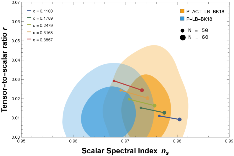
(a) Fixed $s$, varying $c$

(b) Fixed $c$, Varying $s$

Figure 1: Contour plots of the scalar spectral index $n_{s}$ v/s tensor-to-scalar ratio $r$ at pivot scale $k=0.05Mpc^{-1}$. (a) Predictions for $c\in[0.1100,0.3857]$ and fixed $s=0.5110$. (b) Predictions for varying $s\in[0.5005,0.5435]$ and fixed $c=0.2479$. Endpoints of the bars indicate values at N = 50 (small circle) and N = 60 (large circle).The light-shaded region denotes the $95\%$ CL from Planck 2018, and the dark-shaded region shows the $68\%$ CL from the joint Planck 2018 Planck:2018jri, ACT-2025AtacamaCosmologyTelescope:2025blo, and BICEP/Keck 2021 BICEPKeck:2021gln analysis.

(a) Fixed $s$, varying $c$

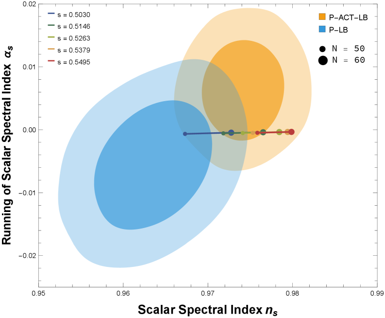
(b) Fixed $c$, Varying $s$

Figure 2: Constraints on the spectral index $n_{s}$ and its running $\alpha_{s}$ pivot scale $k=0.05Mpc^{-1}$ in 68% and 95% confidence levels. The blue contours show results from Planck 2018 data with post lensing+BAO, while the blue contours represent the joint constraints from Planck 2018, ACT DR6, and DESI BAO data. The colored trajectories illustrate theoretical predictions for $N\in[50,60]$ with varying parameter $c\in[0.1100,0.3857]$ at a fixed $s=0.5110$ and $s\in[0.5030,0.5495]$ at a fixed $s=0.2479$, respectively in fig.(a) and fig.(b). The small and big circle mark the $N=50$ and $N=60$ endpoints respectively.

Table 1: Model predictions for varying $c$ (Top Block) and varying $s$ (Bottom Block). Observables are calculated at $N=50$ and $N=60$. Derived parameters are evaluated at $N=60$.

Input		Observables ($N=50$)			Observables ($N=60$)			Derived Parameters ($N=60$)
$c$	$s$	$n_{s}$	$r$	$\alpha_{s}$	$n_{s}$	$r$	$\alpha_{s}$	$\xi$	$\lambda$	$\epsilon$	$\eta$	$H$	$E_{\text{inf}}$
0.1100	0.5110	0.9765	0.0110	-4.69e-04	0.9765	0.0092	-3.26e-04	0.2066	2.85e-15	0.0112	1.51e-02	2.35e-04	0.0720
0.1789	0.5110	0.9730	0.0153	-5.40e-04	0.9730	0.0127	-3.75e-04	0.1603	2.28e-15	0.0112	1.36e-02	2.77e-04	0.0781
0.2479	0.5110	0.9708	0.0197	-5.85e-04	0.9708	0.0164	-4.06e-04	0.1190	1.95e-15	0.0113	1.27e-02	3.14e-04	0.0832
0.3168	0.5110	0.9691	0.0243	-6.17e-04	0.9691	0.0203	-4.29e-04	0.0859	1.75e-15	0.0114	1.20e-02	3.49e-04	0.0878
0.3857	0.5110	0.9678	0.0292	-6.43e-04	0.9678	0.0244	-4.47e-04	0.0609	1.61e-15	0.0115	1.15e-02	3.83e-04	0.0919
0.2479	0.5110	0.9708	0.0197	-5.85e-04	0.9708	0.0164	-4.06e-04	0.1190	1.95e-15	0.0113	1.27e-02	3.14e-04	0.0832
0.2479	0.5206	0.9732	0.0244	-5.36e-04	0.9732	0.0203	-3.72e-04	0.0637	3.21e-15	0.0114	1.37e-02	2.58e-04	0.0754
0.2479	0.5303	0.9746	0.0291	-5.07e-04	0.9746	0.0243	-3.52e-04	0.0472	4.28e-15	0.0115	1.43e-02	2.35e-04	0.0720
0.2479	0.5399	0.9754	0.0339	-4.91e-04	0.9754	0.0283	-3.41e-04	0.0402	5.26e-15	0.0116	1.46e-02	2.23e-04	0.0701
0.2479	0.5495	0.9759	0.0388	-4.83e-04	0.9759	0.0324	-3.35e-04	0.0368	6.19e-15	0.0116	1.48e-02	2.16e-04	0.0690

In Fig. 1, we present the parametric plot of $n_{s}$ versus $r$ for selected values of $c$ and $s$, and for $50\leq N_{*}\leq 60$. The figure shows that the model predictions lie well within the $1\sigma$ confidence regions of the combined data of ACT-2025, Planck-2018 and BICEP/Keck 2021(P-ACT-LB-BK) data. In Fig. 2, we present the marginalized constraints on the scalar spectral index $n_{s}$ and its running $\alpha_{s}$ at the 68% and 95% confidence levels. The blue contours correspond to the constraints obtained from the Planck 2018 data, including post-lensing and baryon acoustic oscillation (BAO) measurements, while the orange contours represent the joint constraints derived from the combined analysis of Planck 2018, ACT DR6, and DESI BAO datasets.

In Fig. 3, we illustrate the behavior of $H(N)$, $\epsilon(N)$, $\lambda(N)$, and $\xi(N)$, evaluated at $N_{*}=60$, for $s\in[0.5030,0.5495]$ and for several representative values of $c\in[0.1100,0.3857]$. The figure shows that the Hubble scale, the inflationary energy scale, and the effective couplings vary smoothly with the torsion–scalar parameters, while the slow-roll parameters $\epsilon$ and $\eta_{\mathcal{R}}$ remain well below unity over the entire inflationary interval. This confirms that the Higgs-like inflationary regime is dynamically stable and that the analytical reconstruction of the model parameters is consistent with sustained slow-roll inflation.And Table 1 summarizes the main results from Fig. 1, Fig. ,Fig. 2 and 3. It lists predicted values of $n_{s}$, $r$, and $\alpha_{s}$ for representative $c$ and $s$ at $N=50$ and $N=60$, with derived quantities at $N=60$. The confidence regions align with current observational bounds and concisely summarize the information from the contour plots.

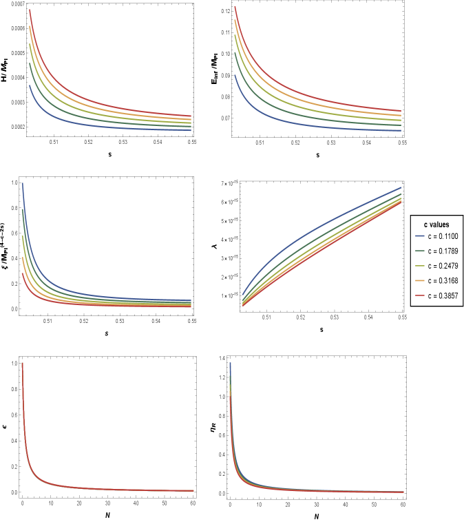
Figure 3: Behavior of the analytically solved background inflationary quantities in our Higgs-like inflation model with $f(T,\phi)$ gravity. The panels display the evolution of the Hubble parameter $H(N_{*})/M_{Pl}$, the inflationary energy scale $E_{\mathrm{inf}}/M_{Pl}$, the non-minimal coupling $\xi(N_{*})/M_{Pl}^{4-c-2s}$, the effective self-coupling $\lambda(N_{*})$, all evaluated at horizon crossing for $N_{*}=60$ for $s\in[0.5030,0.5495]$ and the slow-roll parameters $\epsilon(N)$ & $\eta_{R}(N)$ calculated at $s=0.515$ throught the inflation for number of e-folds N=0 to 60. Each curve corresponds to a distinct choice of $c\in[0.1100,\,0.3875]$, showing how variations in the torsion-Higgs coupling modify the inflationary predictions across the allowed range of the parameter $s$.

We close this section with a comment on the issue of perturbative unitarity. Unitarity has played an important role in the discussion of Higgs inflation in curvature-based gravitational frameworks. In the original Higgs inflation scenario, where the Standard Model Higgs field is nonminimally coupled to the Ricci scalar, the theory exhibits a unitarity cutoff well below the Planck scale for large values of the coupling, raising concerns about the validity of the effective field theory during the inflationary regime Burgess:2009ea; Barbon:2009ya. This issue was later addressed in the so-called “New Higgs inflation” scenario, where a nonminimal derivative coupling between the Higgs field and the Einstein tensor was introduced, leading to a restoration of perturbative unitarity up to the inflationary scale Germani:2010gm; Germani:2011ua. In the present work, however, the situation is fundamentally different. The scalar field $\phi$ driving inflation is not identified with the Standard Model Higgs field, but instead represents a generic Higgs-like inflaton characterized by a quartic symmetry-breaking potential. As a result, the parameters of the potential are not constrained by Standard Model physics, and the theory is not required to remain a low-energy effective extension of particle physics up to the inflationary scale. Consequently, the usual unitarity issues associated with nonminimal Higgs inflation do not arise in our setup. Inflation is instead realized within a scalar-torsion, $f(T,\phi)$ gravitational framework, where the dynamics is controlled by nonminimal couplings between the inflaton and torsion, providing a consistent and predictive effective description throughout the inflationary regime.

V Higgs-like Inflation: Numerical analysis beyond the high-energy approximation

In this section we perform a numerical analysis of the Higgs inflationary scenario by integrating the cosmological equations under the slow-roll approximation, without invoking the dominant-coupling (high-energy) approximation employed in the previous section. This allows us to assess the robustness of the analytical results and to explore the inflationary dynamics in a more general regime.

(a) Fixed $s$ and $\gamma$, varying $c$

(b) Fixed $c$ and $\gamma$, varying $s$

(c) Fixed $c$ and $s$, varying $\gamma$

Figure 4: Constraints in the $n_{s}$–$r$ plane comparing theoretical predictions with current CMB observations at pivot scale $k=0.05Mpc^{-1}$. The shaded contours represent observational confidence regions: the light-shaded region corresponds to the $95\%$ confidence level from Planck 2018, while the dark-shaded region shows the $68\%$ confidence level from the joint Planck 2018 + ACT-2025 + BICEP/Keck 2021 analysisPlanck:2018jriBICEPKeck:2021glnAtacamaCosmologyTelescope:2025blo. (a) Predictions for $s=0.5121$ and $\gamma=10^{-10}$, with the parameter $c$ varied in the range $c\in[0.2150,\,0.4499]$. (b) Predictions for fixed $c=0.3099$ and $\gamma=10^{-10}$, with $s$ varied in the range $s\in[0.5001,\,0.5480]$. (c) Predictions for fixed $c=0.3099$ and $s=0.5121$, with $\gamma$ varied over the indicated values. In all panels, the endpoints of each theoretical trajectory correspond to the number of e-folds $N=50$ (small markers) and $N=60$ (large markers).

For convenience, we introduce the auxiliary variable (setting $M_{Pl}=1$)

$$Y(N)=2\xi(2s-1)\,\phi(N)^{c}\,T(N)^{\,s-1},$$ (106)

such that the effective gravitational coupling can be written as

$$\mathcal{G}_{eff}(N)=\frac{\mathcal{G}}{1+Y(N)}.$$ (107)

In the limit $Y\gg 1$, the theory enters the dominant-coupling regime discussed in the previous section.

This definition allows us to rewrite the background equations in a compact form. Assuming the Higgs potential (90) in the large-field regime $\phi^{2}\gg\nu^{2}$—or, more generally, a monomial potential of the form $V(\phi)=\lambda\phi^{d}/d$ with $d=4$—together with the coupling function (91), the first Friedmann equation in the slow-roll approximation can be expressed as

$$\left(2(2s-1)\right)^{\frac{1}{1-s}}(Y+1)\,Y^{\frac{1}{s-1}}\,\phi^{\frac{c}{1-s}}-2\gamma\,\phi^{d}=0,$$ (108)

where we have defined the parameter

$$\gamma\equiv\frac{\lambda}{d\>\xi^{\frac{1}{1-s}}}.$$ (109)

Equation (108) can be solved algebraically for the scalar field as a function of $Y(N)$, yielding

$$\phi(N)=\left[\frac{2\gamma\,Y(N)^{\frac{1}{1-s}}}{\left(2(2s-1)\right)^{\frac{1}{1-s}}\left(Y(N)+1\right)}\right]^{\frac{1}{\frac{c}{1-s}-d}}.$$ (110)

On the other hand, the equation of motion for the scalar field, written in terms of the number of e-folds and evaluated under the slow-roll approximation, takes the form

$$\frac{d\phi}{dN}=\frac{\gamma d\left(2(2s-1)\right)^{\frac{s}{s-1}}Y(N)^{\frac{1}{1-s}}\phi(N)^{\frac{c}{s-1}+d}+c\,Y(N)}{(2s-1)\,\phi(N)}.$$ (111)

Taking the derivative of (108) and using (111) and (110), we obtain

$$\frac{dY}{dN}=\frac{\mathcal{A}Y^{1-\frac{2}{c+d(s-1)}}(Y+1)^{\frac{c+(d-2)(s-1)}{c+d(s-1)}}\left(c2^{\frac{s}{s-1}}Y+d(4s-2)^{\frac{s}{s-1}}(2s-1)^{\frac{1}{1-s}}(Y+1)\right)}{sY+1},$$ (112)

where

$$\mathcal{A}=2^{-\frac{s(c+(d-2)(s-1))}{(s-1)(c+d(s-1))}}\gamma^{\frac{2(s-1)}{c+d(s-1)}}(c+d(s-1))(2s-1)^{\frac{2}{c+d(s-1)}-1}.$$ (113)

is a constant. Equations (110) and (112) form a closed system that can be integrated numerically to determine the full inflationary evolution without relying on the dominant-coupling (high-energy) approximation.

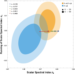
(a) Fixed $s$ and $\gamma$, varying $c$

(b) Fixed $c$ and $\gamma$, varying $s$

(c) Fixed $c$ and $s$, varying $\gamma$

Figure 5: Constraints in the $n_{s}$–$\alpha_{s}$ plane comparing theoretical predictions with current CMB observations at pivot scale $k=0.05Mpc^{-1}$. The shaded contours denote observational confidence regions: the light-shaded region corresponds to the $95\%$ confidence level from Planck 2018, while the dark-shaded region represents the $68\%$ confidence level from the joint Planck 2018 + ACT-2025 + BICEP/Keck 2021 analysis. (a) Predictions for $s=0.5121$ and $\gamma=10^{-10}$, with the parameter $c$ varied in the range $c\in[0.2150,\,0.4499]$. (b) Predictions for fixed $c=0.3099$ and $\gamma=10^{-10}$, with $s$ varied in the range $s\in[0.5001,\,0.5480]$. (c) Predictions for fixed $c=0.3099$ and $s=0.5121$, with $\gamma$ varied over the indicated values. In all panels, the endpoints of each theoretical trajectory correspond to the number of e-folds $N=50$ (small markers) and $N=60$ (large markers).

In Fig. 7, we illustrate the behavior of $H(N)$, $\epsilon(N)$, $\lambda(N)$, and $\xi(N)$, outside the high energy regime and evaluated at $N_{*}=60$, for $s\in[0.5001,0.5480]$ and for several representative values of $c\in[0.2150,0.4499]$. The figure shows that the Hubble scale, the inflationary energy scale, and the effective couplings vary smoothly with the torsion–scalar parameters, while the slow-roll parameters $\epsilon$ and $\eta_{\mathcal{R}}$ remain well below unity over the entire inflationary interval. This confirms that our model remains dynamically stable even outside the high-energy regime. Furthermore, Fig. 6 illustrates the role of the coupling function $Y(\phi)$ (or $\mathcal{G}_{eff}(\phi)$) across different energy scales. In particular, smaller values of the parameter $\gamma$ drive the system toward the high-energy approximation, characterized by large values of both $Y(\phi)$ and the inflaton field $\phi$, reaching trans-Planckian field values. In this regime, the coupling term dominates the dynamics, placing the model firmly in the dominant-coupling regime and providing a smooth connection with the results obtained in the previous section. Conversely, increasing $\gamma$ shifts the dynamics toward lower values of $Y(\phi)$ and $\phi$. However, this regime is strongly constrained by observational data, since larger values of $\gamma$ lead to an enhanced tensor-to-scalar ratio $r$, pushing the predictions outside the $2\sigma$ confidence region.

The scalar power spectrum is given by

$$\mathcal{P}_{s}(N_{*})=\frac{2^{-\frac{3}{s-1}-5}(2s-1)^{-\frac{3}{s-1}}\xi^{\frac{1}{1-s}}\phi_{*}^{2-\frac{c}{s-1}}Y_{*}^{\frac{3}{s-1}}}{3\pi^{2}\left(d\gamma\phi^{\frac{c}{s-1}+d}+c(4s-2)^{\frac{s}{1-s}}Y_{*}^{\frac{s}{s-1}}\right)^{2}},$$ (114)

where $\phi(N_{*})\equiv\phi_{*}$, $Y(N_{*})\equiv Y_{*}$.

Thus, solving for $\xi$ we get

$$\xi(N_{*})=\frac{2^{2-5s}3^{1-s}\pi^{2-2s}Y_{*}^{3}\mathcal{P}_{s}^{1-s}\phi_{*}^{-c+2s-2}\left(d\gamma\phi_{*}^{\frac{c}{s-1}+d}+c(4s-2)^{\frac{s}{1-s}}Y_{*}^{\frac{s}{s-1}}\right)^{2-2s}}{(2s-1)^{3}},$$ (115)

and

$$\lambda(N_{*})=\gamma d\>\xi(N_{*})^{\frac{1}{1-s}}.$$ (116)

The spectral index takes the form

$$n_{s}(N_{*})=1+\frac{2(c-1)cY_{*}}{(2s-1)\phi_{*}^{2}}+(d-1)d\gamma 2^{\frac{1}{s-1}+2}(2s-1)^{\frac{1}{s-1}}Y_{*}^{\frac{1}{1-s}}\phi_{*}^{\frac{c}{s-1}+d-2}-$$

$$\frac{cd\gamma 2^{\frac{1}{1-s}+2}(2s-1)^{-\frac{s}{s-1}}(4s-2)^{\frac{2}{s-1}}Y_{*}^{\frac{s-2}{s-1}}(s(3s-1)Y_{*}+s(7-2s)-3)\phi_{*}^{\frac{c}{s-1}+d-2}}{(sY_{*}+1)(sY_{*}+2s-1)}+$$

$$\frac{c^{2}Y_{*}\left[Y_{*}\left(3+s\left(-4s^{2}+2s-5\right)-s\left(2s^{2}+s-1\right)Y_{*}\right)+2s(1-2s)\right]}{(s-1)(2s-1)\phi_{*}^{2}(sY_{*}+1)(sY+2s-1)}-$$

$$\frac{2d^{2}\gamma^{2}(2s-1)^{\frac{1}{s-1}}Y_{*}^{-\frac{2}{s-1}}\left[s\left(2^{\frac{1}{s-1}+3}s-2^{\frac{s}{s-1}}\right)(4s-2)^{\frac{1}{s-1}}Y_{*}+3\ 2^{\frac{s+1}{s-1}}(2s-1)^{\frac{s}{s-1}}\right]\phi_{*}^{2\left(\frac{c}{s-1}+d-1\right)}}{(sY_{*}+1)(sY_{*}+2s-1)},$$ (117)

and its running is given by

$$\alpha_{s}(N_{*})=\;\frac{1}{(s-1)(2s-1)\,(1+sY_{*})^{3}\,(2s-1+sY_{*})^{2}\,\phi_{*}^{3}}\sum_{i=1}^{11}\mathcal{F}_{i}(\phi_{*},Y_{*}).$$

where $\mathcal{F}_{i}(\phi_{*},Y_{*})$ functions are defined in appendix B.

On the other hand, the tensor-to-scalar ratio reads

$$r(N_{*})=\frac{2^{\frac{2}{s-1}+5}(2s-1)^{\frac{s+1}{s-1}}Y_{*}^{-\frac{2}{s-1}}\left(d\gamma\phi_{*}^{\frac{c}{s-1}+d}+c(4s-2)^{\frac{s}{1-s}}Y_{*}^{\frac{s}{s-1}}\right)^{2}}{\phi_{*}^{2}(s(Y_{*}+2)-1)}.$$ (118)

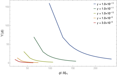
Figure 6: Parametric plots showing the evolution of the auxiliary variable $Y(\phi)$ as a function of the scalar field $\phi$ for different values of the parameter $\gamma$, illustrating the sensitivity of the field dynamics to the coupling strength. The other model parameters are fixed at $s=0.511$, $c=0.3119$. The trajectories represent the evolution over $N=60$ e-folds of inflation.

In Fig. 4, we present the parametric trajectories of the scalar spectral index $n_{s}$ versus the tensor-to-scalar ratio $r$.These theoretical predictions are obtained by fully integrating the slow-roll equations without assuming the dominant-coupling (high-energy) approximation. We explore the parameter space by varying $c\in[0.2150,0.4499]$ and $s\in[0.5001,0.5480]$, alongside the coupling parameter $\gamma$, for the number of e-folds $50\leq N_{*}\leq 60$. The results demonstrate that, even outside the high-energy limit, the model predictions remain robust and lie well within the $1\sigma$ and $2\sigma$ confidence regions of the combined dataset from Planck 2018, ACT DR6 (ACT-2025), and BICEP/Keck 2021.

In, Fig. 5 presents the marginalized constraints in the $n_{s}-\alpha_{s}$ plane. The theoretical predictions for the running of the scalar spectral index are consistent with the $68\%$ and $95\%$ confidence intervals derived from the joint Planck, ACT, and DESI analysis. Table 2 summarizes these findings, listing the specific values for $n_{s}$, $r$, and $\alpha_{s}$, along with the derived model parameters at $N=60$. The table confirms that the numerical results align with current observational bounds. Furthermore, Fig. 6 depicts the behavior of the auxiliary variable $Y(\phi)$. The large values of $Y(\phi)$ observed at high energies (large field values) confirm that the scalar-torsion coupling dominates early in the inflationary phase, thereby validating the dominant-coupling approximation used in our analytical study, while the numerical solution captures the exact dynamics as this dominance relaxes.

Finally, In Fig. 7 illustrates the evolution of the key background quantities—the Hubble parameter $H(N_{*})$, the inflationary energy scale $E_{\text{inf}}$, the non-minimal coupling $\xi(N_{*})$, and the effective self-coupling $\lambda(N_{*})$—evaluated at $N_{*}=60$. It also displays the slow-roll parameters $\epsilon$ and $\eta_{\mathcal{R}}$ throughout the inflationary epoch. The smooth variation of the background fields and the fact that the slow-roll parameters remain much smaller than unity ($\epsilon,|\eta_{\mathcal{R}}|\ll 1$) confirm the dynamical stability of the inflationary solution across the explored parameter range.

Table 2: Numerical predictions for inflationary observables and derived model parameters. The table is divided into three blocks corresponding to variations in $c$ (top), $s$ (middle), and $\gamma$ (bottom). Observables are reported for $N=50$ and $N=60$ e-folds, while derived parameters are evaluated at $N=60$.

Input			Observables ($N=50$)			Observables ($N=60$)			Derived Parameters ($N=60$)
$c$	$s$	$\gamma$	$n_{s}$	$r$	$\alpha_{s}$	$n_{s}$	$r$	$\alpha_{s}$	$\xi$	$\lambda$	$\epsilon$	$\eta$	$H$	$E_{\text{inf}}$
0.2150	0.5121	$10^{-10}$	0.9767	0.0237	-4.88e-04	0.9767	0.0203	-3.37e-04	0.0041	1.27e-15	0.0103	0.1516	9.29e-05	0.0453
0.2737	0.5121	$10^{-10}$	0.9744	0.0274	-5.29e-04	0.9744	0.0234	-3.66e-04	0.0038	1.08e-15	0.0104	0.1350	1.05e-04	0.0480
0.3325	0.5121	$10^{-10}$	0.9726	0.0312	-5.62e-04	0.9726	0.0265	-3.90e-04	0.0035	9.25e-16	0.0105	0.1228	1.18e-04	0.0510
0.3912	0.5121	$10^{-10}$	0.9710	0.0351	-5.89e-04	0.9710	0.0297	-4.09e-04	0.0033	8.09e-16	0.0106	0.1135	1.34e-04	0.0543
0.4499	0.5121	$10^{-10}$	0.9696	0.0391	-6.14e-04	0.9696	0.0330	-4.26e-04	0.0031	7.18e-16	0.0107	0.1064	1.52e-04	0.0579
0.3099	0.5110	$10^{-10}$	0.9731	0.0294	-5.52e-04	0.9731	0.0250	-3.83e-04	0.0035	9.53e-16	0.0104	0.1226	1.12e-04	0.0496
0.3099	0.5203	$10^{-10}$	0.9740	0.0329	-5.32e-04	0.9740	0.0279	-3.69e-04	0.0043	1.17e-15	0.0108	0.1553	1.20e-04	0.0514
0.3099	0.5295	$10^{-10}$	0.9746	0.0371	-5.16e-04	0.9746	0.0313	-3.59e-04	0.0052	1.39e-15	0.0111	0.1785	1.28e-04	0.0531
0.3099	0.5388	$10^{-10}$	0.9749	0.0415	-5.06e-04	0.9749	0.0350	-3.52e-04	0.0061	1.61e-15	0.0113	0.1953	1.35e-04	0.0546
0.3099	0.5480	$10^{-10}$	0.9750	0.0461	-5.02e-04	0.9750	0.0389	-3.49e-04	0.0072	1.83e-15	0.0115	0.2076	1.42e-04	0.0560
0.3099	0.5121	$10^{-12}$	0.9710	0.0254	-5.83e-04	0.9710	0.0213	-4.06e-04	0.0263	5.77e-16	0.0110	0.1216	2.24e-04	0.0703
0.3099	0.5121	$10^{-11}$	0.9719	0.0269	-5.71e-04	0.9719	0.0227	-3.97e-04	0.0094	7.03e-16	0.0108	0.1227	1.56e-04	0.0586
0.3099	0.5121	$10^{-10}$	0.9732	0.0297	-5.50e-04	0.9732	0.0253	-3.81e-04	0.0036	9.78e-16	0.0104	0.1271	1.13e-04	0.0498
0.3099	0.5121	$10^{-9}$	0.9749	0.0350	-5.21e-04	0.9749	0.0300	-3.60e-04	0.0015	1.57e-15	0.0103	0.1383	8.57e-05	0.0435
0.3099	0.5121	$3\times 10^{-9}$	0.9757	0.0388	-5.05e-04	0.9757	0.0335	-3.49e-04	0.0010	2.05e-15	0.0103	0.1470	7.67e-05	0.0411

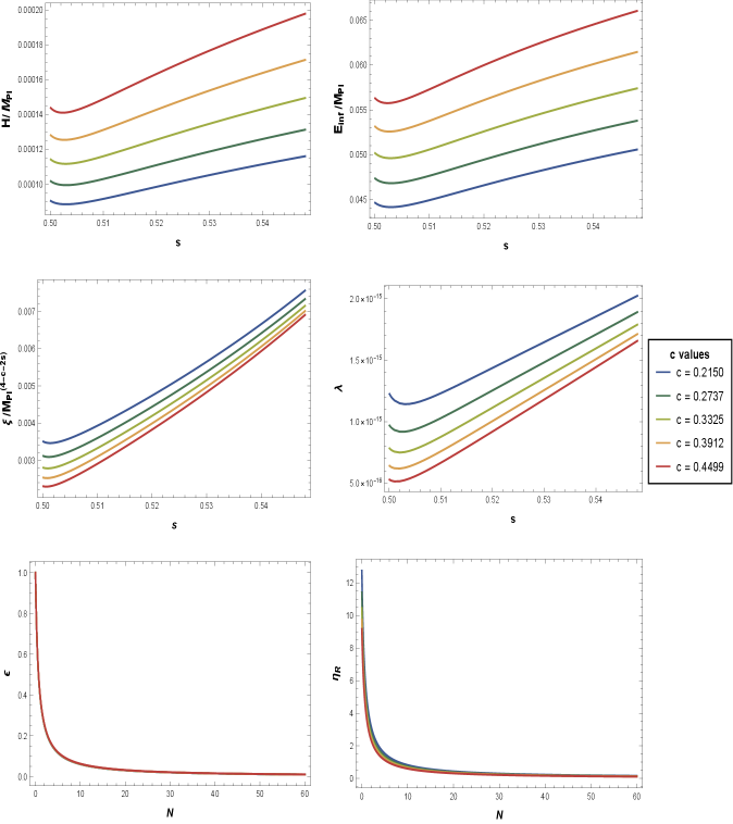
Figure 7: Behavior of the background inflationary quantities in our Higgs-like inflation model with $f(T,\phi)$ gravity calculated with full numerical integration. the Hubble parameter $H(N_{*})/M_{Pl}$, the inflationary energy scale $E_{\mathrm{inf}}/M_{Pl}$, the non-minimal coupling $\xi(N_{*})/M_{Pl}^{4-c-2s}$, the effective self-coupling $\lambda(N_{*})$, all evaluated at horizon crossing for $N_{*}=60$ for $s\in[0.5001,0.5480]$ and the slow-roll parameters $\epsilon(N)$ & $\eta_{R}(N)$ calculated at $s=0.5121$ throught the inflation $N=60-0$. $\gamma=10^{-10}$ is fixed in all of these plots to be away from the high energy regieme as done in section III.2. Each curve corresponds to a distinct choice of $c\in[0.2150,0.4499]$, showing how variations in the torsion-Higgs coupling modify the inflationary predictions across the allowed range of the parameter $s$.

VI Conclusions

In this work we have investigated Higgs-driven inflation within the framework of scalar-torsion gravity, focusing on the general class of $f(T,\phi)$ theories. The motivation for this study is twofold. On one hand, Higgs inflation provides an attractive bridge between high-energy physics and the early Universe, but its viability is increasingly scrutinized by the steadily improving precision of cosmological observations. On the other hand, torsion-based extensions of gravity constitute a conceptually distinct alternative to curvature-based theories, giving rise to genuinely new gravitational interactions and cosmological dynamics. In view of the latest CMB and large-scale-structure constraints from Planck, ACT, DESI, and BICEP/Keck, it is therefore timely to reassess Higgs-like inflationary scenarios within a scalar-torsion gravitational setting.

We first developed the general theoretical framework of $f(T,\phi)$ gravity at the background and perturbative levels, emphasizing the distinctive role played by torsion-induced interactions and the associated departure from local Lorentz invariance. Within the slow-roll approximation, we derived the background equations, the second-order action for scalar and tensor perturbations, and the corresponding inflationary observables. A central element of our analysis is the dominant-coupling (high-energy) regime, in which the scalar-torsion interaction governs the inflationary dynamics. In this limit, we obtained closed-form analytical expressions for the scalar spectral index $n_{s}$ and the tensor-to-scalar ratio $r$ as functions of the number of e-folds. These results reveal characteristic deviations from standard single-field inflation and modified consistency relations that encode torsion effects in a transparent and testable manner.

Specializing to Higgs-like inflation, we imposed a quartic symmetry-breaking potential together with a power-law scalar-torsion coupling and we derived explicit analytical predictions for the inflationary observables. We showed that, in the dominant-coupling regime, the model naturally yields values of $n_{s}$ and $r$ fully consistent with current observational bounds, including the latest joint constraints from Planck, ACT, DESI, and BICEP/Keck. Notably, the $f(T,\phi)$ framework accommodates the upward shift in the preferred value of $n_{s}$, which places increasing pressure on several plateau-type inflationary models. We further derived parametric relations between $n_{s}$ and $r$, as well as explicit expressions for the effective self-coupling and nonminimal coupling parameters, clarifying how torsion modifies both the inflationary dynamics and the effective gravitational interaction.

To assess the robustness of these analytical results, we performed a detailed numerical analysis beyond the dominant-coupling approximation, integrating the slow-roll equations without invoking additional simplifying assumptions. This allowed us to follow the full inflationary evolution and to verify that the analytical predictions remain accurate across a wide region of parameter space. The numerical solutions confirm that Higgs-like inflation in $f(T,\phi)$ gravity is stable, predictive, and compatible with current data, while also exhibiting distinctive signatures in the tensor sector and in the scale dependence of the scalar spectrum that are absent in curvature-based realizations. Additionally, as we discussed, the scenario is free from any unitaity issues, such as those that arise in Higgs inflation in curvature-based theories.

In conclusion, our results demonstrate that $f(T,\phi)$ gravity provides a viable and theoretically well-motivated framework in which Higgs-like inflation can be reconciled with precision cosmology. The characteristic inflationary signatures induced by scalar-torsion couplings offer concrete targets for upcoming CMB polarization experiments and next-generation large-scale-structure surveys. Extensions of the present analysis to include reheating, primordial black-hole formation, or non-Gaussianities, represent promising directions and will be studied in future works.

Appendix A The running of the scalar spectral index $\alpha_{s}$

In the scenario at hand, the running of the scalar spectral index is given by

$$\alpha_{s}\equiv\frac{dn_{s}}{d\ln k}=\frac{\sqrt{6}}{T^{7/2}}\left[\Theta_{1}+4(\Theta_{2}+\Theta_{3})+\Theta_{4}\right],$$ (119)

where $\Theta_{1}$, $\Theta_{2}$, $\Theta_{3}$ and $\Theta_{4}$ are given by

$$\Theta_{1}\equiv{} \frac{4\,(GF_{,\phi}+V_{,\phi})\big(F_{,\phi}(G-2TG_{,T})+V_{,\phi}\big)}{M_{Pl}^{2}+2F(G_{,T}+2TG_{,TT})}$$

$$\times\Bigg[-2\dot{T}+\frac{T\big(F_{,\phi}G_{,T}\dot{T}+\dot{\phi}(GF_{,\phi\phi}+V_{,\phi\phi})\big)}{GF_{,\phi}+V_{,\phi}}$$

$$\qquad+\frac{T\big(-F_{,\phi}\dot{T}(G_{,T}+2TG_{,TT})+\dot{\phi}\big((G-2TG_{,T})F_{,\phi\phi}+V_{,\phi\phi}\big)\big)}{F_{,\phi}(G-2TG_{,T})+V_{,\phi}}$$

$$\qquad-\frac{2T\big(F_{,\phi}\dot{\phi}(G_{,T}+2TG_{,TT})+F\dot{T}(3G_{,TT}+2TG_{,TTT})\big)}{M_{Pl}^{2}+2F(G_{,T}+2TG_{,TT})}\Bigg],$$

$$\Theta_{2}\equiv{} -\frac{2T^{2}F_{,\phi}^{2}G_{,T}\dot{T}}{F}+\frac{4\dot{T}\,(GF_{,\phi}+V_{,\phi})^{2}}{M_{Pl}^{2}+2FG_{,T}}+\frac{T\,F_{,\phi}^{2}G_{,T}^{2}\dot{T}}{F\,G_{,TT}}+\frac{T^{2}F_{,\phi}^{3}G_{,T}^{2}\dot{\phi}}{F^{2}G_{,TT}}-\frac{2T^{2}F_{,\phi}G_{,T}^{2}\dot{\phi}\,F_{,\phi\phi}}{F\,G_{,TT}}$$

$$\quad+\frac{4T\,(GF_{,\phi}+V_{,\phi})^{2}\big(F_{,\phi}G_{,T}\dot{\phi}+F\dot{T}\,G_{,TT}\big)}{(M_{Pl}^{2}+2FG_{,T})^{2}}$$

$$\quad-\frac{4\dot{T}\big(F_{,\phi}(G-2TG_{,T})+V_{,\phi}\big)\big(F_{,\phi}(G-TG_{,T})+V_{,\phi}\big)}{M_{Pl}^{2}+2F(G_{,T}+2TG_{,TT})}$$

$$\quad+\frac{2T\big(F_{,\phi}(G-2TG_{,T})+V_{,\phi}\big)\Big((G-TG_{,T})\dot{\phi}\,F_{,\phi\phi}-TF_{,\phi}\dot{T}\,G_{,TT}+\dot{\phi}\,V_{,\phi\phi}\Big)}{M_{Pl}^{2}+2F(G_{,T}+2TG_{,TT})},$$

$$\Theta_{3}\equiv{} -\frac{4T\,(GF_{,\phi}+V_{,\phi})\big(F_{,\phi}G_{,T}\dot{T}+\dot{\phi}\,(GF_{,\phi\phi}+V_{,\phi\phi})\big)}{M_{Pl}^{2}+2FG_{,T}}$$

$$\quad+\frac{2T\big(F_{,\phi}(G-TG_{,T})+V_{,\phi}\big)\Big(-F_{,\phi}\dot{T}\,(G_{,T}+2TG_{,TT})+\dot{\phi}\big((G-2TG_{,T})F_{,\phi\phi}+V_{,\phi\phi}\big)\Big)}{M_{Pl}^{2}+2F(G_{,T}+2TG_{,TT})}$$

$$\quad+\frac{T^{2}F_{,\phi}^{2}G_{,T}^{2}\dot{T}\,G_{,TTT}}{F\,G_{,TT}^{2}}$$

$$\quad-\frac{2T\big(F_{,\phi}(G-2TG_{,T})+V_{,\phi}\big)\big(F_{,\phi}(G-TG_{,T})+V_{,\phi}\big)\Big(2F_{,\phi}\dot{\phi}\,(G_{,T}+2TG_{,TT})+2F\dot{T}\,(3G_{,TT}+2TG_{,TTT})\Big)}{\big(M_{Pl}^{2}+2F(G_{,T}+2TG_{,TT})\big)^{2}},$$

$$\!\!\!\!\!\!\!\!\!\!\!\!\!\!\!\!\!\!\!\!\!\!\!\!\!\!\!\!\!\!\!\!\!\!\!\!\!\!\!\!\!\!\!\!\!\!\Theta_{4}\equiv{} \frac{1}{M_{Pl}^{2}+2F(G_{,T}+2TG_{,TT})}\;\mathcal{A}\,\mathcal{B},$$

with

$$\mathcal{A}\equiv{} 8G^{2}F_{,\phi}^{2}+8\big(TF_{,\phi}G_{,T}-V_{,\phi}\big)\big(2TF_{,\phi}G_{,T}-V_{,\phi}\big)$$

$$\quad-4G\Big(-4F_{,\phi}V_{,\phi}+T\big(6F_{,\phi}^{2}G_{,T}+(M_{Pl}^{2}+2FG_{,T})F_{,\phi\phi}\big)+4FT^{2}F_{,\phi\phi}G_{,TT}\Big)$$

$$\quad-4T\big(M_{Pl}^{2}+2F(G_{,T}+2TG_{,TT})\big)V_{,\phi\phi},$$

$$\mathcal{B}\equiv{} -2\dot{T}-\frac{2T\big(F_{,\phi}\dot{\phi}(G_{,T}+2TG_{,TT})+F\dot{T}(3G_{,TT}+2TG_{,TTT})\big)}{M_{Pl}^{2}+2F(G_{,T}+2TG_{,TT})},$$

$$\quad+\frac{T}{\mathcal{D}}\Big(2F_{,\phi}G_{,T}\dot{T}\,V_{,\phi}-4G^{2}F_{,\phi}\dot{\phi}\,F_{,\phi\phi}+\big((M_{Pl}^{2}+2FG_{,T})\dot{T}-4V_{,\phi}\dot{\phi}\big)V_{,\phi\phi}$$

$$\qquad+G\Big(2F_{,\phi}^{2}\dot{T}(G_{,T}+3TG_{,TT})+2F_{,\phi}\dot{\phi}\big(TF_{,\phi\phi}(7G_{,T}+2TG_{,TT})-2V_{,\phi\phi}\big)$$

$$\qquad\qquad+\dot{\phi}\big(-4V_{,\phi}F_{,\phi\phi}+T\big(M_{Pl}^{2}+2F(G_{,T}+2TG_{,TT})\big)F_{,\phi\phi\phi}\big)$$

$$\qquad\qquad+\dot{T}\,F_{,\phi\phi}\big(M_{Pl}^{2}+2F(G_{,T}+5TG_{,TT}+2T^{2}G_{,TTT})\big)\Big)$$

$$\qquad+T\Big(-2F_{,\phi}^{2}G_{,T}^{2}\dot{T}+2FG_{,T}^{2}\dot{T}\,F_{,\phi\phi}+0F\dot{T}\,G_{,TT}V_{,\phi\phi}$$

$$\qquad\qquad+F_{,\phi}\big(6\dot{T}\,V_{,\phi}G_{,TT}+8G_{,T}\dot{\phi}\,V_{,\phi\phi}\big)+M_{Pl}^{2}\dot{\phi}\,V_{,\phi\phi\phi}$$

$$\qquad\qquad+G_{,T}\big((M_{Pl}^{2}\dot{T}+6V_{,\phi}\dot{\phi})F_{,\phi\phi}+2F\dot{\phi}\,V_{,\phi\phi\phi}\big)\Big)$$

$$\qquad+4T^{2}\Big(-2F_{,\phi}^{2}G_{,T}\dot{T}\,G_{,TT}+F_{,\phi}\dot{\phi}\big(-2G_{,T}^{2}F_{,\phi\phi}+G_{,TT}V_{,\phi\phi}\big)$$

$$\qquad\qquad+F\big(\dot{T}(G_{,T}F_{,\phi\phi}G_{,TT}+V_{,\phi\phi}G_{,TTT})+\dot{\phi}\,G_{,TT}V_{,\phi\phi\phi}\big)\Big)\Big).$$

$$\mathcal{D}\equiv{} -2\,G^{2}F_{,\phi}^{2}-2\big(TF_{,\phi}G_{,T}-V_{,\phi}\big)\big(2TF_{,\phi}G_{,T}-V_{,\phi}\big)$$

$$\quad+G\Big(-4F_{,\phi}V_{,\phi}+T\big(6F_{,\phi}^{2}G_{,T}+(M_{Pl}^{2}+2FG_{,T})F_{,\phi\phi}\big)+4FT^{2}F_{,\phi\phi}G_{,TT}\Big)$$

$$\quad+T\big(M_{Pl}^{2}+2F(G_{,T}+2TG_{,TT})\big)V_{,\phi\phi}.$$

Appendix B The running of the scalar spectral index $\alpha_{s}(\phi_{*},Y_{*})$ beyond the high-energy approximation

For the case beyond the high-energy approximation, the running of the scalar spectral index is given by

$$\alpha_{s}(\phi_{*},Y_{*})\equiv\;\frac{1}{(-1+s)(-1+2s)\,(1+sY_{*})^{3}\,(-1+2s+sY_{*})^{2}\,\phi_{*}^{3}}\sum_{i=1}^{11}\mathcal{F}_{i}(\phi_{*},Y_{*}),$$

where $\mathcal{F}_{i}(\phi_{*},Y_{*})$ functions are given by

$$\mathcal{F}_{1}(\phi_{*},Y_{*})\equiv 2^{\frac{c(-2+s)+(-1+s)\bigl(d(-2+s)+s\bigr)}{\bigl(c+d(-1+s)\bigr)(-1+s)}}\,(c-1)c\,\gamma^{\frac{-1+s}{c+d(-1+s)}}\,(-1+s)\,(-1+2s)^{-1+\frac{1}{c+d(-1+s)}}$$

$$\times Y_{*}^{\,1-\frac{2}{-1+s}+\frac{1}{-c+d-ds}}\,(1+Y_{*})^{-\frac{c+(1+d)(-1+s)}{c+d(-1+s)}}\,(1+sY_{*})^{3}\,(-1+2s+sY_{*})^{2}$$

$$\times\Bigl(Y_{*}^{\frac{1}{-1+s}}+Y_{*}^{\frac{s}{-1+s}}\Bigr)\,\mathcal{K}_{1}(Y_{*}),$$

$$\mathcal{F}_{2}(\phi_{*},Y_{*})\equiv -2^{-\frac{c+(d-s)(-1+s)}{\bigl(c+d(-1+s)\bigr)(-1+s)}}\,\gamma^{\frac{-1+s}{c+d(-1+s)}}\,(-1+2s)^{-1+\frac{1}{c+d(-1+s)}}\,Y_{*}^{\,1-\frac{2}{-1+s}+\frac{1}{-c+d-ds}}$$

$$\times(1+Y_{*})^{-\frac{c+(1+d)(-1+s)}{c+d(-1+s)}}\,(-1+2s+sY_{*})\,\bigl(c+csY_{*}\bigr)^{2}$$

$$\times\Bigl(2s(-1+2s)+(-3+5s-2s^{2}+4s^{3})Y_{*}+s(-1+s+2s^{2})Y_{*}^{2}\Bigr)\Bigl(Y_{*}^{\frac{1}{-1+s}}+Y_{*}^{\frac{s}{-1+s}}\Bigr)\,\mathcal{K}_{1}(Y_{*}),$$

$$\mathcal{F}_{3}(\phi_{*},Y_{*})\equiv 2^{-\frac{s\bigl(c+(-2+d)(-1+s)\bigr)}{\bigl(c+d(-1+s)\bigr)(-1+s)}}\,c^{2}\,\gamma^{\frac{2(-1+s)}{c+d(-1+s)}}\,\bigl(c+d(-1+s)\bigr)\,(-1+2s)^{-1+\frac{2}{c+d(-1+s)}}$$

$$\times Y_{*}^{\,2-\frac{2}{c+d(-1+s)}-\frac{2}{-1+s}}\,(1+Y_{*})^{\frac{2-2s}{c+d(-1+s)}}\,(1+sY_{*})\,(-1+2s+sY_{*})$$

$$\times\Bigl(-3+5s-2s^{2}+4s^{3}+2s(-1+s+2s^{2})Y_{*}\Bigr)\Bigl(Y_{*}^{\frac{1}{-1+s}}+Y_{*}^{\frac{s}{-1+s}}\Bigr)\,\mathcal{K}_{1}(Y_{*})\;\phi_{*},$$

$$\mathcal{F}_{4}(\phi_{*},Y_{*})\equiv 2^{\,1-\frac{s\bigl(c+(-2+d)(-1+s)\bigr)}{\bigl(c+d(-1+s)\bigr)(-1+s)}}\,(1-c)c\,\gamma^{\frac{2(-1+s)}{c+d(-1+s)}}\,\bigl(c+d(-1+s)\bigr)\,(1-s)\,(-1+2s)^{-1+\frac{2}{c+d(-1+s)}}$$

$$\times Y_{*}^{\,1-\frac{2}{c+d(-1+s)}-\frac{2}{-1+s}}\,(1+Y_{*})^{\frac{2-2s}{c+d(-1+s)}}\,(1+sY_{*})^{2}\,(-1+2s+sY_{*})^{2}$$

$$\times\Bigl(Y_{*}^{\frac{1}{-1+s}}+Y_{*}^{\frac{s}{-1+s}}\Bigr)\,\mathcal{K}_{1}(Y_{*})\;\phi_{*},$$

$$\mathcal{F}_{5}(\phi_{*},Y_{*})\equiv -2^{-\frac{s\bigl(c+(-2+d)(-1+s)\bigr)}{\bigl(c+d(-1+s)\bigr)(-1+s)}}\,c^{2}\,\gamma^{\frac{2(-1+s)}{c+d(-1+s)}}\,\bigl(c+d(-1+s)\bigr)\,s\,(-1+2s)^{-1+\frac{2}{c+d(-1+s)}}$$

$$\times Y_{*}^{\,2-\frac{2}{c+d(-1+s)}-\frac{2}{-1+s}}\,(1+Y_{*})^{\frac{2-2s}{c+d(-1+s)}}\,(1-2s-sY_{*})$$

$$\times\Bigl(Y_{*}^{\frac{1}{-1+s}}+Y_{*}^{\frac{s}{-1+s}}\Bigr)\,\mathcal{K}_{1}(Y_{*})$$

$$\times\Bigl(2(1-2s)s+Y_{*}\bigl(3+s(-5+2s-4s^{2})-s(-1+s+2s^{2})Y_{*}\bigr)\Bigr)\,\phi_{*},$$

$$\mathcal{F}_{6}(\phi_{*},Y_{*})\equiv 2^{-\frac{s\bigl(c+(-2+d)(-1+s)\bigr)}{\bigl(c+d(-1+s)\bigr)(-1+s)}}\,c^{2}\,\gamma^{\frac{2(-1+s)}{c+d(-1+s)}}\,\bigl(c+d(-1+s)\bigr)\,s\,(-1+2s)^{-1+\frac{2}{c+d(-1+s)}}$$

$$\times Y_{*}^{\,2-\frac{2}{c+d(-1+s)}-\frac{2}{-1+s}}\,(1+Y_{*})^{\frac{2-2s}{c+d(-1+s)}}\,(1+sY_{*})$$

$$\times\Bigl(Y_{*}^{\frac{1}{-1+s}}+Y_{*}^{\frac{s}{-1+s}}\Bigr)\,\mathcal{K}_{1}(Y_{*})$$

$$\times\Bigl(2(1-2s)s+Y_{*}\bigl(3+s(-5+2s-4s^{2})-s(-1+s+2s^{2})Y_{*}\bigr)\Bigr)\,\phi_{*},$$

$$\mathcal{F}_{7}(\phi_{*},Y_{*})\equiv 2^{-\frac{s\bigl(c+(-2+d)(-1+s)\bigr)}{\bigl(c+d(-1+s)\bigr)(-1+s)}}\,c^{2}\,\gamma^{\frac{2(-1+s)}{c+d(-1+s)}}\,\bigl(c+d(-1+s)\bigr)\,(-1+2s)^{-1+\frac{2}{c+d(-1+s)}}$$

$$\times Y_{*}^{\,1-\frac{2}{c+d(-1+s)}-\frac{2}{-1+s}}\,(1+Y_{*})^{\frac{2-2s}{c+d(-1+s)}}\,(1-2s-sY_{*})\,(1+sY_{*})$$

$$\times\Bigl(Y_{*}^{\frac{1}{-1+s}}+Y_{*}^{\frac{s}{-1+s}}\Bigr)\,\mathcal{K}_{1}(Y_{*})$$

$$\times\Bigl(2(1-2s)s+Y_{*}\bigl(3+s(-5+2s-4s^{2})-s(-1+s+2s^{2})Y_{*}\bigr)\Bigr)\,\phi_{*},$$

$$\mathcal{F}_{8}(\phi_{*},Y_{*})\equiv -2^{\frac{c+d(-1+s)+s}{c+d(-1+s)}}\,(d-1)d\,\gamma^{\frac{c+(1+d)(-1+s)}{c+d(-1+s)}}\,\bigl(c+(-2+d)(-1+s)\bigr)\,(-1+2s)^{\frac{1}{c+d(-1+s)}}$$

$$\times Y_{*}^{\frac{1}{1-s}+\frac{1}{-c+d-ds}}\,(1+Y_{*})^{\frac{1-s}{c+d(-1+s)}}\,(1+sY_{*})^{3}\,(-1+2s+sY_{*})^{2}\,\mathcal{K}_{0}(Y_{*})\;\phi_{*}^{\,d+\frac{c}{-1+s}},$$

$$\mathcal{F}_{9}(\phi_{*},Y_{*})\equiv 2^{\frac{c(-3+s)+(-1+s)\bigl(d(-3+s)+s\bigr)}{\bigl(c+d(-1+s)\bigr)(-1+s)}}\,cd\,\gamma^{\frac{c+(1+d)(-1+s)}{c+d(-1+s)}}\,\bigl(c+(-2+d)(-1+s)\bigr)$$

$$\times(-1+2s)^{\frac{1}{c+d(-1+s)}-\frac{s}{-1+s}}\,(-2+4s)^{\frac{2}{-1+s}}\,Y_{*}^{-\frac{4}{-1+s}+\frac{s}{-1+s}+\frac{1}{-c+d-ds}}$$

$$\times(1+Y_{*})^{-\frac{c+(1+d)(-1+s)}{c+d(-1+s)}}\,(1+sY_{*})^{2}\,(-1+2s+sY_{*})\,\bigl(-3+7s-2s^{2}+s(-1+3s)Y_{*}\bigr)$$

$$\times\Bigl(Y_{*}^{\frac{1}{-1+s}}+Y_{*}^{\frac{s}{-1+s}}\Bigr)\,\mathcal{K}_{1}(Y_{*})\;\phi_{*}^{\,d+\frac{c}{-1+s}},$$

$$\mathcal{F}_{10}(\phi_{*},Y_{*})\equiv 2^{\frac{c(-2+s)+(-1+s)\bigl(d(-2+s)+s\bigr)}{\bigl(c+d(-1+s)\bigr)(-1+s)}}\,\gamma^{\frac{2c+(1+2d)(-1+s)}{c+d(-1+s)}}\,\bigl(c+(-1+d)(-1+s)\bigr)\,(-1+2s)^{\frac{1}{c+d(-1+s)}}$$

$$\times Y_{*}^{-\frac{4}{-1+s}+\frac{1}{-c+d-ds}}\,(1+Y_{*})^{-\frac{c+(1+d)(-1+s)}{c+d(-1+s)}}\,(-1+2s+sY_{*})\,(d+dsY_{*})^{2}$$

$$\times\Bigl(2^{\frac{1+s}{-1+s}}(-1+2s)^{\frac{s}{-1+s}}+s(-2+4s)^{\frac{1}{-1+s}}\bigl(-2^{\frac{s}{-1+s}}+2^{3+\frac{1}{-1+s}}s\bigr)Y_{*}\Bigr)$$

$$\times\Bigl(Y_{*}^{\frac{1}{-1+s}}+Y_{*}^{\frac{s}{-1+s}}\Bigr)\,\mathcal{K}_{2}(Y_{*})\;\phi_{*}^{\,2\left(d+\frac{c}{-1+s}\right)},$$

$$\mathcal{F}_{11}(\phi_{*},Y_{*})\equiv 2^{\frac{c+d(-1+s)+2s}{c+d(-1+s)}}\,(d-1)d\,\gamma^{\frac{c+(2+d)(-1+s)}{c+d(-1+s)}}\,\bigl(c+d(-1+s)\bigr)\,(-1+2s)^{\frac{2}{c+d(-1+s)}}$$

$$\times Y_{*}^{-\frac{2}{c+d(-1+s)}-\frac{3}{-1+s}}\,(1+Y_{*})^{\frac{2-2s}{c+d(-1+s)}}\,(1+sY_{*})^{2}\,(-1+2s+sY_{*})^{2}$$

$$\times\Bigl(Y_{*}^{\frac{1}{-1+s}}+Y_{*}^{\frac{s}{-1+s}}\Bigr)\,\mathcal{K}_{2}(Y_{*})\;\phi_{*}^{\,1+d+\frac{c}{-1+s}},$$

with

$$\mathcal{K}_{0}(Y_{*})\equiv d(-2+4s)^{\frac{s}{-1+s}}+\Bigl(2^{\frac{s}{-1+s}}c\,(-1+2s)^{\frac{1}{-1+s}}+d(-2+4s)^{\frac{s}{-1+s}}\Bigr)Y_{*},$$

$$\mathcal{K}_{1}(Y_{*})\equiv d(-1+2s)^{\frac{1}{1-s}}(-2+4s)^{\frac{s}{-1+s}}\Bigl(Y_{*}^{\frac{1}{-1+s}}+Y_{*}^{\frac{s}{-1+s}}\Bigr)+2^{\frac{s}{-1+s}}c\,Y_{*}^{\frac{s}{-1+s}},$$

$$\mathcal{K}_{2}(Y_{*})\equiv d(-2+4s)^{\frac{s}{-1+s}}\,Y_{*}^{\frac{1}{-1+s}}+\Bigl(2^{\frac{s}{-1+s}}c\,(-1+2s)^{\frac{1}{-1+s}}+d(-2+4s)^{\frac{s}{-1+s}}\Bigr)\,Y_{*}^{\frac{s}{-1+s}}.$$