Exact finite mixture representations for
species sampling processes

Abstract

Random probability measures, together with their constructions, representations, and associated algorithms, play a central role in modern Bayesian inference. A key class is that of proper species sampling processes, which offer a relatively simple yet versatile framework that extends naturally to non-exchangeable settings. We revisit this class from a computational perspective and show that they admit exact finite mixture representations. In particular, we prove that any proper species sampling process can be written, at the prior level, as a finite mixture with a latent truncation variable and reweighted atoms, while preserving its distributional features exactly. These finite formulations can be used as drop-in replacements in Bayesian mixture models, recasting posterior computation in terms of familiar finite-mixture machinery. This yields straightforward MCMC implementations and tractable expressions, while avoiding ad hoc truncations and model-specific constructions. The resulting representation preserves the full generality of the original infinite-dimensional priors while enabling practical gains in algorithm design and implementation.

Keywords: Bayesian nonparametrics; clustering; density estimation; finite truncation; species sampling models.

1 Introduction

Random probability measures, together with their constructions, representations and associated algorithms, play a central role in Bayesian nonparametrics. A canonical example is the Dirichlet process (Ferguson1973), which provides a flexible prior on probability measures while retaining analytic tractability. Over the years, a variety of alternative priors have been proposed, including normalized completely random measures (regazzini2003), Gibbs–type priors (GnedinPitman2006; LijoiPrunster2010; LijoiMenaPrunster2007Biometrika; deblasi2015) and many stick–breaking constructions (sethuraman1994constructive; Gil-Leyva2023). A unifying perspective on this landscape is provided by species sampling processes (SSPs), which capture a broad class of discrete random probability measures and the exchangeable sequences they induce.

Formally, an SSP on a Polish space $(\mathbb{X},\mathcal{B}_{\mathbb{X}})$ is a random probability measure of the form

$$G(A)=\sum_{j=1}^{\infty}w_{j}\,\delta_{\theta_{j}}(A)+\Bigg(1-\sum_{j=1}^{\infty}w_{j}\Bigg)G_{0}(A),\qquad A\in\mathcal{B}_{\mathbb{X}},$$ (1)

where the atoms $\theta_{j}$ are independent and identically distributed (i.i.d.) from a diffuse base measure $G_{0}$ on $(\mathbb{X},\mathcal{B}_{\mathbb{X}})$, the weights $w_{j}\geq 0$ satisfy $\sum_{j}w_{j}\leq 1$ almost surely (a.s.), and $(\theta_{j})_{j}$ is independent of $(w_{j})_{j}$ (Pitman1996ssm; pitman2006). When $\sum_{j}w_{j}=1$ a.s., the diffuse component disappears and $G$ becomes an a.s. discrete proper SSP. From a Bayesian viewpoint, proper SSPs are the relevant objects, as a fixed diffuse component cannot learn from the data. Throughout we focus on proper SSPs.

By de Finetti’s theorem, any exchangeable sequence $(X_{i})_{i\geq 1}$ with values in $\mathbb{X}$ is conditionally i.i.d. given a random directing measure $G$, and a large class of such sequences arises by taking $G$ to be a proper SSP. In this case we speak of a species sampling model (SSM) for $(X_{i})$ driven by the SSP $G$. The induced clustering structure can be described in terms of the associated exchangeable random partition and its exchangeable partition probability function (EPPF), or via predictive distributions generalizing the Blackwell–MacQueen Pólya urn (blackwell1973ferguson; pitman2006). This connection between SSPs, partitions and predictive rules has made them a backbone of Bayesian nonparametric analysis beyond the Dirichlet process; see, for example, the surveys in LijoiPrunster2010; ghosal2017; LeeQuintanaMuellerTrippa2013.

Several constructions have proved particularly influential in specifying the law of the weights $(w_{j})$. One route proceeds via prediction rules and EPPFs, leading to Gibbs–type priors and similar classes (GnedinPitman2006; deblasi2015). Another route, central to this work, is the stick–breaking representation

$$w_{1}=v_{1},\qquad w_{j}=v_{j}\prod_{i=1}^{j-1}(1-v_{i}),\quad j\geq 2,$$ (2)

where “length” variables $v_{j}\in(0,1)$ may be independent or dependent. This representation dates back at least to sethuraman1994constructive in the Dirichlet process case and has since been extended in many directions; see, e.g., Ishwaran2001; Favaro2012; Favaro2016. A key point is that, under mild regularity, any SSP can be represented in stick–breaking form with suitable lengths (pitman2006), so that stick–breaking processes and SSPs are in one–to–one correspondence. This viewpoint has been clarified and developed on exchangeable stick–breaking lengths by Gil-Leyva2023.

A main use of SSP priors is in mixture modeling. Given a parametric kernel $x\mapsto f(x\mid\theta)$ on $\mathbb{X}$, an SSP $G$ on the parameter space induces the random density (lo1984)

$$X\mid G\sim f_{G}(x)=\int f(x\mid\theta)\,G(\mathrm{d}\theta)=\sum_{j=1}^{\infty}w_{j}\,f(x\mid\theta_{j}),$$ (3)

where $G=\sum_{j\geq 1}w_{j}\delta_{\theta_{j}}$ almost surely.

This construction generalizes classical finite mixtures. Rather than specifying or estimating a fixed number of components $m$ as in

$$f(x\mid m,w_{1:m},\theta_{1:m})=\sum_{j=1}^{m}w_{j}\,f(x\mid\theta_{j}),$$ (4)

an SSP mixture induces, through the discreteness of $G$, a random partition of a sample of size $n$ and thus a posterior distribution for the number of occupied clusters $c_{n}$. The quantity $c_{n}$ provides a natural summary of the induced partition; its interpretation and its relationship with other notions of “number of components” are discussed in the concluding section.

Popular choices such as the Dirichlet and Pitman–Yor processes arise as special cases of (3), and many models in the literature can be viewed as SSP mixtures in disguise; see, for instance, FuentesGarcia2010; deblasi2015; Gil-Leyva2020; Gil-Leyva2023.

From a computational standpoint, SSPs admit several complementary representations: EPPFs and predictive rules, stick–breaking decompositions of the weights, and latent–variable constructions based on slice sampling (Walker2007; Kalli2011). These have enabled efficient inference for a variety of priors and mixture models, including Dirichlet, Pitman–Yor and more recent stick–breaking families (Ni2020anchor; Canale2022; Dahl2022; perfect22). However, for many SSPs of practical interest, neither the EPPF nor the predictive distribution is available in closed form, and generic stick–breaking samplers may suffer from random truncation levels that are hard to control, especially when the number of active atoms per iteration can grow quickly.

In this work we take a different route. We show that any proper SSP admits an exact finite mixture representation obtained by introducing a latent truncation variable $K$ in the prior and reweighting the original atoms. More precisely, if

$$G(A\mid\boldsymbol{w},\boldsymbol{\theta})=\sum_{j=1}^{\infty}w_{j}\,\delta_{\theta_{j}}(A),$$

is a proper SSP with weights $\boldsymbol{w}=(w_{j})_{j\geq 1}$ and atoms $\boldsymbol{\theta}=(\theta_{j})_{j\geq 1}$, then there exists a random pair $(K,\tilde{\boldsymbol{w}})$ such that the random measure

$$G^{\star}(A\mid K,\tilde{\boldsymbol{w}},\boldsymbol{\theta})\;=\;\sum_{j=1}^{K}\tilde{w}_{j}\,\delta_{\theta_{j}}(A),$$

with a fully specified conditional law for $(K,\tilde{\boldsymbol{w}})$, satisfies $G^{\star}\stackrel{{\scriptstyle d}}{{=}}G$.

In other words, the finite representation is an exact reparametrization of the SSP, it preserves the predictive and partition structure of the original infinite–dimensional prior, while recasting posterior inference in terms of a finite mixture with a random truncation $K$. This structural result has several consequences. First, it provides a unified way to exploit finite–mixture machinery (allocation variables, Gibbs updates, etc.) for arbitrary SSPs, without resorting to ad hoc hidden truncations. Second, it yields new expressions and computational strategies for relevant quantities, as illustrated through examples such as geometric SSPs. Finally, it clarifies the relationship between SSP priors and finite mixture modeling, separating representational issues from genuine modeling choices about the number of components.

The rest of the paper develops this programme. We review SSPs and their links to exchangeable partitions and stick–breaking constructions, introduce a finite mixture representation and study its structural properties, and show how it yields exact MCMC schemes and tractable partition distributions for specific SSP families.

2 From infinite to finite measures

We now show that any proper SSP admits an exact finite–mixture representation with a latent truncation level. This level is a random variable with an explicit conditional law given the weights, and the resulting random measure matches the distribution of the original infinite construction. Hence, the properties of the SSP are preserved while posterior inference can be performed using a finite mixture with a random number of components.

Theorem 1 (Finite representation of proper SSPs).

Let $G$ be a proper species sampling process on $(\mathbb{X},\mathcal{B}_{\mathbb{X}})$ of the form

$$G(A\mid\boldsymbol{w},\boldsymbol{\theta})\;=\;\sum_{j=1}^{\infty}w_{j}\,\delta_{\theta_{j}}(A),\qquad A\in\mathcal{B}_{\mathbb{X}},$$ (5)

where $\boldsymbol{w}=(w_{j})_{j\geq 1}$, with $w_{j}\geq 0$ and $\sum_{j=1}^{\infty}w_{j}=1$ a.s., and $\boldsymbol{\theta}=(\theta_{j})_{j\geq 1}$ are i.i.d. from a diffuse measure on $(\mathbb{X},\mathcal{B}_{\mathbb{X}})$. Let $\{\xi_{j}\}_{j\geq 1}$ be a strictly decreasing sequence in $(0,1)$ such that $\lim_{j\to\infty}\xi_{j}=0$. For each realization of $\boldsymbol{w}$ and $k\geq 1$ define

$$s_{k}=\sum_{i=1}^{k}\xi_{i}^{-1}w_{i},\qquad\mathbb{P}(K=k\mid\boldsymbol{w})=(\xi_{k}-\xi_{k+1})\,s_{k}.$$

Then $\mathbb{P}(K=k\mid\boldsymbol{w})$ is a well-defined probability mass function (pmf) on $\mathbb{N}$, and conditionally on $(\boldsymbol{w},\boldsymbol{\theta},K=k)$ the random measure

$$G^{\star}(A\mid\tilde{\boldsymbol{w}},\boldsymbol{\theta},K=k)=\sum_{j=1}^{k}\tilde{w}_{j}\,\delta_{\theta_{j}}(A),\qquad\tilde{w}_{j}=\frac{\xi_{j}^{-1}w_{j}}{s_{k}},\quad j=1,\dots,k,$$

satisfies

$$G^{\star}\stackrel{{\scriptstyle d}}{{=}}G.$$

In particular, $G$ admits an exact finite–mixture representation with a random $K$.

Proof.

We first check that $\mathbb{P}(K=k\mid\boldsymbol{w})$ defines a valid pmf. Since $\{\xi_{k}\}$ is strictly decreasing in $(0,1)$, we have $\xi_{k}-\xi_{k+1}>0$ for all $k$, hence $\mathbb{P}(K=k\mid\boldsymbol{w})\geq 0$. For normalization,

$$\sum_{k=1}^{\infty}\mathbb{P}(K=k\mid\boldsymbol{w}) =\sum_{k=1}^{\infty}(\xi_{k}-\xi_{k+1})\,s_{k}$$

$$=\sum_{k=1}^{\infty}(\xi_{k}-\xi_{k+1})\sum_{j=1}^{k}\xi_{j}^{-1}w_{j}$$

$$=\sum_{j=1}^{\infty}\sum_{k=j}^{\infty}(\xi_{k}-\xi_{k+1})\,\xi_{j}^{-1}w_{j},$$ (6)

$$=\sum_{j=1}^{\infty}\xi_{j}^{-1}w_{j}\sum_{k=j}^{\infty}(\xi_{k}-\xi_{k+1}),$$ (7)

$$=\sum_{j=1}^{\infty}\xi_{j}^{-1}w_{j}\,\big(\lim_{l\to\infty}(\xi_{j}-\xi_{l+1})\big),$$

$$=\sum_{j=1}^{\infty}\xi_{j}^{-1}w_{j}\,\xi_{j}=\sum_{j=1}^{\infty}w_{j}=1,$$ (8)

where (6) uses Tonelli’s theorem and (8) uses $\lim_{l\to\infty}\xi_{l}=0$. Next, we verify that marginalizing over $K$ recovers the original random measure. For any $A\in\mathcal{B}_{\mathbb{X}}$,

$$\sum_{k=1}^{\infty}G^{\star}(A\mid\tilde{\boldsymbol{w}},\boldsymbol{\theta},K=k)\,\mathbb{P}(K=k\mid\boldsymbol{w}) =\sum_{k=1}^{\infty}\left[\sum_{j=1}^{k}\tilde{w}_{j}\,\delta_{\theta_{j}}(A)\right](\xi_{k}-\xi_{k+1})s_{k},$$

$$=\sum_{k=1}^{\infty}\sum_{j=1}^{k}\frac{\xi_{j}^{-1}w_{j}}{s_{k}}\,\delta_{\theta_{j}}(A)\,(\xi_{k}-\xi_{k+1})s_{k},$$

$$=\sum_{k=1}^{\infty}\sum_{j=1}^{k}(\xi_{k}-\xi_{k+1})\,\xi_{j}^{-1}w_{j}\,\delta_{\theta_{j}}(A),$$ (9)

$$=\sum_{j=1}^{\infty}\sum_{k=j}^{\infty}(\xi_{k}-\xi_{k+1})\,\xi_{j}^{-1}w_{j}\,\delta_{\theta_{j}}(A),$$

$$=\sum_{j=1}^{\infty}\xi_{j}^{-1}w_{j}\,\delta_{\theta_{j}}(A)\,\xi_{j}=G(A\mid\boldsymbol{w},\boldsymbol{\theta}),$$

which shows that $G^{\star}$ has the same law as $G$. This completes the proof. ∎

The same finite representation can also be obtained via the slice–sampling construction by Kalli2011. Introduce an auxiliary variable $u\in(0,1)$ and define

$$G(A,u\mid\boldsymbol{w},\boldsymbol{\theta})=\sum_{j=1}^{\infty}\xi_{j}^{-1}\,\mathbb{I}(u\leq\xi_{j})\,w_{j}\,\delta_{\theta_{j}}(A),$$

so that

$$\int_{0}^{1}G(A,u\mid\boldsymbol{w},\boldsymbol{\theta})\,\mathrm{d}u =\int_{0}^{1}\sum_{j=1}^{\infty}\xi_{j}^{-1}\mathbb{I}(u\leq\xi_{j})w_{j}\delta_{\theta_{j}}(A)\,\mathrm{d}u,$$

$$=\sum_{k=1}^{\infty}\int_{\xi_{k+1}}^{\xi_{k}}\sum_{j=1}^{\infty}\xi_{j}^{-1}\mathbb{I}(u\leq\xi_{j})w_{j}\delta_{\theta_{j}}(A)\,\mathrm{d}u,$$

$$=\sum_{k=1}^{\infty}\int_{\xi_{k+1}}^{\xi_{k}}\sum_{j=1}^{k}\xi_{j}^{-1}w_{j}\delta_{\theta_{j}}(A)\,\mathrm{d}u,$$

$$=\sum_{k=1}^{\infty}\sum_{j=1}^{k}(\xi_{k}-\xi_{k+1})\xi_{j}^{-1}w_{j}\delta_{\theta_{j}}(A).$$

Thus we recover (9), which serves as the bridge between the finite representation and the original SSP. The conclusion then follows directly from the corresponding argument already established. In the slice-sampling formulation, the latent truncation level $K$ corresponds to the index of the last atom “visible” for a given slice $u$, and the conditional law $\mathbb{P}(K=k\mid\boldsymbol{w})$ arises naturally from the lengths of the intervals $(\xi_{k+1},\xi_{k}]$ and the weights $w_{1},\dots,w_{k}$.

For a given infinite-weights representation of a proper SSP, that is, expression (1) with a fixed law for $\{w_{j}\}_{j\geq 1}$, the theorem shows that any strictly decreasing sequence $\{\xi_{j}\}_{j\geq 1}$ in $(0,1)$ with $\xi_{j}\downarrow 0$ induces a valid finite–mixture representation of the same model. Different choices of $\{\xi_{j}\}$ correspond to different ways of randomizing the truncation level $K$ given the weights. As in slice–sampling schemes, $\{\xi_{j}\}$ is often chosen deterministically for simplicity, but random specifications are also possible. Within our framework this flexibility arises at the prior level and can be exploited to balance analytic tractability and computational efficiency, without altering the underlying SSP.

To illustrate the construction, we now consider two canonical stick–breaking examples. First, we treat a general stick–breaking SSP, which covers Dirichlet stick–breaking (DSBw) processes and many other models. Second, we specialize to the geometric stick–breaking process, where the lengths coincide and the finite representation takes a particularly simple form. In both cases the finite representation arises from particular choices of the weights and $\{\xi_{j}\}$, showing how classical models are naturally embedded within our formulation.

Corollary 1 (Finite representation for stick–breaking SSPs).

Let $G$ be a species sampling process with stick–breaking representation

$$w_{1}=v_{1},\qquad w_{j}=v_{j}\prod_{l=1}^{j-1}(1-v_{l}),\quad j\geq 2,$$

where $v_{j}\in(0,1)$ almost surely and the resulting weights satisfy $\sum_{j\geq 1}w_{j}=1$ almost surely (no independence assumption on $\{v_{j}\}$ is required). Define

$$\xi_{j}=\prod_{l=1}^{j-1}(1-v_{l}),\qquad\xi_{1}=1.$$

Then $\{\xi_{j}\}$ is strictly decreasing in $(0,1)$ with $\xi_{j}\downarrow 0$, and Theorem 1 applies with

$$s_{k}=\sum_{j=1}^{k}\xi_{j}^{-1}w_{j}=\sum_{j=1}^{k}v_{j},\qquad\tilde{w}_{j}=\frac{\xi_{j}^{-1}w_{j}}{s_{k}}=\frac{v_{j}}{s_{k}},\quad j=1,\dots,k.$$

Consequently, conditional on $(\boldsymbol{v},\boldsymbol{\theta},K=k)$,

$$G(A\mid\boldsymbol{v},\boldsymbol{\theta},K=k)=\frac{1}{s_{k}}\sum_{j=1}^{k}v_{j}\,\delta_{\theta_{j}}(A),\qquad A\in\mathcal{B}_{\mathbb{X}},$$

and the truncation level has conditional distribution

$$\mathbb{P}(K=k\mid\boldsymbol{v})=(\xi_{k}-\xi_{k+1})s_{k}=w_{k}\,\sum_{j=1}^{k}v_{j},\qquad k=1,2,\dots.$$

Marginally over $K$, this finite representation has the same law as the original stick–breaking SSP. In particular, both the Dirichlet process (with $v_{j}\overset{iid}{\sim}\mathrm{Beta}(1,\alpha)$) and Dirichlet stick–breaking (DSBw) processes satisfy this finite representation.

Corollary 2 (Finite representation for the geometric stick–breaking process).

Let $v\in(0,1)$ and consider the geometric stick–breaking specification

$$v\sim{\rm Beta}(a,b),\qquad v_{j}\equiv v,\qquad w_{j}=v(1-v)^{j-1},\quad j\geq 1,\qquad\theta_{j}\overset{\text{i.i.d.}}{\sim}G_{0}.$$

Define the random decreasing sequence

$$\xi_{j}=\prod_{l=1}^{j-1}(1-v_{l})=(1-v)^{j-1},\qquad\xi_{1}=1,$$

so that $\{\xi_{j}\}$ is strictly decreasing in $(0,1)$ with $\lim_{j\to\infty}\xi_{j}=0$. Then Theorem 1 applies with

$$s_{k}\;=\;\sum_{i=1}^{k}\xi_{i}^{-1}w_{i}\;=\;\sum_{i=1}^{k}v\;=\;kv,\qquad\tilde{w}_{j}\;=\;\frac{\xi_{j}^{-1}w_{j}}{s_{k}}\;=\;\frac{v}{kv}\;=\;\frac{1}{k}.$$

Consequently, the conditional finite representation is

$$G(A\mid\boldsymbol{\theta},K=k)\;=\;\frac{1}{k}\sum_{j=1}^{k}\delta_{\theta_{j}}(A),\qquad A\in\mathcal{B}_{\mathbb{X}},$$

that is, given $K=k$ the geometric stick–breaking process reduces to a finite mixture with $k$ equally weighted atoms. The truncation level has conditional distribution

$$\mathbb{P}(K=k\mid v)=(\xi_{k}-\xi_{k+1})\,s_{k}=\big[(1-v)^{k-1}v\big]\,kv=k\,v^{2}\,(1-v)^{k-1},\qquad k=1,2,\ldots,$$

which is a proper pmf, since $\sum_{k\geq 1}k\,v^{2}(1-v)^{k-1}=1$. Marginally over $K$, this finite representation has the same law as the original geometric stick–breaking SSP.

3 Model specification

We consider a species sampling prior $G$ as in expression (5). Thus, given $G$, the observations $\boldsymbol{x}=(x_{i})_{i=1}^{n}$ are modeled as

$$x_{i}\mid G\;\overset{\text{iid}}{\sim}\;f_{G}(x)\;=\;\int f(x\mid\theta)\,G(d\theta)\;=\;\sum_{j=1}^{\infty}w_{j}\,f(x\mid\theta_{j}),\qquad i=1,\dots,n,$$ (10)

Here, $f(x\mid\theta)$ denotes a generic parametric kernel, and the component–specific parameters $\theta_{j}$ are assumed to be independent and identically distributed draws from a base measure $G_{0}$, that is, $\theta_{j}\stackrel{{\scriptstyle\mathrm{iid}}}{{\sim}}G_{0}$, for $j=1,2,\ldots$.

3.1 Latent structure and full hierarchical model

Posterior computation is based on the latent augmentation implied by Theorem 1. For each observation $i=1,\dots,n$ we introduce: 1) an allocation variable $z_{i}\in\mathbb{N}$ indicating the mixture component generating $x_{i}$, and 2) a per–observation truncation level $k_{i}\in\mathbb{N}$, which determines the set of components available to $z_{i}$. Hence, the resulting general hierarchical model is

$$\boldsymbol{w} \sim p(\boldsymbol{w}), \theta_{j} \sim G_{0}, j =1,2,\dots,$$

$$k_{i}\mid\boldsymbol{w} \sim p(k_{i}\mid\boldsymbol{w}), p(k_{i}=k\mid\boldsymbol{w}) =(\xi_{k}-\xi_{k+1})\,s_{k}, i =1,\dots,n,$$

$$z_{i}\mid k_{i},\boldsymbol{w} \sim\sum_{j=1}^{k_{i}}\tilde{w}_{j}\,\delta_{j}, \tilde{w}_{j} =\frac{\xi_{j}^{-1}w_{j}}{s_{k_{i}}}, j =1,\dots,k_{i},$$

$$x_{i}\mid z_{i},\boldsymbol{\theta} \sim f(\cdot\mid\theta_{z_{i}}), i =1,\dots,n.$$

Here $p(\boldsymbol{w})$ denotes the (implicit) prior on the SSP weights, and the finite–mixture weights $\bigl(\tilde{w}_{1},\dots,\tilde{w}_{k_{i}}\bigr)$ are obtained by reweighting the original SSP weights $(w_{j})$ through the sequence $\{\xi_{j}\}$ and the normalizing factor $s_{k_{i}}$, as in Theorem 1. This formulation leaves the SSP prior completely general, and both the stick–breaking and non–stick–breaking cases are covered by appropriate choices of $p(\boldsymbol{w})$ and $\{\xi_{j}\}$.

Remark 1 (Model-level versus algorithmic truncation).

Theorem 1 introduces a global truncation level $K$ with

$$\mathbb{P}(K=k\mid\boldsymbol{w})=(\xi_{k}-\xi_{k+1})\,s_{k},\qquad s_{k}=\sum_{i=1}^{k}\xi_{i}^{-1}w_{i},$$

and shows that the SSP $G$ admits an exact finite–mixture representation $G^{\star}(\cdot)=\sum_{j=1}^{K}\tilde{w}_{j}\delta_{\theta_{j}}(\cdot)$ with $\tilde{w}_{j}=\xi_{j}^{-1}w_{j}/s_{k}$. This $K$ is a prior–level latent variable that belongs to a finite representation of the random measure $G$ itself.

In the mixture model (10), by contrast, we introduce per–observation truncation levels $k_{i}$ and allocation variables $z_{i}$ as data augmentation. Their joint distribution is defined so that, after integrating out $(\boldsymbol{k},\boldsymbol{z})$, where $\boldsymbol{z}=(z_{1},\dots,z_{n})$ denotes the allocation variables and $\boldsymbol{k}=(k_{1},\dots,k_{n})$ the corresponding truncation levels, one recovers exactly the same joint law for $(G,x_{1},x_{2},\dots)$ as under the original SSP mixture. The $k_{i}$’s therefore play a purely algorithmic role and are not intended to share the same marginal distribution as the global $K$ in Theorem 1; different factorizations (with or without explicit $s_{k}$ terms) that induce the same joint law for $(\boldsymbol{k},\boldsymbol{z})$ are equally valid for MCMC.

3.2 Joint distribution

Denoting the relevant quantities as $\boldsymbol{x}=(x_{i})_{i=1}^{n}$, $\boldsymbol{z}=(z_{i})_{i=1}^{n}$, $\boldsymbol{k}=(k_{i})_{i=1}^{n}$, $\boldsymbol{\theta}=(\theta_{j})_{j\geq 1}$ and $\boldsymbol{w}=(w_{j})_{j\geq 1}$. The joint density deduced from the hierarchical model described in the last section can be factorized as

$$p(\boldsymbol{x},\boldsymbol{z},\boldsymbol{k},\boldsymbol{\theta},\boldsymbol{w}) =p(\boldsymbol{w})\,\prod_{j\geq 1}p(\theta_{j})\,\prod_{i=1}^{n}p(k_{i}\mid\boldsymbol{w})\,p(z_{i}\mid k_{i},\boldsymbol{w})\,p(x_{i}\mid z_{i},\boldsymbol{\theta}),$$

$$=p(\boldsymbol{w})\,\Bigg[\prod_{i=1}^{n}(\xi_{k_{i}}-\xi_{k_{i}+1})\,\mathbb{I}(z_{i}\leq k_{i})\Bigg]$$

$$\qquad\times\prod_{j=1}^{k^{\ast}}\Bigg\{p(\theta_{j})\,\left(\frac{w_{j}}{\xi_{j}}\right)^{n_{j}}\prod_{i:z_{i}=j}f(x_{i}\mid\theta_{j})\Bigg\}.$$ (11)

where $k^{\ast}=\max_{i=1,\ldots,n}\left\{k_{i}\right\}$ and

$$n_{j}=\sum_{i=1}^{n}\mathbb{I}(z_{i}=j),\quad\mbox{for}\quad j=1,2,\ldots,k^{\ast}.$$ (12)

3.2.1 On the role of the species sampling prior and the truncation sequence.

The joint distribution derived above makes explicit that posterior computation depends on two distinct modeling ingredients: the choice of the SSP, which determines the law of the weights $\boldsymbol{w}$ (and possibly latent stick–breaking variables), and the specification of the decreasing sequence $\{\xi_{j}\}$ entering the finite representation in Theorem 1. While the kernel and the base measure could lead to standard conjugate updates for $(\theta_{j})$, the full conditionals of the remaining latent variables $(k_{i},z_{i})$ and of the stick–breaking variables $(v_{j})$ are jointly determined by the interaction between the SSP and the chosen sequence $\{\xi_{j}\}$.

A key distinction arises depending on whether the sequence $\{\xi_{j}\}$ is (i) a function of the random variables defining the species sampling prior, such as the stick–breaking variables $(v_{j})$ or the induced weights $(w_{j})$, or (ii) fixed deterministically and independent of them. In the first case, the truncation mechanism is intrinsically coupled with the prior on the weights, leading to full conditional distributions in which the allocation variables and the truncation levels interact directly with the stick–breaking variables. In the second case, when $\{\xi_{j}\}$ is deterministic and unrelated to the SSP construction, the truncation variables decouple from the prior on the weights, and the stick–breaking updates reduce to their standard forms.

This dichotomy motivates a classification of posterior updates into two broad regimes, referred to as Case A and Case B throughout the sequel. In Case A, the sequence $\{\xi_{j}\}$ depends on the stick–breaking construction. In this work we focus exclusively on the representation described in Corollary 1, namely $\xi_{j}=\prod_{\ell=1}^{j-1}(1-v_{\ell})$, with $j\geq 1$, and for which the truncation levels $k_{i}$ carry information about the prior weights and lead to fully tractable, closed–form updates.

In Case B, the sequence $\{\xi_{j}\}$ is exogenous, fixed deterministically, and unrelated to the SSP. We consider deterministic choices satisfying the conditions of Theorem 1, in particular sequences of the form $\xi_{j}=\exp(-\eta j)$, with $\eta>0$ or $\xi_{j}=(1-\rho)\,\rho^{\,j-1}$, with $\rho\in(0,1)$, for which the truncation mechanism acts independently of the prior on the weights and the resulting updates either admit closed–form expressions or can be implemented efficiently via inversion. Both regimes are fully compatible with the finite representation of Theorem 1, but they lead to distinct computational structures.

Finally, we note that certain priors, such as the geometric stick–breaking process, do not fit cleanly into either category (Corollary 2). Although the associated sequence $\{\xi_{j}\}$ depends on a parameter of the SSP, this dependence is one–dimensional and yields simple, closed–form updates. Such cases can be treated within the general framework developed here and will be discussed separately where appropriate. Having clarified these distinctions, we now derive the full conditional distributions required for posterior computation under each regime.

4 Posterior inference: Gibbs sampler

4.1 Full conditionals for component parameters

To obtain the full conditional of $\theta_{j}$ we only need the terms in the joint density, (11), that involve $\boldsymbol{\theta}$. Up to a proportionality constant, these are

$$p(\theta_{j}\mid\boldsymbol{x},\boldsymbol{z},\boldsymbol{k})\;\propto\;p(\theta_{j})\,\prod_{i:z_{i}=j}f(x_{i}\mid\theta_{j}),\quad\mbox{for}\quad j=1,\ldots,k^{\ast}.$$

4.2 Full conditionals for the stick–breaking variables

To derive the full conditional distribution of a generic stick–breaking variable $v_{j}$, we isolate from (11) density the terms that depend on $v_{j}$. Up to a normalizing constant, these are given by

$$p(v_{j}\mid\cdots)\;\propto\;p(v_{j})\;\prod_{i=1}^{n}(\xi_{k_{i}}-\xi_{k_{i}+1})\,\xi_{z_{i}}^{-1}\,w_{z_{i}},$$

where $p(v_{j})$ denotes the prior contribution induced by the species sampling model and where both $w_{j}$ and $\xi_{j}$ may depend on the stick–breaking variables $\boldsymbol{v}$.

The remaining terms simplify differently depending on whether the sequence $\{\xi_{j}\}$ depends on the stick–breaking construction (Case A) or is fixed deterministically (Case B), which we analyze separately below.

Case A: $\xi_{j}$ on the explicit stick–breaking formulation

In this work we focus on the explicit stick–breaking formulation of Corollary 1, assuming independent Beta priors $v_{j}\sim\mathrm{Beta}(a_{j},b_{j})$, for $j=1,2,\dots$.

Define the new count variables $m_{j}=\sum_{i=1}^{n}\mathbb{I}(k_{i}=j)$ and $h_{j}=\sum_{i=1}^{n}\mathbb{I}(k_{i}>j)$, for $j=1,\dots,k^{\ast}$. Combining the prior with the contribution of $(\boldsymbol{z},\boldsymbol{k})$ to the joint density yields the closed-form update $v_{j}\mid\boldsymbol{z},\boldsymbol{k}\sim\mathrm{Beta}\bigl(a_{j}+n_{j}+m_{j},\;b_{j}+h_{j}\bigr)$, for $j=1,\dots,k^{\ast}$.

A notable special case is the Dirichlet process ($v_{j}\overset{\mathrm{iid}}{\sim}\mathrm{Beta}(1,\alpha)$), for which $v_{j}\mid\boldsymbol{z},\boldsymbol{k}\sim\mathrm{Beta}\bigl(1+n_{j}+m_{j},\;\alpha+h_{j}\bigr)$.

Case B: $\xi_{j}$ is a deterministic decreasing sequence

Any deterministic choice for $\{\xi_{j}\}$ that satisfies the conditions of Theorem 1 leads to the standard stick–breaking full conditionals. In this setting the only contribution to the full conditional for $v_{j}$ comes from the underlying species sampling prior (e.g. Dirichlet process or a general stick–breaking SSP), since $\xi_{j}$ does not interact with the stick–breaking weights.

For a general stick–breaking SSP, define further $r_{j}=\sum_{i=1}^{n}\mathbb{I}(z_{i}>j)$, then $p(v_{j}\mid\boldsymbol{z})\;\propto\;p(v_{j})\,v_{j}^{n_{j}}(1-v_{j})^{r_{j}}$, for $j=1,\dots,k^{\ast}$.

With a Beta prior $v_{j}\sim\mathrm{Beta}(a_{j},b_{j})$ this yields $v_{j}\mid\boldsymbol{z}\sim\mathrm{Beta}(a_{j}+n_{j},\;b_{j}+r_{j})$. For the Dirichlet process ($a_{j}=1$, $b_{j}=\alpha$), $v_{j}\mid\boldsymbol{z}\sim\mathrm{Beta}(1+n_{j},\;\alpha+r_{j})$. Note that the counts $m_{j}$ and $h_{j}$ do not appear here, since $\xi_{j}$ is fixed and independent of the stick–breaking variables.

Geometric stick–breaking

In the geometric stick–breaking process all stick–breaking variables coincide, $v_{j}\equiv v$, and we place a Beta prior $v\sim\mathrm{Beta}(a,b)$. The decreasing sequence $\xi_{j}=(1-v)^{\,j-1}$ depends on the single mixing parameter $v$ but not on a sequence of stick–breaking variables. Hence, the full conditional for $v$ depends only on the per–observation truncation levels $k_{i}$ and its given by

$$v\mid\boldsymbol{k}\sim\mathrm{Beta}\!\left(a+2n,\;b+\sum_{i=1}^{n}(k_{i}-1)\right).$$

4.3 Update of the weights

In all settings considered here, the weights $\boldsymbol{w}$ are updated deterministically once the stick–breaking variables have been sampled.

Stick–breaking SSPs

For both Case A and Case B, when the species sampling prior admits a stick–breaking representation, the weights are defined as in (2).

Thus, after updating the stick–breaking variables $(v_{j})$, the weights $(w_{j})$ are obtained directly from the recursion. If the truncation index $k^{\ast}$ increases during the update of the truncation variables $k_{i}$, new stick–breaking variables are drawn from their prior and the corresponding weights are generated on–the–fly.

Geometric stick–breaking

For the geometric stick–breaking prior, all stick–breaking variables are equal, $v_{j}\equiv v$, and the weights satisfy $w_{j}=v(1-v)^{j-1}$. However, in this case the weights do not need to be explicitly computed for posterior updates, as they cancel out in the full conditionals for $z_{i}$ and $k_{i}$ given $k_{i}$. It is therefore sufficient to update the single parameter $v$.

4.4 Joint update of latent allocations and random truncations

To calculate the full conditional distributions of the allocation variable $z_{i}$ and the truncation level $k_{i}$, it is convenient to isolate from the joint density only the terms that depend on these two variables, keeping all other quantities fixed. From (11) derived above, we have

$$p(z_{i},k_{i}\mid\boldsymbol{x},\boldsymbol{\mu},\boldsymbol{\tau},\boldsymbol{w},\cdots)\;\propto\;(\xi_{k_{i}}-\xi_{k_{i}+1})\,\mathbb{I}(z_{i}\leq k_{i})\,\xi_{z_{i}}^{-1}w_{z_{i}}\,\mathcal{N}(x_{i}\mid\mu_{z_{i}},\tau_{z_{i}}^{-1}).$$ (13)

This expression makes explicit that the normalization constants associated with the truncated weights do not appear in the joint density and therefore play no role in the derivation of the full conditionals. From this joint kernel, the conditional distributions of $z_{i}$ given $k_{i}$ and of $k_{i}$ given $z_{i}$ follow immediately and can be updated sequentially within the same Gibbs step for each observation $i$.

4.4.1 Latent allocations

To derive the full conditional of $z_{i}$ we consider

$$p(z_{i}\mid k_{i},x_{i},\boldsymbol{\mu},\boldsymbol{\tau},\boldsymbol{w})\;\propto\;\mathbb{I}(z_{i}\leq k_{i})\,\xi_{z_{i}}^{-1}\,w_{z_{i}}\,\mathcal{N}(x_{i}\mid\mu_{z_{i}},\tau_{z_{i}}^{-1}).$$

Equivalently,

$$p(z_{i}=j\mid k_{i},\boldsymbol{x},\boldsymbol{\mu},\boldsymbol{\tau},\boldsymbol{w})\;\propto\;\xi_{j}^{-1}\,w_{j}\,\mathcal{N}(x_{i}\mid\mu_{j},\tau_{j}^{-1}),$$ (14)

with normalization over $j=1,\dots,k_{i}$.

Case A: $\xi_{j}$ induced by stick–breaking

Under Corollary 1, we have $\xi_{j}^{-1}w_{j}=v_{j}$. Hence the full conditional simplifies to

$$p(z_{i}=j\mid k_{i},\boldsymbol{x},\boldsymbol{\mu},\boldsymbol{\tau},\boldsymbol{w})\;\propto\;v_{j}\,\mathcal{N}(x_{i}\mid\mu_{j},\tau_{j}^{-1}),\qquad j=1,\dots,k_{i}.$$

Case B: $\xi_{j}$ is a deterministic decreasing sequence

When $\{\xi_{j}\}$ is deterministic and unrelated to the SSP, no further simplification is available and the full conditional is obtained directly from (14) by substituting the chosen sequence $\{\xi_{j}\}$.

Geometric stick–breaking

For the geometric stick–breaking process, conditional on $k_{i}$ the finite representation assigns equal weights to the active components. Consequently, the allocation probabilities reduce to

$$p(z_{i}=j\mid k_{i},\boldsymbol{x},\boldsymbol{\mu},\boldsymbol{\tau})\;\propto\;\frac{1}{k_{i}}\,\mathcal{N}(x_{i}\mid\mu_{j},\tau_{j}^{-1})\;\propto\;\mathcal{N}(x_{i}\mid\mu_{j},\tau_{j}^{-1}),\qquad j=1,\dots,k_{i}.$$

4.4.2 Random truncation

To derive the full conditional of $k_{i}$, observing (13), we now retain the factors that involve $k_{i}$. These are given by $p(k_{i}=k\mid z_{i},\boldsymbol{w})\;\propto\;(\xi_{k}-\xi_{k+1})\,\mathbb{I}(k\geq z_{i})$, for $k=1,2,\dots$ so that

$$p(k_{i}=k\mid z_{i},\boldsymbol{w})=\frac{(\xi_{k}-\xi_{k+1})\,\mathbb{I}(k\geq z_{i})}{\sum_{l=z_{i}}^{\infty}(\xi_{l}-\xi_{l+1})}=\frac{(\xi_{k}-\xi_{k+1})\,\mathbb{I}(k\geq z_{i})}{\xi_{z_{i}}},$$

where we used $\sum_{l=z_{i}}^{\infty}(\xi_{l}-\xi_{l+1})=\xi_{z_{i}}$. Thus $k_{i}$ takes values in $\{z_{i},z_{i}+1,\dots\}$ with weights proportional to $(\xi_{k}-\xi_{k+1})$.

Case A: update of $k_{i}$ under Corollary 1

In Corollary 1 we have that $\xi_{k}-\xi_{k+1}=\xi_{k}\,v_{k}=w_{k}$. Substituting this into the general full conditional gives $p(k_{i}=k\mid z_{i}=j,\boldsymbol{w})\;\propto\;w_{k}\,\mathbb{I}(k\geq j)$, and therefore

$$p(k_{i}=k\mid z_{i}=j,\boldsymbol{w})=\frac{w_{k}}{\sum_{\ell=j}^{\infty}w_{\ell}},\qquad k=j,j+1,\dots.$$

Define the tail mass $T_{j}=\sum_{\ell=j}^{\infty}w_{\ell}=1-\sum_{\ell=1}^{j-1}w_{\ell}$, so that the full conditional becomes $p(k_{i}=k\mid z_{i}=j)=\frac{w_{k}}{T_{j}}$, for $k\geq j$. Now let $C_{k}=\sum_{\ell=j}^{k}w_{\ell}$, for $k=j,j+1,\dots$, then the conditional CDF is

$$F(k)=P(k_{i}\leq k\mid z_{i}=j,\boldsymbol{w})=\frac{C_{k}}{T_{j}}.$$

Hence sampling $k_{i}$ amounts to inverting this CDF: draw $U\sim\mathrm{Unif}(0,1)$ and set $S=U\,T_{j}$. The updated value of $k_{i}$ is the smallest index $k\geq j$ such that $C_{k}\;\geq\;S$. To implement CDF inversion efficiently, note that $T_{k+1}=T_{k}-w_{k}$ and, since $C_{k}=T_{j}-T_{k+1}$, the condition $C_{k}\geq S$ is equivalent to $T_{k+1}\leq(1-U)\,T_{j}$.

Thus, starting from $k=j$, we iteratively compute $T_{k+1}=T_{k}-w_{k}$, and stop at the first $k$ satisfying $T_{k+1}\leq(1-U)\,T_{j}$. This index $k$ is the updated value of $k_{i}$.

No fixed truncation is imposed. If, during this search, we reach an index $k>k^{\ast}$, we generate a new stick–breaking variable $v_{k}\sim p(v_{k})$, define the corresponding weight $w_{k}=v_{k}\prod_{\ell<k}(1-v_{\ell})$, draw a new atom $\theta_{k}\sim G_{0}$, and update $k^{\ast}\leftarrow k$.

Case B: $\xi_{j}$ is a deterministic decreasing sequence

If the sequence $\{\xi_{j}\}$ is chosen deterministically and does not depend on $(v_{j})$ or $(w_{j})$, then the full conditional of $k_{i}$ given $z_{i}$ is

$$p(k_{i}=k\mid z_{i}) \propto(\xi_{k}-\xi_{k+1})\,\mathbb{I}(k\geq z_{i}),$$

$$=\frac{(\xi_{k}-\xi_{k+1})}{\sum_{l=z_{i}}^{\infty}(\xi_{l}-\xi_{l+1})},$$

$$=\frac{(\xi_{k}-\xi_{k+1})\,\mathbb{I}(k\geq z_{i})}{\xi_{z_{i}}},\qquad k=z_{i},z_{i}+1,\dots,$$

To sample from this distribution, we compute its cumulative distribution function. For any $k\geq z_{i}$,

$$F(k)=P(k_{i}\leq k\mid z_{i})=\sum_{\ell=z_{i}}^{k}\frac{(\xi_{\ell}-\xi_{\ell+1})}{\xi_{z_{i}}}=1-\frac{\xi_{k+1}}{\xi_{z_{i}}}.$$

Applying inverse transform sampling, draw $U\sim\mathrm{Unif}(0,1)$ and choose $k_{i}$ as the smallest index $k\geq z_{i}$ such that $F(k)\geq U$. Using the explicit form of $F(k)$, this condition becomes $1-\frac{\xi_{k+1}}{\xi_{z_{i}}}\;\geq\;U$ if and only if $\xi_{k+1}\;\leq\;(1-U)\,\xi_{z_{i}}$. Now define $T_{i}=(1-U)\,\xi_{z_{i}}$, so that the update of $k_{i}$ reduces to $k_{i}=\min\bigl\{k\geq z_{i}:\xi_{k+1}\leq T_{i}\bigr\}$.

For many deterministic sequences $(\xi_{j})$ this inversion admits a closed-form solution, allowing for efficient, loop-free updates. We work the two examples discussed earlier.

First, let $\xi_{j}=\exp(-\eta\,j)$, with $\eta>0$. Then the condition $\xi_{k+1}\leq T_{i}$ becomes

$$\exp\bigl(-\eta(k+1)\bigr)\;\leq\;(1-U)\,\exp(-\eta\,z_{i}),\quad\Rightarrow k\;\geq\;z_{i}-1-\frac{1}{\eta}\log(1-U).$$

Thus

$$k_{i}=\left\lceil z_{i}-1-\frac{1}{\eta}\log(1-U)\right\rceil=\left\lfloor z_{i}-\frac{1}{\eta}\log(U)\right\rfloor,$$ (15)

where for a real number $x$, $\lfloor x\rfloor$ denotes the floor of $x$, that is, the greatest integer less than or equal to $x$, while $\lceil x\rceil$ denotes the ceiling of $x$, the smallest integer greater than or equal to $x$.

Other simple option is to work with $\xi_{j}=(1-\rho)\,\rho^{\,j-1}$, for $\rho\in(0,1)$. Here $\xi_{k}-\xi_{k+1}=(1-\rho)^{2}\,\rho^{k-1}$ and $\xi_{z_{i}}=(1-\rho)\,\rho^{z_{i}-1}$, so that $p(k_{i}=k\mid z_{i})=(1-\rho)\,\rho^{k-z_{i}}$, for $k=z_{i},z_{i}+1,\dots$.

Therefore $k_{i}=z_{i}+S_{i}$, where $S_{i}$ has a geometric distribution on $\{0,1,2,\dots\}$ with parameter $1-\rho$.

Geometric stick–breaking

For the geometric stick-breaking process, we have a similar update

$p(k_{i}=k\mid z_{i})=v\,(1-v)^{k-z_{i}}$, for $k=z_{i},z_{i}+1,\dots$. Therefore $k_{i}=z_{i}+S_{i}$, where $S_{i}$ has a geometric distribution on $\{0,1,2,\dots\}$ with parameter $v$.

Remark 2 (From slice variables $u_{i}$ to discrete truncations $k_{i}$).

Consider the slice augmentation of Kalli2011. For each $i$, one introduces a latent variable $u_{i}$ and works with the joint kernel

$$p(z_{i},u_{i}\mid\boldsymbol{x},\boldsymbol{w},\boldsymbol{\mu},\boldsymbol{\tau}) \propto U(u_{i}\mid 0,\xi_{z_{i}})\,w_{z_{i}}\,f(x_{i}\mid\theta_{z_{i}}),$$

$$=\mathbb{I}(u_{i}<\xi_{z_{i}})\,\xi_{z_{i}}^{-1}\,w_{z_{i}}\,f(x_{i}\mid\theta_{z_{i}}).$$

From the joint kernel above, the standard Gibbs sampler alternates:

$$p(u_{i}\mid z_{i},\cdots) =\mathrm{Unif}(0,\xi_{z_{i}}),$$

$$p(z_{i}\mid u_{i},\cdots) \propto\mathbb{I}(u_{i}<\xi_{z_{i}})\,\xi_{z_{i}}^{-1}\,w_{z_{i}}\,f(x_{i}\mid\theta_{z_{i}}),$$

so that the indicator $\mathbb{I}(u_{i}<\xi_{j})$ restricts the support of $z_{i}$ to those indices $j$ for which $\xi_{j}>u_{i}$. Considering the particular schedule $\xi_{j}=\exp(-\eta j)$, with $\eta>0$, we obtain

$$u_{i}<\xi_{z_{i}}=\exp(-\eta\,z_{i})\quad\Longleftrightarrow\quad-\log(u_{i})>\eta\,z_{i}\quad\Longleftrightarrow\quad z_{i}\leq\left\lfloor-\frac{1}{\eta}\log(u_{i})\right\rfloor.$$

However, since $u_{i}\mid z_{i}\sim\mathrm{Unif}(0,\xi_{z_{i}})$, we can write $u_{i}=U\,\xi_{z_{i}}=U\,\exp(-\eta\,z_{i})$, with $U\sim\mathrm{Unif}(0,1)$. This yields a closed-form expression for the induced random truncation, $k_{i}=\left\lfloor z_{i}-\frac{1}{\eta}\log(U)\right\rfloor$. Thus, for exponential schedules, the slice sampler induces an equivalent per–observation discrete truncation variable $k_{i}$, see expression (15), and the restriction $\mathbb{I}(u_{i}<\xi_{z_{i}})$ can be rewritten as $z_{i}\leq k_{i}$.

4.5 Update of the truncation level

Let $k_{0}^{\ast}=\max_{1\leq i\leq n}\{k_{i}\}$. If $k_{0}^{\ast}>k^{\ast}$, we enlarge the set of active components by sampling new parameters from the prior for $j=k^{\ast}+1,\dots,k_{0}^{\ast}$: $\theta_{j}\sim G_{0}$, $v_{j}\sim p(v_{j})$ and updating the corresponding weights $w_{j}$ through the stick–breaking construction.

In all cases, we then set $k^{\ast}\leftarrow k_{0}^{\ast}$. Previously existing components with index $j>k^{\ast}$ (from earlier iterations) are kept in the state space but do not play any role in the current iteration if they are above the new $k^{\ast}$.

Remark 3.

In Case A, the value of $k^{\ast}$ may already be increased during the update of the individual truncation variables $k_{i}$, since new stick–breaking variables, weights and atoms are generated on the fly whenever the tail of the weights is explored. The present step should therefore be understood as a bookkeeping update, ensuring that $k^{\ast}$ is consistent with the current values of $(k_{i})_{i=1}^{n}$.

In contrast, in Case B the truncation variables $k_{i}$ are obtained directly from a deterministic schedule $\{\xi_{j}\}$, and any increase in $k^{\ast}$ occurs only at this stage.

Previously existing components with index $j>k^{\ast}$ (from earlier iterations) are kept in the state space but do not play any role in the current iteration.

5 Illustrations

In this section, we illustrate the predictive performance of the proposed finite representations and sampling algorithms using both simulated and real data. We evaluate not only each method’s ability to recover the true underlying density of the data-generating process, but also the behavior of the posterior distribution of the number of occupied clusters

$$c_{n}\;=\;\sum_{j\geq 1}\mathbb{I}(n_{j}>0),$$

where $n_{j}$ denotes the number of observations assigned to component $j$, as defined in (12).

For density estimation we use the Monte Carlo (MC) estimator

$$\hat{f}(x)=\frac{1}{S}\sum_{s=1}^{S}\sum_{j=1}^{k^{*(s)}}w_{j}^{(s)}\mathcal{N}\left(x\,;\,\mu_{j}^{(s)},\left[\tau_{j}^{(s)}\right]^{-1}\right),$$

where $S$ is the number of posterior samples, $a^{(s)}$ denotes the sampled value of $a$ in the $s$th iteration and $k^{*(s)}=\max_{i}\{k_{1}^{(s)},\cdots,k_{n}^{(s)}\}.$

In the simulated example, we compare $c_{n}$ with the order of the data-generating finite mixture $m$ (see expression (4)), while keeping in mind that $c_{n}$ is a sample-based quantity rather than an estimator of a “true” number of components.

We tested the two specific cases of our framework introduced in Corollaries 1–2, hereafter referred to as DPFinite and GSBFinite, against two alternatives: (i) the Dirichlet process mixture model implemented via the generalized slice sampler of Kalli2011, henceforth DPSlice, and (ii) the Geometric stick-breaking process mixture model (FuentesGarcia2010), hereafter referred to as GSBSlice, also implemented via the generalized slice sampler of Kalli2011.

For the DPFinite and GSBFinite models we used the following decreasing sequences $\{\xi_{j}\}.$ A random sequence $\xi_{j}=\prod_{\ell=1}^{j-1}(1-v_{\ell})$ which we refer to as “natural” from now on, and, the deterministic sequence $\xi_{j}=\exp(-\eta j).$ The parameter $\eta$ will be specified in each example separately. For the DPSlice and GSBSlice models we have considered the same deterministic sequence in all the examples by taking $\eta=1$.

For all models, we take Normal kernels so that $\theta_{j}=(\mu_{j},\tau_{j})$, for which we assign independent normal–gamma priors:

$$G_{0}(\mu_{j},\tau_{j})=\mathcal{N}(\mu_{j}\mid\mu_{0},\tau_{0}^{-1})\,\mathcal{G}(\tau_{j}\mid a,b).$$ (16)

Throughout the experiments, the hyperparameters are fixed at

$$(\mu_{0},\tau_{0},a,b)=(0,0.001,0.001,0.001),$$

a weakly informative specification that has minimal influence on the posterior distribution.

For the Dirichlet process–based models, the concentration parameter $\alpha$ is assigned a Gamma prior, $\alpha\sim\mathcal{G}(0.1,0.1)$, which has mean $1$ and variance $10$. For the GSBFinite and GSBslice models, we assign a uniform prior $v\sim{\rm Beta}(1,1)$ for the geometric parameter. All samplers were run for $S=100,\!000$ iterations, with predictive samples obtained after a burn–in period of $20,\!000$ iterations.

For each example, we additionally report the execution times of all the models in the comparison over the $100,\!000$ iterations for the different choices of $\xi_{j}.$ All simulations have been conducted using the Julia language on a Macbook Air with M2 chip and 8GB RAM.

5.1 Simulated data example

As a first example, we consider a four–component normal mixture. We simulate $n=250$ observations from the following density:

$$f(x)=\sum_{j=1}^{4}w_{j}\,\mathcal{N}(x\mid\mu_{j},\sigma_{j}^{2}),$$ (17)

for $w_{1:4}=(0.5,0.2,0.2,0.1),\,\mu_{1:4}=(-4,0,5,8)$ and $\sigma_{1:4}=(0.8,1,0.5,1.5).$

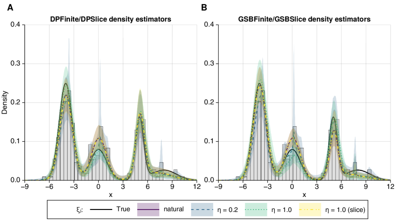
Figure 1: Histogram representation of the data with Monte Carlo density estimators and $95\%$ credible intervals for different choices $\xi_{j}$ and $\eta$ superimposed. Panel A shows the density estimators obtained from the DPFinite and DPSlice models. Panel B: shows the density estimators obtained from the GSBFinite and GSBSlice models.

Figure 1 shows the MC density estimators and $95\%$ credible intervals (CI) based on the $80,\!000$ samples taken from the posterior draws of each model, superimposed on the histogram of the data. Figure 1(A) shows the density estimators obtained from the DPFinite and DPSlice models while Figure 1(B) shows the density estimators obtained from the GSBFinite and GSBSlice models. In Figure 2 we show the ergodic means for the number of occupied clusters over iterations for all the models under the different choices of $\xi_{j}$ and $\eta.$

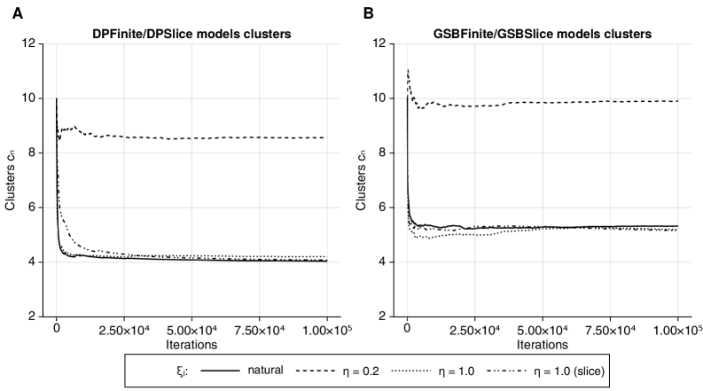
Figure 2: Ergodic means for the number of occupied clusters $c_{n}$ over iterations. Panel A shows the running average for DPFinite and DPSlice models for different choices of $\xi_{j}$ and $\eta.$ Panel B shows the running average for the GSBFinite and GSBSlice models.

We note how a small value of $\eta(=0.2)$ leads to a higher number of occupied clusters $c_{n}$ in the posterior for both DP/GSBFinite models (black dashed lines). This is reflected in the credible intervals of the density estimators in Figure 1 as shown from light-blue sharp peaks in Figure 1(A-B). For the other values of $\eta$ and the natural random sequence $\xi_{j},$ the DPFinite and DPSlice models quickly converge to the order of the data-generating mixture. The GSBFinite and GSBSlice models tend to yield slightly larger values of $c_{n}$, consistent with the over-clustering behavior reported in DeBlasi2020; Hatjispyros2023.

Table 1 reports the execution times (in seconds) of the compared algorithms. The Table suggests that the DPFinite model has faster execution times and scales better on larger data sets in particular when $\xi_{j}$ is chosen to be the natural random decreasing sequence. In order to show how the algorithms scale relatively to the sample size $n,$ we also report the execution times when the models have been applied on a sample of size $n=1000$ generated from Equation 17.

Table 1: Execution times (in seconds) for $100,\!000$ iterations of the algorithms for the four–component mixture of normals for different sample sizes.

	DP based models		GSB based models
$\xi_{j}$	$n=250$	$n=1000$	$n=250$	$n=1000$
natural	10.508	37.697	18.429	74.997
$\eta=0.2$	33.976	82.733	35.564	79.480
$\eta=1.0$	11.058	26.635	11.192	26.868
$\eta=1.0$ (slice)	20.242	64.697	21.492	71.570

• Note: Density estimator is evaluated on a grid of $500$ points. Less/more points in the grid results to faster/slower execution times.

5.2 Galaxy data

We now consider a well–known real data set in the mixture modeling literature: the galaxy data, consisting of the velocities (in $km/s$) of 82 galaxies from the Corona Borealis region. This data set has been widely used as a benchmark for mixture modeling, and several studies have suggested that the underlying distribution exhibits multimodality, with a consensus around three to six clusters (RichardsonGreen1997; RoederWasserman1997).

Our goal is to assess the flexibility of each method in capturing the observed multimodality and in identifying the effective number of components, namely the posterior behavior of the occupied-cluster count $c_{n}$.

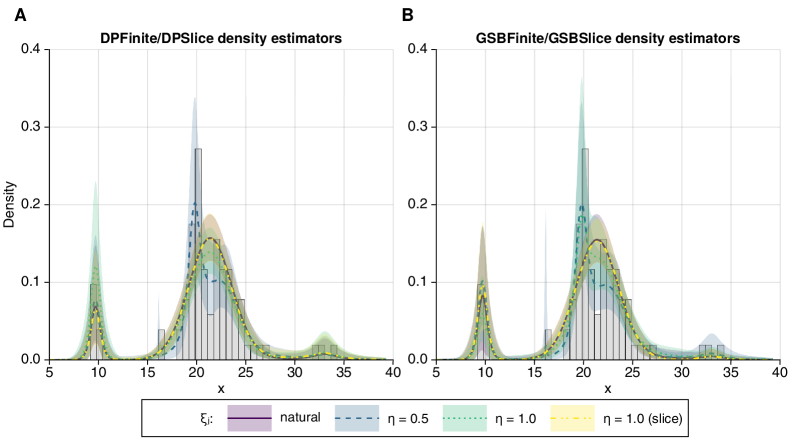
Figure 3: Monte Carlo density estimators obtained from the DPFinite and DPSlice models superimposed on the histogram of the galaxy data (Panel A), and the GSBFinite and GSBSlice models (Panel B).

As shown in Figure 3, all methods capture the multimodal structure of the data reasonably well. Each sampler produces a smooth fit that concentrates mass on a few modes, aligning with previous scientific assessments.

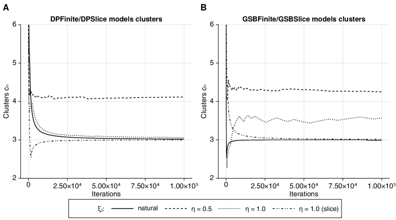
Figure 4: Ergodic means for the number of occupied clusters $c_{n}$ over iterations. Panel A shows the running average for DPFinite and DPSlice models for the different choices of $\xi_{j}$ and $\eta.$ Panel B shows the running average for the GSBFinite and GSBSlice models.

Figure 4(A) shows that the DPFinite and DPSlice models stabilize around three clusters, supporting the hypothesis of a small but nontrivial number of components. We note that imposing a small value of $\eta=0.5$ leads to a slightly overestimated value of $c_{n}$ (Figure 4 black dashed line).

In Table 2 we report the execution times (in seconds) for all the models in the comparison.

Table 2: Execution times (in seconds) for $100,\!000$ iterations of the algorithms for the galaxy data.

$\xi_{j}$	DPFinite/DPSlice	GSBFinite/GSBSlice
natural	5.269	5.827
$\eta=0.5$	14.449	9.434
$\eta=1.0$	7.056	6.428
$\eta=1.0$ (slice)	7.061	6.068

• Note: Density estimator is evaluated on a grid of $500$ points. Less/more points in the grid results to faster/slower execution times.

6 Conclusions

This paper develops a new perspective on Bayesian nonparametric mixture modeling by introducing an exact finite representation of species sampling processes. The key insight is that any mixture induced by a proper SSP within an SSM can be reparametrized via a finite mixture with a random $K$. This representation is not an approximation but a structural reformulation, in which the truncation level emerges as a latent variable with an explicit conditional distribution. In doing so, we preserve the full generality of infinite–dimensional SSP priors while gaining a tractable framework for inference.

Building on this representation, we proposed a Gibbs sampling algorithm that avoids the ad hoc algorithmic truncations required by generic slice methods. The resulting procedure is simple to implement, theoretically grounded, and applicable to a wide range of SSP priors used in mixture models, including Dirichlet, Pitman–Yor, geometric and more general stick–breaking families, as well as dependent–length constructions such as DSBw.

Our empirical results demonstrate the practical benefits of this approach. Across simulated mixtures and the benchmark galaxy dataset, the proposed finite–representation samplers successfully recover both the underlying density and a sensible posterior distribution for the effective number of occupied clusters $c_{n}$. Compared with alternative methods, they tend to converge more rapidly and avoid the systematic overestimation of clusters often observed in decreasing–weight models. In the simulation studies of Section 5, we therefore interpret the posterior of $c_{n}$ as a summary of the induced random partition, and compare it to the finite-mixture order of the data-generating model only as a diagnostic, not as a consistency claim for any underlying “true” number of components.

An important conceptual distinction emerging from our framework is between: (i) the finite–representation truncation level $K$; (ii) the random number of occupied clusters $c_{n}$ in a sample of size $n$; and (iii) the (fixed or random) number of components $m$ in classical finite mixture models, i.e. (4). In our construction, $K$ is a prior–level latent variable used to represent the SSP $G$ as an exact finite mixture; $c_{n}$ is a data–dependent random quantity measuring how many atoms are occupied in a given sample; and $m$ in finite mixture modeling is a structural parameter specifying a true finite number of components. These objects live at different levels of the hierarchy and are not directly comparable. In particular, it is generally inappropriate to interpret $c_{n}$ as an estimator of $K$, or $K$ as a “true” number of clusters.

While the relation between $m$ and $c_{n}$ is unknown in general for SSPs, it has been characterized in important special cases. For Gibbs–type priors with negative discount parameter $\sigma<0$ (GnedinPitman2006; LijoiMenaPrunster2007Biometrika; Lijoi2007; DeBlasi2013), the induced random probability measures can be written as mixtures of symmetric Dirichlet distributions with a prior on the number of blocks. In this finite–species setting, one can derive explicit conditional laws $\mathbb{P}(c_{n}=c\mid m=m^{\star})$ and $\mathbb{P}(m=m^{\star}\mid c_{n}=c)$ and show asymptotic concordance between posterior probabilities for $m$ and $c_{n}$ as $n\to\infty$; this is often presented under the label of “mixtures of finite mixtures” and gives a clear interpretation of $m$ as a genuine parameter (miller2018consistent). At the same time, part of the subsequent literature has used these results to suggest an “inconsistency” of $c_{n}$ as an estimator of $m$, or more broadly to argue against BNP methods based on SSPs. Our view is that this criticism is largely misplaced: the issue is one of identifiability of $m$ under a given model, not a generic inferential failure of nonparametric priors, and arises only when one insists on treating $c_{n}$ as if it were targeting a finite–mixture parameter $m$.

This discussion also clarifies the relationship between our finite representation and the so called mixtures of finite mixtures. In those models, the number of components $m$ (e.g., the number of blocks in a symmetric Dirichlet mixture) carries its own prior and is a genuine parameter; the law of the random measure depends on that prior, and under suitable conditions the posterior can be consistent for a finite “true” $m$ (DeBlasi2013; deblasi2015). In our finite representation, by contrast, $K$ is not a free modeling choice but a derived latent variable determined by the SSP weights and a decreasing sequence, and marginalizing over $K$ recovers exactly the original SSP prior. Thus the two constructions share a superficial form (finite mixture with random $K$) but encode fundamentally different modeling choices: mixtures of finite mixtures correspond to finite–species Gibbs–type priors with $\sigma<0$ and an explicit prior on the number of components, whereas our construction reparametrizes a fully nonparametric SSP without changing its support or its induced partition structure.

Overall, the framework presented here strengthens the connection between random partitions and mixture modeling, offering a unified and tractable view of SSP–based SSMs. We anticipate that this perspective will facilitate new developments in Bayesian nonparametrics, particularly in extending inference to more complex hierarchical and non–exchangeable structures, where finite representations may offer both conceptual clarity and computational advantages.